e ( u ' p ')x p 'x u ' 2 p 'x 2 u ' p 'x u ' u ' u u ' ' u ' 10 10 u ' u ' u ' u u ' u ' u ' u = u ' + p ' − u ' = − 2 u ' = = (2 u ' − ) 2( = 2( ) ) + 2 u ' :( ) + u = − 2 u u − x x x x x x x x x x t x x x € €   u ' ' 2 p ' € € + 2 u g + 2 f u u − u '

6 Turbulent Kinetic Energy and Dynamical Stability 6.1 TKE-Equation

In the foregoing chapter an equation has been derived for the (summed) velocity variances that is repeated here for convenience in its flux form

€

∂u'

∂t + u

∂u'

∂x

= − 2u

u

∂u

∂x

− ∂u

u'

∂x

+ 2δ

u

θ' θ



  

  g + 2f

ε

u

u

− 2

ρ u'

∂p'

∂x

+ 2νu'

∂

u'

∂x

^(5.34)

The last three terms on the rhs of (5.34) can be simplified as follows. Inserting the definition of

€

ε_ij3

(see definition in the note to Table 5.1) readily shows that the Coriolis term vanishes.

For the pressure term we note that

€

∂(u'

p')

∂ x

= u'

∂p'

∂ x

+ p' ∂u'

∂ x

^{, (6.1)}

of which the last term on the rhs vanishes due to the summation (continuity equation). In flux form the second last term on the rhs of (5.34) therefore reads

€

− 2 ρ ^u'

∂ p'

∂ x

= − 2 ρ

∂ u'

p'

∂ x

. (6.2)

For the last term on the rhs of (5.34) we note that

€

∂

u'

∂x

= ∂

∂x

(2 u'

∂u'

∂x

) = 2( ∂u'

∂x

)

+ 2u'

∂

u'

∂x

^{. (6.3)}

Therefore

€

2νu'

∂

u'

∂x

= ν ∂

u'

∂x

− 2ν ( ∂ u'

∂x

)

, (6.4)

The first term on the rhs of (6.4) is on the order of

€

10

while the second term is O (

€

10

). The rate of dissipation of TKE is therefore defined as

ε = : ν ( ∂u'

∂ x

)

, (6.5)

Recalling the definition of TKE (eq. 3.25), and with the above simplifications

(5.34) yields a conservation equation for TKE per unit mass, e :

- 2 -

€

∂ e

∂ t + u

∂ e

∂ x

= − u'

u'

∂ u

∂ x

− ∂ u'

e

∂ x

+ δ

u'

θ ' g θ − 1

ρ

∂ u'

p'

∂ x

− ε ^(6.6) The terms on the lhs (of (6.6) are the local temporal change and the advection term respectively. On the rhs we have the shear production, the turbulent transport of TKE, the buoyancy term, the pressure correlation term and the dissipation rate of TKE.

Clearly, TKE is strongly dependent on the stability of the flow through the buoyancy term. Under convective (daytime) conditions the turbulent heat flux is positive

€

u'

θ ^' > 0 and thus the buoyancy term is a production term. In contrary, under stable conditions (night time) this term becomes a sink and acts to damp TKE. Therefore, even under horizontally homogeneous conditions TKE exhibits a strong daily cycle (Fig. 6.1) and the local temporal change of TKE vanishes only during carefully selected periods of time.

Shear production of TKE

The first term on the rhs of (6.6) is always positive and thus a production term.

This can easily be seen by recalling that – for example in the vertical direction – the shear stress is directed towards the surface (

€

u'

u'

< 0) and is the result of friction, which a the same time leads to a positive gradient of the mean wind speed (

€

∂ u

∂ x

> 0 ). Or in more general terms, in a Newtonian fluid the shear stress can be expressed as proportional to the rate of deformation.

Therefore, all the individual products making up this term are negative and with minus sign we have a production term. Clearly, at least close to the surface the vertical shear stress makes up the dominant contribution to this term.

The shear production term describes the interaction of the turbulence with the mean flow. If the TKE equation has the form

€

∂ e

∂ ^{t + ... = − u'}

^u'

∂ u

∂ ^x

^{+ ... (6.7)}

the corresponding conservation equation for the mean kinetic energy (

€

E = 0.5 u

) reads

€

∂ ^E

∂ ^{t + ... = + u'}

^u'

∂ ^u

∂ ^x

^{+ ... , (6.8)}

thus showing that the shear production of TKE goes at the expense of mean kinetic energy of the flow.

Turbulent transport of TKE

First of all we note that – similar as with the second moments in the conservation equation for the mean variables – it is the flux divergence that enters the TKE equation. Assuming horizontally homogeneous conditions for the moment we further note that

€

∂ ^u'

e ∂ ^x

= ∂ ^(u'

u'

+ u'

u'

+ u'

∂ ^x

. Under

stable/neutral conditions the third order moments and especially the

skewness of the vertical velocity component are rather insignificant due to the

near-normal distribution of the velocity fluctuations and correspondingly small

is the turbulent transport term. In convective conditions, however, the non-

local mixing through large eddies changes the situation. Figure 4.8 shows the

profile of the skewness of the vertical velocity component under typical

convective stratification. Figure 1.8 has already paved the terrain for the

apprehension of large eddies being responsible relatively strong updrafts

(thermals) over a limited area and weaker compensating subsidence, thus

leading to a skewed distribution of the vertical velocity component.

- 4 -

Figure 6.1 Time variation of TKE as measured at three different levels on tower (lines) and from a low flying light research aircraft (circled symbols).

The numbers in the abscissa indicate the day-of-year in 1999 (from Weigel and Rotach 2004).

From Fig. 4.8 we see that close to the surface (essentially in the lower third or so of the CBL)

€

− ∂ ^u'

∂ ^x

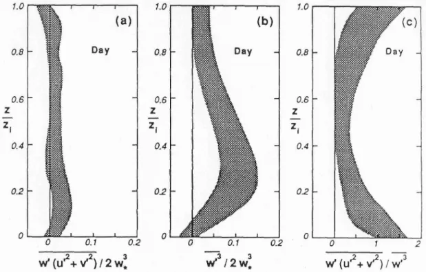
< 0 and hence turbulent transport of TKE constitutes a loss term. This is clear since the dominant (shear) production occurs close to the surface and through the transport term the upper parts of the boundary layer gain TKE. Figure 6.2 shows that also horizontal velocity variance is transported in a similar fashion away from the surface – and also from the top of the CBL downwards - through the transport term.

Figure 6.2 Vertical profiles of the mixed third moments in CBL’s (shaded ranges). From Stull (1988).

The pressure correlation term is the least known of all contributions to the TKE budget, mainly due to observational problems. It is generally considered to be small and therefore often treated as a residual term in TKE budget studies.

Dissipation of TKE

The rate of dissipation of TKE is due to its definition (eq. 6.5) and meaning

always negative. Close to the surface it is naturally at maximum (Fig. 6.3) due

to the dominant shear production there. The dissipation of TKE eventually

leads to kinetic energy of the flow being transformed into heat. Even close to

the surface, where it is at maximum, this heat input is negligibly small as

compared to all the other terms in the energy budget equation and therefore usually (and safely) neglected.

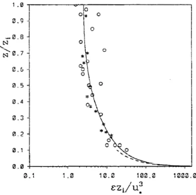
Figure 6.3 The near neutral profile for the dissipation rate of TKE, solid line, compared with measurements. Data: * Grant (1992), o Brost et al (1982). The dashed line represents a surface layer parameterization after Vogel and Frenzen (1992). From Rotach et al (1996).

Idealised profiles

Under ideally neutral, horizontal homogeneous and steady state conditions

the shear production of TKE is balanced by dissipation (Fig. 6.4). Clearly,

such conditions are difficult to meet in real flows and often other processes

contribute to the TKE budget. The four dominating terms in near steady-state

daytime ABL’s are summarised in Fig. 6.5. Again it can be seen that close to

the surface shear production and dissipation dominate and an important

source of TKE in the central part of the boundary layer is turbulent transport

away from the surface. The buoyancy term essentially follows the profile of

the turbulent heat flux with a maximum at the surface and a minimum (loss of

TKE due to the entrainment process) at the top. After sunset the buoyancy

term also becomes a sink (Fig. 6.6, left panel) and shear production is way

too weak to maintain the TKE levels of the day. Therefore, after some hours

TKE levels are largely reduced and so are the budget terms (Fig. 6.6, right

panel).

- 6 -

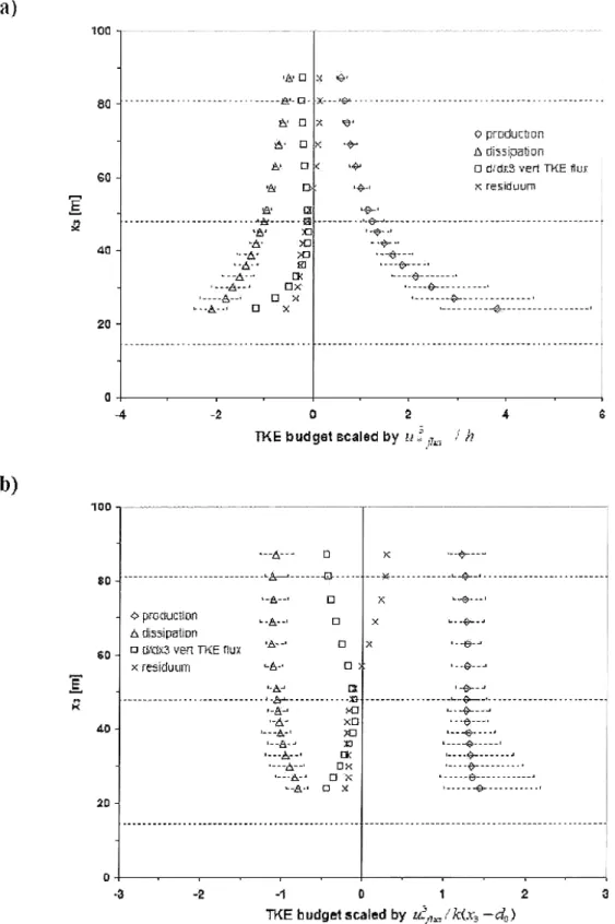
Figure 6.4 Profiles of budget terms in the TKE equation over an urban surface in a

wind tunnel. The dashed lines indicate (from the bottom upwards) the

mean building height, the height of the roughness sublayer (section

8.2) and the height of the inertial sublayer. From Feddersen (2005).

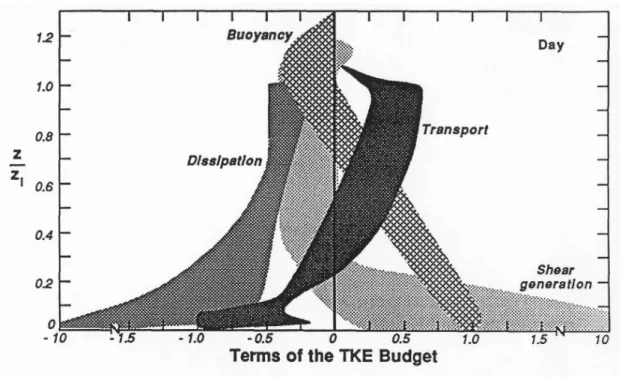
Figure 6.5 Vertical profiles of budget terms in the TKE equation under convective conditions (shaded areas give spread). From Stull (1988).

Figure 6.6 Modelled budget terms of the TKE equation during ‘night 33-34’ in

the Wangara experiment. Left panel at 6pm (day 33) and right panel

at 2 am (day 34). From Stull (1988).

- 8 -

6.2 Stability Measures

Until now we have used stability as a discriminating criterion for different types of boundary layer states. In this we have always silently assumed that with

‘stability’ the static stability, i.e. the gradient of the potential temperature was referred to. However, the stability of a turbulent flow not only depends on the thermal stratification but also on the shear production of TKE, which is even dominating in various regions of the ABL. In loos terms we may say that a turbulent flow is very unstable if shear production is supported by additional buoyancy production, is near-neutral if the buoyancy term is small and finally is stable if buoyancy acts to damp TKE. It seems therefore appropriate to define a dynamical stability measure, which takes into account not only the sign of the buoyancy production/damping term but also the strength of the shear production.

6.2.1 The Flux Richardson number

One of the pioneer’s of atmospheric turbulence research, L.F. Richardson, has been the first to introduce a stability measure based on the TKE budget equation (6.6). His simplifying (idealising) assumptions were to consider a quasi-stationary (

€

∂ / ∂t = 0 ), horizontally homogeneous (

€

∂ / ∂x

= ∂ / ∂x

= 0 ) flow without subsidence (

€

u

= 0 ) and a coordinate system aligned with the mean wind (

€

u

= 0 ). With this eq. (6.6) becomes

€

0 = − u'

u'

∂ u

∂ x

− ∂ u'

e

∂ x

+ u'

θ ' g θ ⁻

2 ρ

∂ u'

p'

∂ x

− ε . (6.9)

Based on the this idealized TKE budget equation Richardson identified the shear production and the buoyancy terms as the dominating terms, based on which he defined a dynamical stability measure that is since then known as the Flux Richardson Number,

€

R

:

€

R

= : g θ

u'

θ' u'

u'

∂u

∂x

. (6.10)

Even if the assumption of neglecting especially the dissipation term may not prove particularly good (cf. Fig. 5.4)

€

R

has become an essential variable in defining the turbulence state of atmospheric flows. Its most obvious property is that

€

R

< 0 for unstable conditions,

€

R

= 0 for neutral flows and

€

R

> 0 in stable conditions. If both shear production and buoyancy contribute to TKE production there is no theoretical limitation to

€

R

(at least not in the idealised assumption of its derivation) although it is hardly observed to become smaller than –10. On the stable side we readily observe that production of TKE is larger than damping if

€

R

< +1 . For larger Richardson numbers, no turbulence

can be maintained even if shear production should exist, simply because it is readily damped away by the stratification. For

€

0 < R

< 1 the flow is statically stable (

€

∂θ / ∂ x

> 0 ) and dynamically unstable in the sense that turbulence can

exist. Still, this consideration has neglected the dissipation of TKE, which

certainly (and substantially) will contribute to the suppression of turbulence.

Equating the total production (still only shear production) with the ‘total’

suppression (buoyancy plus dissipation terms) yields an expression for a

‘critical’ state, in which turbulence can ‘just’ be maintained:

€

g

θ u'

θ ' − ε u'

u'

∂u

∂x

= 1 . (6.11)

Equation (6.11) can be expressed in terms of

€

R

to yield a ‘critical’

Richardson number above which damping of TKE is dominating over production

€

R

= 1 + ε u'

u'

∂ u

∂ x

. (6.12)

The sign of the second term on the rhs of (6.12) is always negative thus indicating that somewhere between

€

0 < R

< 1 this critical state is reached (see below, 6.2.2). Beyond this point, turbulence occurs only sporadically, i.e.

it may be produced locally and is ‘dissipated away’ quite quickly. In terms of scaling regimes (Fig. 4.4) this state of the stable boundary layer is referred to as intermittency.

6.2.2 The Gradient Richardson number

The diagnostics of the dynamic stability using the Flux Richardson number requires the knowledge of the turbulent fluxes (eq. 6.10), which are often not available (e.g., in a numerical model with a first order turbulence closure).

Also, as a measure for the transition between laminar and turbulent states of a flow, a measure might be desirable that is non-zero in both

. Therefore as an approximation, K-Theory (Section 5.2.1) is used to define the so-called Gradient Richardson Number,

€

Ri . Thereby the simplifying assumption is made that the exchange coefficients for momentum,

€

K

, and for sensible heat

€

K

are equal, thus

€

Ri =: g θ

∂θ ∂x

( ∂ u

∂ x

)

. (6.13)

Clearly,

€

Ri is easier to determine than

€

R

but it still has the ‘theoretical‘

foundation of employing in an idealised fashion the TKE budget equation for

its definition. It has the same properties in terms of sign as the Flux

Richardson number (positive for statically stable and negative for statically

- 10 -

unstable conditions). The flux and Gradient Richardson numbers are related through

€

R

= Ri K

K

^{. (6.14)}

In the literature a critical Richardson number (cf. 6.12) is always given in terms of

€

Ri rather than

€

R

. Observational evidence and some further theoretical considerations (Nieuwstadt, 1984) indicate that

€

Ri

≈ 0.25 , (6.15)

i.e. at a value substantially smaller than one the action of buoyancy and dissipation make it impossible to maintain a fully turbulent state.

6.2.3 The Bulk Richardson number

If the evaluation of gradients is still beyond the possibilities an even simpler approach to dynamic stability is the Bulk Richardson Number,

€

Ri

. In this further simplification the gradients are replaced by differences, and hence

€

Ri

= : g θ

Δ θ Δx

(Δu

)

. (6.16)

The Bulk Richardson number is often used as an approximation for the entire boundary layer and hence the differences are taken between the ABL top and the surface (in this case

€

Δ u

reduces to

€

u

because the mean speed vanishes at the surface). Clearly

€

Ri

has the advantage of simplicity but the linearization implied in the transition between

€

Ri and

€

Ri

is not generally based on solid ground.

6.2.4 Stability measure in the Surface Layer In Chapter 4 the non-dimensional quantity

€

z / L , where

€

L is the Obukhov length, has been found to be the ‘one and only’ dimensionless group to describe turbulence variables in the Surface Layer. This result was achieved using similarity theory. We may use this result to expressing the simplified TKE budget (6.9) in terms of SL variables and in non-dimensional form. For this we multiply each term by

€

kx

/ u

and replace the turbulent fluxes by their surface values (

€

−u'

u'

→ −(u'

u'

)

= u

and

€

−u'

θ ' → −(u'

θ ')

:

€

0 = kx

u

∂u

∂x

− kx

u

∂u'

e

∂x

− kx

g(u'

θ')

θ u

− 2kx

ρ u

∂u'

p'

∂x

− kx

u

ε = Φ

− Φ

+ z

L − Φ

− Φ

. (6.17)

The chosen scaling exactly

corresponds to Richardson’s approach in that the former buoyancy term now corresponds to

€

z / L and expresses the ratio between buoyancy production/damping and shear production of TKE.

2 With the additional von Kàrmàn constant and the constraint of surface fluxes.

Monin-Obukhov similarity theory then predicts that all the ‘Phi functions’ in (6.17) be a function of

€

z / L alone – what has been shown to be a good prediction for, e.g.

€

Φ

(Fig. 4.3) and a useful approximation for

€

Φ

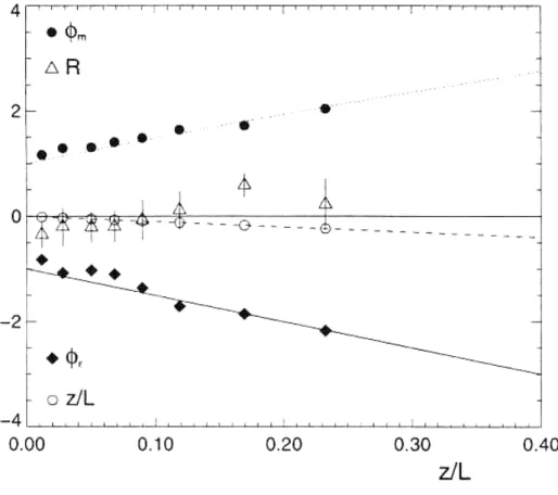
even outside the SL (Fig. 6.3) under near-neutral stratification. Figure 6.7 shows the dominating terms (with the transport and pressure terms as residual) over a horizontally homogeneous snow surface on the Greenland ice sheet.

Neglecting the turbulent transport and pressure correlation terms for a moment we find from this analysis that the sum ‘shear production minus dissipation’ in its non-dimensional form is linearly related to

€

z / L , an observation that is often confirmed to approximately hold in the SL.

Fig. 6.7 Terms of the non-dimensional TKE budget equation in the SL over a horizontally homogeneous snow-covered surface on the Greenland ice sheet. The dotted line corresponds to (4.24), the solid line is a parameterization (stable stratification) for the non-dimensional dissipation rate, the dashed line is the 1:1 line for the buoyancy term.

The triangles denote the residuum term. Symbols as bins over stability ranges. From Forrer (1999).

Finally, using the non-dimensional wind shear (eq. 4.14) and the non-

dimensional temperature gradient (eq. 4.25) we can find a relation between

- 12 -

€

Ri = z L

Φ

Φ

. (6.18)

And with (6.14) we obtain

€

R

= K

K

Ri = x

L

Φ

( Φ

)

K

K

. (6.19)

These equations can be used if, e.g. gradients of wind speed and temperature are available from which

€

z L is derived iteratively.

References Chapter 6

Brost, R. A., Wyngaard, J. C. and Lenschow, D. H.: 1982, Marine stratocumulus layers. Part II: Turbulence budgets J. Atmos. Sci, 39, 818-836

Forrer, J.: 1999, The structure and turbulence characteristics of the stable boundary layer over the Greenland ice sheet, ETH dissertation 12803, 137pp.

Grant, A. L. M.: 1992, The structure of turbulence in the near-neutral atmospheric boundary layer, J. Atmos. Sci, 49, 226-239

Nieuwstadt, F.: 1984, The Turbulence Structure of the Stable Nocturnal Boundary Layer, J.

Atmos. Sci., 41, 2202–2216.

Rotach M.W., Gryning, S.-E. and Tassone C.: 1996, A Two-Dimensional Stochastic Lagrangian Dispersion Model for Daytime Conditions, Quart. J. Roy. Meteorol. Soc., 122, 367-389.

Stull RB: 1988, An introduction to Boundary Layer Meteorology, Kluwer, Dordrecht, 666pp.

Vogel, C. A. and Frenzen, P.: 1992, A new study of the TKE budget in the surface layer.

Proceedings 11^th Symposium on Turbulence and Diffusion, Portland, Sept. 29-Oct. 2 (1992), 161-164.

Weigel AP and Rotach MW (2004): Flow structure and turbulence characteristics of the daytime atmosphere in a steep and narrow Alpine valley, Q J R Meteorol Soc, 130, 2605–2627.