Originally published as:
Qu, Y., Wu, N., Guse, B., Makarevičiūtė, K., Sun, X., Fohrer, N. (2019): Riverine phytoplankton functional groups response to multiple stressors variously depending on hydrological periods. - Ecological Indicators, 101, pp. 41—49.
DOI: http://doi.org/10.1016/j.ecolind.2018.12.049
1 1
2
Riverine phytoplankton functional groups response to multiple
3
stressors variously depending on hydrological periods
4 5
Yueming Qu1*, Naicheng Wu 1,2,3*, Björn Guse1,4,Kristė Makarevičiūtė5, Xiuming Sun1, Nicola
6
Fohrer1
7
1 Department of Hydrology and Water Resources Management, Institute for Natural Resource
8
Conservation, Kiel University, Olshausenstr. 75, 24118 Kiel, Germany
9
2 Aarhus Institute of Advanced Studies, Aarhus University, Høegh-Guldbergs Gade 6B, 8000 Aarhus
10
C, Denmark
11
3 Department of Bioscience, Aarhus University, Ole Worms Allé 1, 8000 Aarhus C, Denmark
12
4 GFZ German Research Centre for Geosciences, Section 5.4 Hydrology, Potsdam, Germany
13
5 GEOMAR Helmholtz Centre for Ocean Research Kiel, DüsternbrookerWeg 20, 24105 Kiel,
14
Germany
15
* Corresponding authors: yqu@hydrology.uni-kiel.de (Y. Qu), nwu@hydrology.uni-kiel.de (N. Wu)
16 17
2
ABSTRACT
18
Rivers and related freshwater ecosystems are facing increasing natural disturbance and
19
anthropogenic stressors. Understanding the key ecological processes that govern the riverine biota in
20
aquatic ecosystems under multiple pressures has crucial importance. However, there is still
21
insufficient knowledge in quantifying of stressors interactions. Moreover, the understanding of the
22
responses of riverine phytoplankton to multiple stressors is still scarce from catchment aspect. As an
23
interdisciplinary study, the catchment hydrological processes were linked to ecological responses in
24
this study, and we chose phytoplankton functional groups (PFGs) instead of taxonomic
25
classifications of algae to examine their responses to land-use pattern (L), hydrological regime (H),
26
and physicochemical condition (P) across two contrasting hydrological periods (dry, wet). The
27
traits-based phytoplankton functional groups are highly suggested as robust bio-indicators for better
28
understanding the current ecological status. The hydrological regime was described by a matrix
29
indices of hydrological alteration based on the outputs of a well-established ecohydrological model
30
(SWAT). The results from variation partitioning analysis showed that P and H dominate during the
31
dry period and P in high flows. Structural equation models (SEM) showed that the skewness of 7
32
days discharge emerged as a key driver of H, and had always an indirect effect on functional group
33
TB (benthic diatoms) during both hydrological periods. The functional group M (mainly composed
34
by Microcystis) has directly related to phosphorous in both periods, while indirectly to L of urban
35
area in high flow period, and water bodies in low flow period. This study emphasized that climate
36
change and anthropogenic activities such as altering flow regime and land-use pattern affect directly
37
or indirectly riverine phytoplankton via physicochemical conditions. In addition, our findings
38
3
highlighted that biomonitoring activities require detailed investigation in different hydrological
39
periods. SEM is recommended for improved understanding of phytoplankton responses to the
40
changing environment, and for future studies to fulfill the increasing demand for sustainable
41
watershed management regarding aquatic biota.
42
Keywords:
43
Phytoplankton functional groups,
44
Land-use pattern,
45
Hydrological regime,
46
Physicochemical condition,
47
Structural equation model
48 49
4
1. Introduction
50
Riverine phytoplankton is one of the vital primary producers in the river ecosystem, and acts as
51
robust bio-indicator responding to multiple stressors (Hilton et al., 2006). It is widely used for
52
bio-assessment of freshwater ecosystems in recent years (EC, 2000). Benthic diatoms are one of
53
significant elements of riverine phytoplankton recruitment, especially in the fine substrate rivers
54
(Bolgovics et al., 2017). Short water residence time lead to benthic diatoms dominance (Reynolds,
55
1994; Wang et al., 2018), while dynamic flow velocity results in shifts of the share of benthic
56
diatoms in the phytoplankton community (Wu et al., 2007). Moreover, flow alteration influence
57
riverine phytoplankton assemblages by altering nutrient delivery, light availability, dewatering of
58
habitats or severe vertical mixing (Reynolds, 2006). Despite diatom dominance, several studies
59
demonstrate that running water can also suffer the negative consequences of cyanobacterial blooms,
60
resulting from anthropogenic eutrophication and changing environment (Bowling et al., 2016;
61
Stanković et al., 2012). Intensive agriculture and urbanization strongly affect freshwater biodiversity
62
through flow modification and nutrient over-enrichment by fertilizer, pesticides, and sewage fluxes
63
(Bussi et al., 2016; Harris and Smith, 2016; Katsiapi et al., 2012). Changing climate conditions,
64
specifically global warming and altered rainfall patterns, play additional interactive roles in
65
modulating cyanobacterial blooms frequency, intensity and geographic distribution in a long-term
66
aspect (Paerl, 2017; Paerl et al., 2011). Therefore, multiple stressors including natural disturbances
67
(drought and floods) and anthropogenic stressors (human-induced water pollution, eutrophication)
68
are affecting riverine phytoplankton directly or indirectly. Understanding the key ecological
69
processes that govern riverine phytoplankton community in aquatic ecosystems under multiple
70
5
pressures has crucial importance. It is a fundamental prerequisite for robust bio-assessment, as well
71
as sustainable watershed management. However, investigations and analysis of stressors interactions
72
were much insufficient. Studies about the response of riverine phytoplankton to multiple stressors
73
from catchment scale are still scarce.
74
Interactions of multiple stressors determine the occurrence and survival of algae. In turn,
75
phytoplankton response to stressors by associated functions of tolerance, preference, and sensitivities
76
of distinct traits (Kruk et al., 2017; Litchman and Klausmeier, 2008). In this study, we chose
77
phytoplankton functional groups (PFGs) instead of taxonomic classifications of phytoplankton
78
dynamics to investigate their response to multiple stressors in a better way: land-use pattern (L),
79
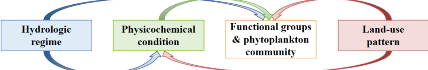
hydrological regime (H) and physicochemical condition (P) (see Fig. 1, a schematic diagram
80
developing a conceptual framework). PFGs concept suggested aggregating species with similar
81
features into a few functional groups. Each group was described according to the physiological,
82
morphological and ecological traits, as well as common environmental sensitivities and tolerances
83
(Borics et al., 2007; Reynolds et al., 2002). For elaboration of the phytoplankton-based quality
84
assessment, Borics et al. (2007) replenished and evaluated PFGs in rivers, considering four parts:
85
trophic state, turbulence character, time sufficient for development of the given assemblage and risk.
86
Code TB (composed by benthic diatoms) and code M (mainly composed by limnophilic Microcystis
87
spp.) represent two highly different functional groups of riverine phytoplankton. TB is assigned to
88
mesotrophic, highly lotic preference benthic species with low risk of harm, while M assigned to
89
hypertrophic nutrient status, lentic preference, climax assemblages with potential toxicity. Mischke
90
et al. (2011) also selected the proportions of Cyanobacteria and Pennales (as typical benthic diatom)
91
to assess the trophic status of German Rivers. They concluded an unhealthy status with a high
92
6
proportion of Cyanobacteria, while they detected a healthy status with a high percentage of Pennales.
93
We were working with a lentic-lotic continuum watershed in a rural area under natural hydrology
94
disturbance and human-induced stressors.Based on the previous investigation of this catchment, we
95
found nutrients, especially the nitrate loads, were highly related with agriculture activities in the
96
Treene basin (Haas et al., 2016). TB were dominant in most of the study area, while their share
97
varied in time and space(Qu et al., 2018b). The temporary intensive occurrence of Microcystis in dry
98
season received high concerns from the local stakeholders (Qu et al., 2018a). Therefore, we are
99
especially interested in these two functional groups TB and M, in addition to the phytoplankton
100
community characteristics. We hypothesized that: 1) High flow condition promote to TB domination
101
over the others; 2) High share of agriculture land-use rise ascendancy of M in the community. Our
102
study aims to disentangle the causal-effects relationship of multiple stressors and riverine
103
phytoplankton community (indicated by PFGs) from wet and dry seasons. The answers would give
104
novel insights into the complex pathways of joint impact of natural and anthropogenic descriptors on
105
riverine phytoplankton community in lowland rivers across contrasting hydrological periods.
106
107
Fig. 1 Schematic diagram showing the major factors (e.g., hydrological regime, physicochemical condition, and land-use 108
pattern), which govern the pattern of phytoplankton functional groups and community structures. Those controls include 109
state factors, interactive controls, direct controls and indirect controls, which eventually causes the difference of 110
phytoplankton communities.
111 112
2. Material and methods
113
7
2.1. Study area and sampling sites
114
This study was carried out in Treene River, a lowland watershed located in the northern
115
Germany. As a lowland catchment, the maximum elevation of Treene basin is 76 m, with watershed
116
area of 517 km2. The Treene catchment is in a temperate climate zone, which is influenced by marine
117
climate. Meanwhile it has a typical seasonal pattern of discharge, with the highest water flow in
118
winter and the lowest in summer and autumn (Guse et al., 2015a). Field surveys were carried out in
119
two hydrological periods (a wet period in December 2014 and a dry period in September 2015) on 59
120
sampling sites which covered mainstream and tributaries of the catchment. The abbreviation of the
121
site names are according to each sub-basin where they are located in: Bo for Bollingstedter Au, Je for
122
Jerrisbek, Ju for Juebek, Ki for Kielstau, Sa for Sankermark See, and Tr for the mainstream of
123
Treene. The numbers count along the longitudinal axis of rivers from the outlet to upstream. The
124
sampling points in close distance of lakes are not located in the lake, but rather are situated
125
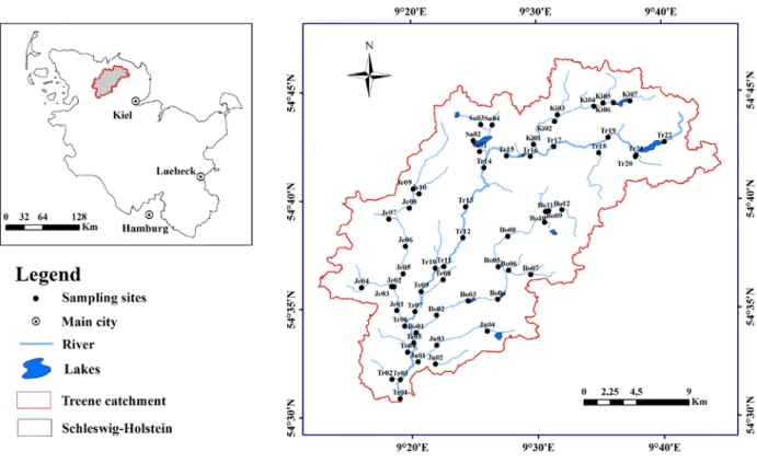
systematically downstream following the lakes (Fig. 2).
126
8 127
Fig. 2 The location of the Treene catchment and 59 sampling points in Schleswig-Holstein state of Germany.
128 129
2.2. Land-cover pattern analysis (L)
130
The catchment landscape is dominated by agricultural land-use. Around 50% of the area is
131
covered by arable land, and around 30% by winter pasture. Soils in the north of the catchment
132
(natural region of Angeln) are nutrient-rich and have a pH value ranging 6 to 7, while the pH of soils
133
in the south-east of the catchment (Geest) varies from 4 to 5.5 (Tavares, 2006). Therefore, in the
134
Angeln natural region, corresponding to Kielstau and Treene upstream catchments, agricultural fields
135
are more common, meanwhile, in the southern Geest region (e.g., Jerrisbek and Juebek catchments)
136
pastures constitute to a bigger part. The Treene catchment can be characterized by a slightly
137
undulating landscape, with various depressions and lakes (Kiesel et al., 2010). Land-use data was
138
provided by the Schleswig-Holstein State Bureau of Surveying and Geo-information
139
(LVERMGEO-SH, 2012). The land-use analysis performed via ArcGIS software (Version 10.0, ESRI,
140
9
US) processing (Fig. A. 1). Eight land-use types were classified: agricultural land-generic (AGRL),
141
forests (FRST), rangeland (RNGE), industrial area (UIDU), urban areas (URMD), water bodies
142
(WATR), wetland (WETL) and winter pasture (WPAS). The upstream watershed area from each
143
sampling site was accumulated, and the land-use within this area was considered as the land-use
144
pattern affecting the sampling site. In this case, the sites located at downstream and near to the lakes
145
or cities presented a higher percentage of water bodies or urban area. For example, the sites located
146
on the upstream region of a city has none percentage of urban area land-use, while the downstream
147
sites have decreasing percentages along the river flow.
148
2.3. Hydrological regime analysis (H)
149
Except for water depth and velocity which were measured in situ at the sampling points
150
(velocity – using FlowSens Single Axis Electromagnetic Flow Meter, Hydrometrie, Germany), the
151
hydrological regime was mainly described by the indicators of hydrological alteration (IHA) (Olden
152
and Poff, 2003). The IHA, illustrating the hydrographic signatures from the duration, frequency,
153
timing magnitude and rate of flow events, are ecological relevant and can be calculated based on
154
daily discharge data and are also used in hydrology (Kiesel et al., 2017; Pool et al., 2017). The daily
155
discharge time series in this study based on the output of the ecohydrological SWAT model (Soil and
156
Water Assessing Tool). In this model application, the model discretization for the Treene catchment
157
resulted into 108 sub-basins. In a multi-site calibration, six hydrological stations which distributed in
158
the catchment were used to consider the spatial heterogeneity in reproducing discharge. The
159
modeling period subdivided into a calibration (2001 to 2005) and a validation period (2006 to 2016).
160
To evaluate the model performance, we used three well-known performance measures:
161
Nash-Sutcliffe Efficiency, Percent Bias and RSR (root mean square error divided by standard
162
10
deviation) (see Guse et al., 2015b for details). Daily modeled discharge values were used for
163
subbasins in which at least one sampling point located. At this moment, the sampling points were
164
related to the model results from the closest outlet of a sub-basin outlet. We used 57 hydrological
165
indices from IHA describing the traits of hydrological regime. The final hydrological matrix included:
166
magnitude, frequency, rate of flow events and in situ measurement (Table A.1).
167
2.4. Physicochemical factors analysis (P)
168
Physicochemical factors collection included a field in situ measurements and laboratory
169
measurement. Water temperature (WT), pH, electric conductivity (EC) and dissolved oxygen (DO)
170
of the surface water were measured in situ using Portable Meter (WTM Multi 340i and WTW Cond
171
330i, Germany) at each sampling site. Simultaneously, two water samples were stored in pre-cleaned
172
plastic bottles (500 ml each) for nutrient analysis in the laboratory. They were partially filtered
173
through GF/F glass microfiber filter (Whatmann 1825-047) for collecting the total suspended
174
substances. Both filtered and unfiltered samples were kept frozen at -20 ℃ until measurement.
175
Concentrations of total phosphorus (TP), phosphate-phosphorus (PO43--P), ammonium-nitrogen
176
(NH4+-N), nitrate-nitrogen (NO3--N), nitrite-nitrogen (NO2--N), chloride (Cl-) and sulfate (SO42-)
177
were measured using the standard methods of DEV (Deutsche EinheitsverfahrenzurWasser-,
178
Abwasser- und Schlammuntersuchung). Dissolved inorganic nitrogen (DIN) was defined as the
179
summation of nitrite-nitrogen (NO2--N), nitrate-nitrogen (NO3--N) and ammonium-nitrogen
180
(NH4+-N), and the nitrogen to phosphorus ratio (NPR) is the ratio between DIN and TP. In this study,
181
we chose DIN:TP ratio instead of the TN:TP ratio, since DIN:TP can better discriminate the N and P
182
limitation of phytoplankton (Bergström, 2010). Total suspended solids (TSS) were measured
183
according to Standard Operating Procedure for Total Suspended Solid Analysis (Federation and
184
11
Association, 2005).
185
2.5. Phytoplankton collecting and processing
186
Phytoplankton samples were quantitatively analyzed with a known concentration from the
187
subsurface (5 - 40 cm) water of the river by plankton net. Identification included two steps. First, soft
188
algae was identified in a Fuchs-Rosenthal chamber with an optical microscope (Nikon Eclipse
189
E200-LED, Germany) at ×400 magnification, after employing the sedimentation method for the
190
samples (Sabater et al., 2008). Taxonomic identification was based on the references of Hu and Wei
191
(2006) and Burchardt (2014). Second, for further determination of the diatom species in the samples,
192
permanent slides were prepared after oxidization (using 5ml of 30% hydrogen peroxide, H2O2, and
193
0.5ml of 1mol/l hydrochloric acid, HCl), and then 0.1 ml of the diatom-ethanol mix was transferred
194
on a 24×24 mm coverslip. Diatoms were identified with the optical microscope (Nikon Eclipse
195
E200-LED, Germany) at ×1000 under oil immersion, based on the key books by Bey (2013),
196
Hofmann et al. (2011) and Bak et al. (2012). Algal biomass was calculated using the approximation
197
of cell morphology to regular geometric shapes, assuming the fresh weight unit as expressed in mass,
198
where 1 mm3/L = 1 mg/L (Huang, 2000; Wetzel and Likens, 2013). We then calculated the relative
199
biomass of every species as their abundance. Based on the criteria proposed by Reynold (2002),
200
species that contributed more than 5% of the total biomass were sorted into functional groups, and
201
the phytoplankton functional classification was done according to Reynolds et al. (2002), Borics et al.
202
(2007) and Padisák et al. (2009). Species not mentioned in the references were assigned to a group
203
according to their morphological and ecological characteristics and the environmental conditions
204
prevailing during their greatest occurrence (Devercelli, 2006). In this study, we specially focused on
205
the functional group M (species mainly from genus: Microcystis consisted by Microcystis
206
12
aeruginosa, M. wesenbergii, M. viridis) and TB (mainly composed of benthic Pennales, typically
207
genus such as: Navicula, Nitschia, Gomphonama, Fragilaria). From the references, this two group of
208
algae have different strategies, preference of living, and they present two characteristic conditions:
209
highly lotic river sections with TB dominance, while M dominance in eutrophicated lentic habitats
210
(Borics et al., 2007).
211
2.6. Statistical analysis
212
For achieving the best performance, the phytoplankton functional groups abundance matrix was
213
Hellinger transformed (Legendre and Gallagher, 2001; Legendre and Legendre, 2012). Firstly, the
214
analysis of PERMANOVA was conducted for testing the difference of PFG composition (function:
215
adonis of the R-package: vegan). In the meanwhile, the three sets of abiotic variables (i.e., L, H and
216
P) collinearity was tested when using all variables in the model of explaining variations of
217
phytoplankton communities (function: cor of the R-package: stats). Afterwards, a forward selection
218
(Blanchet et al., 2008) was carried out to choose a parsimonious subset of explanatory variables
219
(function: forward.sel of the R-package: adespatial), and then the multivariate community structure
220
was modeled under variation partitioning analysis (Borcard et al., 1992) (function: rda, varpart of
221
the R-package: vegan). We then constructed structural equation model (SEM) (Westland, 2016) for
222
quantitative evaluation of the relationship between human and natural stressors on PFG composition,
223
as well as the potential effect of land-use and hydrology on in-stream nutrients. We used
224
reduced-multidimensional data rather than original PFG matrices in the analysis since SEM can only
225
handle one-dimensional variables. Nonmetric multidimensional scaling (NMDS) ordination was
226
applied to produce reduced-dimensional data of PFG composition, measured as the first NMDS axis
227
scores for each site (i.e., NMDS1) to represent the main condition of the whole phytoplankton
228
13
community composition (function: metaMDS of the R-package: vegan). To achieve the SEM, we
229
first proposed the conceptual model for the three bio-indicators (PFG: TB, M and NMDS1). The
230
conceptual model included all possible pathways between the response variables and their key
231
abiotic variables, which identified by general linear model (function: glm and step of the R-package:
232
stats). In addition to the direct pathways, we also checked the indirect ones to see if variables exerted
233
further effects via mediation variables. From the initial model, we then specified the pathways. All
234
non-significant paths were eliminated stepwise until all remaining paths were significant related to
235
the response variables. Standardized path coefficients were calculated for each pathway for a better
236
comparable in the SEM. The overall final model fit was evaluated with root mean square error of
237
approximation (RMSEA), and the comparative fit index (CFI). RMSEA approach to 0, and CFI close
238
to 1.0 indicate a good fit of the model (Grace, 2006). In this study, SEM was constructed by sem in
239
the R-package: lavaan.
240
All analyses were conducted with the R software (version 3.5.1, R Development Core Team,
241
2018).
242
3. Results
243
3.1. Description of watershed hydrological regime and physicochemical condition
244
From the model outputs, the indicators of hydrological alteration varied across the two studied
245
periods. Water flow has a higher magnitude and fluctuation in the high flow (December) than in the
246
low flow period (September) (e.g., at the outlet of the catchment Tr01, Fig. A. 2). Some other typical
247
hydrological indices, for instance, H20 which represents the skewness of seven days of discharge,
248
has an opposite spatial trend during these two periods (Fig. A. 3). The index H20 ranges from -0.775
249
14
to 2.439. Most values of H20 were positive with a range of 0.043 to 2.439. They were negative
250
skewed only in the upstream of the main river (specifically sites: Tr16 - Tr22) in high flow period,
251
and tributary Jerrisbek during dry season. We observed a relatively high value in the tributary
252
Jerrisbek during the wet season (with an average value of 2.038). The key hydrological indicators
253
were summarized after pre-selection excluding the ones with significant multi-collinearity (Table 1).
254
The local physicochemical variables measured in situ varied considerably among different
255
hydrological periods and sub-catchments (Fig. A. 4). Firstly, the difference of water temperature
256
(WT) in two seasons was remarkable, and mean values in December 2014 and September 2015 were
257
5.69 ℃ and 14.24 ℃, respectively (Table 1). The value of pH followed a similar pattern in different
258
sub-basins, while mean value in September was slightly higher than in December (8.084 > 7.487,
259
Table 1). The concentrations of ammonium-nitrogen (NH4+-N) showed a higher concentration in
260
December compared to September (average: 0.307 mg/L > 0.158 mg/L, Table 1, also see more
261
details in Fig. A. 4). Conversely, nitrate-nitrogen (NO3--N) concentration showed lower in December
262
than in September (average: 3.551 mg/L < 9.243 mg/L, Table 1, also see more details in Fig. A. 4).
263
Dissolved inorganic nitrogen (DIN) followed a similar pattern as nitrate-nitrogen. We observed a
264
decreasing trend of phosphate-phosphorus (PO43--P) concentration while an increasing trend of
265
nitrogen to phosphorous ratio (NPR) along the mainstream of Treene (Tr) in September 2015. Except
266
for the sub-basin Juebek, the average value and fluctuation of NPR in September was higher than in
267
December (Fig. A. 4). The concentrations of NH4+-N and PO43--P in sub-basin Kielstau were always
268
significantly higher than other sub-basins at both investigation periods. Generally, the nutrient
269
contents such as NO3--N, DIN and NPR in wet season were lower than in dry season (Table 1).
270
15
Table 1 Summary of important hydrological (H), and physicochemical (P) variables with their codes and 271
descriptions in this study. Variables with significant multicollinearity (spearman correlation coefficient greater or 272
equal to 0.75) are excluded from the table.
273 274
Variables
Code Unit Description High flow Low flow
Mean SD Mean SD
H Hydrological parameter
H01 m3/s Discharge at the sample day 2.274 4.38 0.299 0.52
H20 - Skewness of 7 days' discharge 0.955 0.686 0.814 0.696
H36 - Skewness of 30 days'
discharge 1.143 0.636 1.428 0.435
H41 days Low flood pulse count 30 days 13.373 10.257 22.373 3.737
H42 days High flood pulse count 3 days 1.492 1.467 0 0
H55 - Rate of change in 7 days -0.038 0.089 -0.017 0.032
P Physicochemical parameter
WT ℃ Water temperature 5.69 1.581 14.237 1.619
pH - pH 7.487 0.474 8.084 0.407
NH4 mg/L Ammonium-nitrogen
(NH4+-N) 0.307 0.276 0.158 0.266
NO3 mg/L Nitrate-nitrogen (NO3--N) 3.551 1.772 9.243 6.784
16
NO2 mg/L Nitrite-nitrogen (NO2--N) 0.02 0.019 0.054 0.119
TP mg/L Total phosphorus 0.225 0.116 0.211 0.209
PO4 mg/L Phosphate-phosphorus
(PO43--P) 0.077 0.058 0.072 0.109
NPR - Nitrogen to phosphorus ratio 21.002 14.926 79.739 67.715
SO4 mg/L Sulfate (SO42-) 31.819 10.923 44.087 14.572
275
3.2. Variation of phytoplankton assemblages
276
We observed 396 algal taxa from the 118 samples and they were classified into 21
277
phytoplankton functional groups (PFGs). Among them, there were 16 groups in December 2014,
278
while 19 groups in September 2015. The PERMANOVA analysis showed a significant dissimilarity
279
of phytoplankton functional groups composition both temporal (high water flow period and low
280
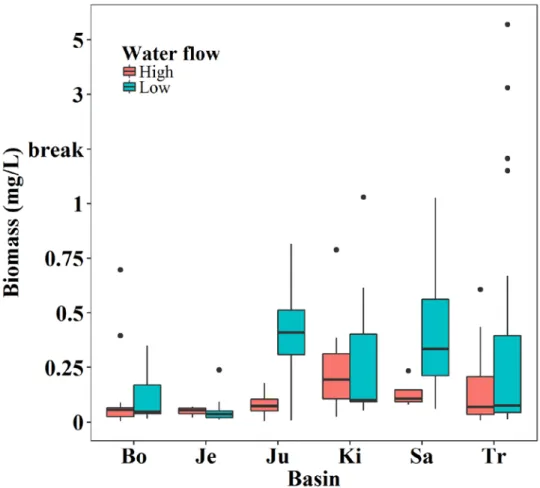
water flow period) and spatial (sub-basins). We also found that biomass increased significantly from
281
high flow to low flow period in the sub-basins of Tr, Sa and Ju, while fewer changes occurred in the
282
sub-basins of Bo, Je and Ki (Fig. 3). In both hydrological periods, functional group TB constituted a
283
high portion in sub-basins: Bo (87% - Dec. 2014, 68% - Sep. 2015) and Je (98% - Dec.2014, 64% -
284
Sep. 2015). In contrast, the functional group M percentage increased in the sub-basin of Tr, Ki, Sa
285
and Ju from December to September (Table A. 2).
286
17 287
Fig. 3 Average biomass in different basins (Bo represents for sub-basin Bollingstedter Au, Je for Jerrisbek, Ju for 288
Juebek, Ki for Kielstau, Sa for Sankermark See and Tr for mainstream of Treene) 289
290
3.3. Effect of abiotic factors on phytoplankton functional groups
291
3.3.1. Relationship described by variation partitioning
292
In wet season (Dec. 2014), there were 3 L, 5 H and 5 P variables selected by a forward selection
293
(supporting information Table A. 3). All the groups showed significant relationships with PFGs (by
294
anova function in R, p<0.001). According to variation partitioning analysis, the three sets could
295
explain 44% of the variation in PFGs (Fig. 4). The variations purely explained by H, L and P were
296
4%, 2% and 6%, respectively, while the shared fraction of the three variables was 14%. In general,
297
the joint contribution by H and P (H×P, 9%) was higher than those by H×L (2%) and P×L (7%). In
298
the dry season (Sep. 2015), there were 2 L, 1 H and 6 P variables selected by a forward selection
299
18
(Table A. 3). The PFGs variation was mostly related to the effect of P (their pure effect explained
300
10% of the variation), whereas the pure effect of H was the least (only accounted for 0.4%). The
301
variation partitioning also showed that both wet and dry periods had similar explanation fraction of
302
land cover (Dec. 2014: 2%; Sep. 2015: 2%).
303
304
Fig. 4 Contributions of the hydrological (H), land-cover (L) and physicochemical (P) variables to the variances in 305
phytoplankton functional groups (PFGs). Each diagram represents a given biological variation partitioned into the 306
pure effects of H, L and P (i.e. when removing the variations caused by other two factors), interaction between any 307
two variables (H×L, L×P, H×P), interaction of all three factors (H×L×P) and unexplained variation (total variation 308
= 100). The analysis includes two scenarios: left: illustrate the situation in December of 2014 (n=59), right: show 309
the results in September of 2015 (n=59).
310 311
3.3.2. Relationships described by structural equation model
312
From the general linear model results (supporting information Table A. 4), we got a general
313
idea about the effects of the multiple stressors. For further investigation of the causal relationship
314
between the abiotic and biotic variables, we fitted structural equation models (SEMs) to infer the
315
direct and indirect effects of specific abiotic variables on bio-indicators (indicated by NMDS1 and
316
phytoplankton functional groups M, TB) (Fig. 5).
317
In high flow period (Dec. 2014), SEMs indicated that group M was directly governed by
318
19
PO43--P and TP (β=0.276, 0.378, respectively, standardized coefficient), while indirectly affected by
319
URMD via PO43--P and TP (β=0.558, -0.448, respectively, standardized coefficient). The
320
hydrological variable H20 (skewness of 7 days’ discharge) was mediated through sulfate (SO42-)
321
effect on TB. The SEM explained 72.8% of the variation of NMDS1. The explanations come from
322
H36 (skewness of 30 days' discharge), PO43--P, TP, SO42- directly, and URMD indirectly via H20.
323
During the low flow period (Sep. 2015), the strongest relationship (β=0.525, standardized
324
coefficient) was observed in the SEM analysis between functional group TB and dissolved oxygen
325
(DO). H20 exerted an indirect effect on TB via DO (β=-0.465, standardized coefficient). Area
326
covered by water (WATR) appeared as the key variable for the group M, directly (β=0.503,
327
standardized coefficient) and indirectly through NPR (β=-0.318, standardized coefficient). The SEM
328
explained 31% of the community variation (represented by NMDS1) was negatively affected by DO,
329
and positively affected by WT and WATR.
330
331
20 332
Fig. 5 Structural equation models embody the causal relationships between hydrological regime (H), land-use 333
pattern (L), physicochemical condition (P) and phytoplankton bio-indicators. Solid arrows represent direct paths 334
(p<0.05), and dashed arrows represent indirect paths. The values corresponding to the path coefficients have 335
standardized effect size. The models are evaluated using R2. The hydrological parameters are in blue squares, 336
physicochemical parameters in green squares, land-use parameters in red squares, and the orange squares represent 337
phytoplankton functional groups (M, TB) and community index (NMDS1). The analysis includes two scenarios:
338
the upper one illustrates the situation in December of 2014 (n=59), the lower one shows the results on September of 339
2015 (n=59). The environmental variables included: H20: skewness of 7 days’ discharge (including the sampling 340
day); H36: skewness of 30 days' discharge (including the sampling day); WATR: area covered by water; URMD:
341
urban area with residential-medium density; PO4: phosphate- phosphorus; TP: total phosphorus; SO4: sulfate; NPR:
342
nitrogen to phosphorus ratio; DO: dissolved oxygen; WT: water temperature.
343 344
4. Discussion
345
4.1. Response of TB to multiple stressors
346
We observed a higher contribution of hydrological regime during high water period (Fig. 4).
347
The result demonstrated the importance of flow regime in shaping phytoplankton community
348
population and composition, which was also supported by previous results in the study region (Qu et
349
21
al., 2018a). Among the hydrological variables, skewness of discharge in 7 days (H20) emerged as the
350
key factor in shaping the pattern of TB both in wet and dry periods of the study (Fig. 5). The index
351
H20 provided two opposite trends across different hydrological periods. One river could present two
352
types of hydrograph on skewness depending on the hydrological conditions, such as in the river
353
Piquiri, South Brazil, where small (large) floods present positive (negative) skewness (Fleischmann
354
et al., 2016). The maximum value of skewness of flow in the studied catchment was observed in the
355
tributary Jerrisbek during the wet season. As we know, the Jerrisbek tributary is in the flatter hill
356
region. Additionally, the region had a higher share of forest and pasture, which turned to interfluvial
357
wetland during flooding, which leads to low flood wave attenuation (Junk et al., 2011). A larger
358
skewness implied higher discharge and runoff variability (Poff and Zimmerman, 2010).
359
Higher percentage of TB was observed in the tributary of Jerrisbek compared to other areas of
360
the river (Table A. 2). The PFG TB as typical potamal phytoplankton better dominated in high flow
361
condition of small rivers (Stanković et al., 2012). The result support the hypothesis that increased
362
water discharge can trigger higher share of TB in the community, due to their relatively high
363
tolerance to flushing and turbulence (Borics et al., 2007). Phytoplankton communities were
364
co-dominated by planktic and benthic algae. The proportion of silicified benthic diatoms increased
365
when water residence time decreased (Beaver et al., 2013). Consistent with this, Wang et al. (2018)
366
demonstrated that the community composition of benthic diatoms in river plankton was not
367
randomly distributed. Additionally, it could be related to algal hydrological constraints based on their
368
morphological and functional traits aspects in a meaningful way. Likewise, B-Béres et al. (2016) also
369
emphasized that the trait of guild was a sensitive indicator for the environmental conditions in the
370
22
lowland rivers and streams.
371
Furthermore, we also observed a significant positive relationship between sulfate and benthic
372
diatoms. The results revealed the possible importance of sulfate for diatoms growth. Based on a
373
controlling experiment, sulfate is likely to be a promotion factor, which would be a benefit to the
374
photosynthetic characteristics of benthic diatoms (Lengyel et al., 2015).
375
4.2. Response of M to multiple stressors
376
During high flow period, domestic area (URMD) is selected as an indirectly structuring factor
377
to M via essential nutrient phosphorus (Droop, 1974), and the soluble phosphate was positive related
378
with M (Fig. 4). It was surprisingly against with our hypotheses that the key factor would be the
379
major land-use of agriculture. However, the results are consistent with other previous findings. In the
380
Taizi River basin (China), they reported the pollution sources from built-up land areas were existing
381
in both rainy and dry seasons as a point source, where the population is dense and industrial activities
382
are intensive (Bu et al., 2014). It was reported that the urbanized land-use had better production of
383
water quality than agricultural land-use, indicating that urbanized land-use is the primary contributor
384
to degraded water quality rather than agricultural land-use (Baker, 2003; Schoonover and Lockaby,
385
2006). Additionally, it was reported a continuous high supplement of nitrogen, while controlled
386
phosphorus in the rural area (Mischke et al., 2011). The condition of phosphorous showed as an
387
important nutrient factor, especially for the growth of M.
388
During the low flow period, the area covered by water body (WATR) appeared as another key
389
factor for controlling the functional group M with a direct positive relationship (Fig. 5). The result
390
indicated that the lake act as a source of Microcystis rather than a sink of purification in the
391
23
catchment. The biomass of the percentage of M was the highest on the sites after lakes. On the
392
contrary, Lake Durowskie (west Poland), which is also located in a farmland-dominant catchment,
393
has suffered inflow with severe cyanobacteria blooms by the linked Struga Gołaniecka River.
394
However, the outflow water quality recovered by three restoration methods in the lake (Gołdyn et al.,
395
2014; Kowalczewska-Madura et al., 2018). As a typical planktic group, M has been regarded as a
396
group with the preference of small, eutrophic lacustrine habitat (Borics et al., 2007), while
397
sensitivities to flushing and low light (Reynolds et al., 2002). In lentic area, high phytoplankton
398
bio-volume may dominate by bloom-forming cyanobacteria occurring due to high water residential
399
time (Rangel et al., 2016). The upstream dam resulted in lake type eutrophic, epilimnetic Microcystis
400
dominance, while replaced by benthic diatoms in the middle sections of the River Loire (France) in
401
late summer (Abonyi et al., 2012).
402
Moreover, we also observed that the ratio of nitrogen to phosphorous was directly negative
403
related to group M during the dry season (Fig. 5). On one hand, the result showed that the content of
404
phosphorous acted as the shaping factor for Microcystis development (Schindler et al., 2016). On the
405
other hand, the negative relationship between NPR and M consistent with the previous studies that
406
cyanobacteria bloom was favored by low NPR (Orihel et al., 2015; Smith, 1983).
407
Finally, we are specially facing a high biomass of M on the low flow period, when local farmers
408
fertilized crops and used pesticides more extensively in the study region (Ulrich et al., 2018).
409
Cyanobacteria had been noticed by higher tolerance to herbicides than other phytoplankton taxa
410
(Bérard et al., 1999), particularly under status of enhanced nutrient supply (Harris and Smith, 2016),
411
indicating pesticides might potentially stimulated the dominance of M during low flow period.
412
24
4.3. Response of phytoplankton community to multiple stressors
413
During the high flow period, the phytoplankton community pattern had a higher influence from
414
hydrological indexes compare to the dry period (Fig. 5). The hydrological regime mainly contributed
415
to the low biomass and high similarity of the phytoplankton composition during the high flow period,
416
due to the high connectivity and extensive dispersal stochasticity (Rodrigues et al., 2018). On the
417
contrary, there was a relative high level of total biomass during the dry season (Fig. 3), and a high
418
share of contribution from physicochemical condition in structuring the phytoplankton community
419
(Fig. 4). Firstly, it can be expected a light limitation in winter months in the Northern Hemisphere. In
420
addition, we could infer even higher light availability in the dry season due to the low water level
421
(Nõges et al., 2016). Moreover, water temperature had a positive contribution to the phytoplankton
422
population development in September (Fig. 5). This phase of the year had more suitable temperature
423
for algae growth compared to December. Warm autumn water temperatures combined with
424
anthropogenic eutrophication attributed to the cause of riverine algal blooms during drought period
425
(Bowling et al., 2016).
426
Overall, our findings suggest that the impacts of flow regime, land-use pattern, physicochemical
427
condition and their potential interactions on riverine PFGs (TB, M and the community) varied
428
greatly across hydrological periods. However, traditional biomonitoring campaigns and management
429
practices, which focused on improving local abiotic variables to increase local biodiversity, were
430
often based on one-time sampling data and fairly ignored the potential bias resulting from temporal
431
variations, particularly different hydrological periods (Stubbington et al., 2017b). The designation
432
was probably one of the reasons that have resulted into many problems and delays in implementation
433
of recent international water framework directive policies such as EU WFD (Voulvoulis et al., 2017).
434
25
We therefore advocate that sampling programs and analyses that target future environmental policies
435
should take different hydrological periods into account (Stubbington et al., 2017a). Furthermore,
436
studies address that detailed causal relationships between changing environment and aquatic
437
organisms could significantly improve our basic understanding of ecological responses to multiple
438
stressors. Sustainable watershed management requires holistic approaches that assess collective
439
biotic and abiotic data to better predict the impacts of anthropogenic activities and climate change on
440
aquatic ecosystems (Dudgeon et al., 2006).
441
5. Conclusions
442
In this study, the phytoplankton biomass and functional groups composition vary
443
spatiotemporally during two contrasting seasonal hydrological periods. Their responses to
444
physicochemical conditions, hydrological regime and land-use pattern are different during different
445
hydrological periods. we detect that:
446
(1) The hydrological regime contributes more during the high flow period in structuring the
447
phytoplankton community. The skewness of 7 days discharge emerged as a key driver of
448
hydrological regime, and it always had an indirect effect on functional group TB during two
449
hydrological periods.
450
(2) Anthropogenic stressor by urban land-use acted as a critical driver for functional group M
451
especially during high flow period. The group M was directly related to phosphorous
452
relevant indicators indicating its sensitivity to the concentration of phosphorous. The area
453
with a higher share of water bodies was also a key cause factor during the low flow period,
454
guide the lacustrine zone as its origin.
455
26
Our results provide evidence that, for a more comprehensive and accurate understanding of the
456
aquatic status, we should also take consideration of different hydrological periods. Secondly, we
457
recommend functional groups as effective indicators of phytoplankton dynamics to simplify the
458
pattern and seize the key issue to achieve a better knowledge of the relationship between
459
phytoplankton and multiple environmental stressors. Climate change and anthropogenic activities,
460
for instance altering flow regime and land-use pattern, act as an important ecological filter of riverine
461
phytoplankton community via physicochemical conditions. Further studies across lake-river
462
continuums are needed to enhance our understanding toward incorporating hydrological regime,
463
land-use pattern, as well as physicochemical conditions into investigation designs, which would
464
enable us to keep the pace with increasing demand for sustainable watershed management. Structure
465
equation model disentangled the contribution of multiple stressors. It would be an outperforming
466
method to generalize results, identify common patterns, and predict response of phytoplankton to
467
environmental changes in future studies.
468
Acknowledgments
469
This study has funded by German Research Foundation (Deutsche Forschungsgemeinschaft DFG)
470
grants (FO 301/15-1, FO 301/15-2, WU 749/1-1, WU 749/1-2, and the project GU 1466/1-1
471
Hydrological Consistency in Modelling). There is financial support scholarship by AIAS CO-FUND
472
funding (Naicheng Wu) and China Scholarship Council (CSC) (Yueming Qu). We thank: Dr. Fuqiang
473
Li, Zhao Pan and other friends for their support during the field campaigns, and the laboratory team
474
of the Department of Hydrology and Water Resources Management of the Christian Albrechts
475
University of Kiel for carrying out the water quality analysis. We also thank Ms. Rebecca Pederson for 476
27
help to revise the language problems. The valuable comments of two anonymous reviewers have 477
improved the manuscript greatly.
478
References
479
Abonyi, A., Leitao, M., Lançon, A.M., Padisák, J., 2012. Phytoplankton functional groups as indicators of human impacts 480
along the River Loire (France). Hydrobiologia 698, 233-249.
481
B-Béres, V., Lukács, Á., Török, P., Kókai, Z., Novák, Z., T-Krasznai, E., Tóthmérész, B., Bácsi, I., 2016. Combined 482
eco-morphological functional groups are reliable indicators of colonisation processes of benthic diatom assemblages 483
in a lowland stream. Ecological Indicators 64, 31-38.
484
Bąk, M., Witkowski, A., Żelazna-Wieczorek, J., Wojtal, A., Szczepocka, E., Szulc, K., Szulc, B., 2012. Klucz do 485
oznaczania okrzemek w fitobentosie na potrzeby oceny stanu ekologicznego wód powierzchniowych w Polsce.
486
Biblioteka Monitoringu środowiska.
487
Baker, A., 2003. Land use and water quality. Hydrological processes 17, 2499-2501.
488
Beaver, J.R., Jensen, D.E., Casamatta, D.A., Tausz, C.E., Scotese, K.C., Buccier, K.M., Teacher, C.E., Rosati, T.C., 489
Minerovic, A.D., Renicker, T.R., 2013. Response of phytoplankton and zooplankton communities in six reservoirs 490
of the middle Missouri River (USA) to drought conditions and a major flood event. Hydrobiologia 705, 173-189.
491
Bérard, A., Leboulanger, C., Pelte, T., 1999. Tolerance of Oscillatoria limnetica Lemmermann to atrazine in natural 492
phytoplankton populations and in pure culture: influence of season and temperature. Archives of environmental 493
contamination and toxicology 37, 472-479.
494
Bergström, A.-K., 2010. The use of TN: TP and DIN: TP ratios as indicators for phytoplankton nutrient limitation in 495
oligotrophic lakes affected by N deposition. Aquatic Sciences 72, 277-281.
496
Bey, M., Ector, L., 2013. Atlas des diatomées des cours d’eau de la région Rhône-Alpes. Cent de Rech Public 2, 181-331.
497
Blanchet, F.G., Legendre, P., Borcard, D., 2008. Forward selection of explanatory variables. Ecology 89, 2623-2632.
498
Bolgovics, Á., Várbíró, G., Ács, É., Trábert, Z., Kiss, K.T., Pozderka, V., Görgényi, J., Boda, P., Lukács, B.-A., 499
Nagy-László, Z., 2017. Phytoplankton of rhithral rivers: its origin, diversity and possible use for quality-assessment.
500
Ecological Indicators 81, 587-596.
501
Borcard, D., Legendre, P., Drapeau, P., 1992. Partialling out the Spatial Component of Ecological Variation. Ecology 73, 502
1045-1055.
503
Borics, G., Várbíró, G., Grigorszky, I., Krasznai, E., Szabó, S., Kiss, K., 2007. A new evaluation technique of 504
potamo-plankton for the assessment of the ecological status of rivers. Archiv für Hydrobiologie (Supplement) 161, 505
465-486.
506
Bowling, L., Egan, S., Holliday, J., Honeyman, G., 2016. Did spatial and temporal variations in water quality influence 507
cyanobacterial abundance, community composition and cell size in the Murray River, Australia during a 508
drought-affected low-flow summer? Hydrobiologia 765, 359-377.
509
Bu, H., Meng, W., Zhang, Y., Wan, J., 2014. Relationships between land use patterns and water quality in the Taizi River 510
basin, China. Ecological Indicators 41, 187-197.
511
Burchardt, L., 2014. Key to Identification of Phytoplankton Species in Lakes and Rivers: Guide for Laboratory Classes 512
and Field Research. W. Szafer Institute of Botany, Polish Academy of Sciences.
513
28
Bussi, G., Whitehead, P.G., Bowes, M.J., Read, D.S., Prudhomme, C., Dadson, S.J., 2016. Impacts of climate change, 514
land-use change and phosphorus reduction on phytoplankton in the River Thames (UK). Science of the Total 515
Environment 572, 1507-1519.
516
Devercelli, M., 2006. Phytoplankton of the Middle Paraná River during an anomalous hydrological period: a 517
morphological and functional approach. Hydrobiologia 563, 465-478.
518
Droop, M., 1974. The nutrient status of algal cells in continuous culture. Journal of the Marine Biological Association of 519
the United Kingdom 54, 825-855.
520
Dudgeon, D., Arthington, A.H., Gessner, M.O., Kawabata, Z., Knowler, D.J., Leveque, C., Naiman, R.J., Prieur-Richard, 521
A.H., Soto, D., Stiassny, M.L., Sullivan, C.A., 2006. Freshwater biodiversity: importance, threats, status and 522
conservation challenges. Biological Reviews 81, 163-182.
523
EC, 2000. European Commission Directive 2000/60/EC of the European Parliament and of the Council of 23 October 524
2000 establishing a framework for Community action in the field of water policy. Off. J. Eur. Commun., Brussels 525
L327.
526
Federation, W.E., Association, A.P.H., 2005. Standard methods for the examination of water and wastewater. American 527
Public Health Association (APHA): Washington, DC, USA.
528
Fleischmann, A.S., Paiva, R.C., Collischonn, W., Sorribas, M.V., Pontes, P.R., 2016. On river‐floodplain interaction and 529
hydrograph skewness. Water Resources Research 52, 7615-7630.
530
Gołdyn, R., Podsiadłowski, S., Dondajewska, R., Kozak, A., 2014. The sustainable restoration of lakes—towards the 531
challenges of the Water Framework Directive. Ecohydrology & Hydrobiology 14, 68-74.
532
Grace, J.B., 2006. Structural equation modeling and natural systems. Cambridge University Press.
533
Guse, B., Kail, J., Radinger, J., Schröder, M., Kiesel, J., Hering, D., Wolter, C., Fohrer, N., 2015a. Eco-hydrologic model 534
cascades: Simulating land use and climate change impacts on hydrology, hydraulics and habitats for fish and 535
macroinvertebrates. Science of The Total Environment 533, 542-556.
536
Guse, B., Pfannerstill, M., Fohrer, N., 2015b. Dynamic Modelling of Land Use Change Impacts on Nitrate Loads in 537
Rivers. Environmental Processes 2, 575-592.
538
Haas, M.B., Guse, B., Pfannerstill, M., Fohrer, N., 2016. A joined multi-metric calibration of river discharge and nitrate 539
loads with different performance measures. Journal of Hydrology 536, 534-545.
540
Harris, T.D., Smith, V.H., 2016. Do persistent organic pollutants stimulate cyanobacterial blooms? Inland Waters 6, 541
124-130.
542
Hilton, J., O'Hare, M., Bowes, M.J., Jones, J.I., 2006. How green is my river? A new paradigm of eutrophication in 543
rivers. Science of the Total Environment 365, 66-83.
544
Hofmann, G., Werum, M., Lange-Bertalot, H., 2011. Diatomeen im Süßwasser-Benthos von Mitteleuropa:
545
Bestimmungsflora Kieselalgen für die ökologische Praxis: über 700 der häufigsten Arten und ihre Ökologie. ARG 546
Gantner.
547
Hu, H., Wei, Y., 2006. The freshwater algae of China: systematic, taxonomy and ecology. Science Press, Beijing.
548
Huang, X.F., 2000. Survey, observation and analysis of lake ecology. Standard Press of China, Beijing.
549
Junk, W.J., Piedade, M.T.F., Schöngart, J., Cohn-Haft, M., Adeney, J.M., Wittmann, F., 2011. A classification of major 550
naturally-occurring Amazonian lowland wetlands. Wetlands 31, 623-640.
551
Katsiapi, M., Mazaris, A.D., Charalampous, E., Moustaka-Gouni, M., 2012. Watershed land use types as drivers of 552
freshwater phytoplankton structure. Hydrobiologia 698, 121-131.
553
Kiesel, J., Fohrer, N., Schmalz, B., White, M.J., 2010. Incorporating landscape depressions and tile drainages of a 554
northern German lowland catchment into a semi-distributed model. Hydrological Processes 24, 1472-1486.
555
Kiesel, J., Guse, B., Pfannerstill, M., Kakouei, K., Jähnig, S.C., Fohrer, N., 2017. Improving hydrological model 556
optimization for riverine species. Ecological Indicators 80, 376-385.
557