Entity-level stream classification: exploiting entity similarity to label the future observations referring to an entity

(1)

https://doi.org/10.1007/s41060-019-00177-1 R E G U L A R P A P E R

Entity-level stream classification: exploiting entity similarity to label the future observations referring to an entity

Vishnu Unnikrishnan¹ ·Christian Beyer¹·Pawel Matuszyk¹·Uli Niemann¹·Rüdiger Pryss²·Winfried Schlee³· Eirini Ntoutsi⁴·Myra Spiliopoulou¹

Received: 2 January 2019 / Accepted: 7 February 2019

Abstract

Stream classification algorithms traditionally treat arriving instances as independent. However, in many applications, the arriving examples may depend on the “entity” that generated them, e.g. in product reviews or in the interactions of users with an application server. In this study, we investigate the potential of this dependency by partitioning the original stream of instances/“observations” intoentity-centric substreamsand by incorporating entity-specific information into the learning model. We propose ak-nearest-neighbour-inspired stream classification approach, in which the label of an arriving observation is predicted by exploiting knowledge on the observations belonging to this entity and to entities similar to it. For the computation of entity similarity, we consider knowledge about the observations and knowledge about the entity, potentially from a domain/feature space different from that in which predictions are made. To distinguish between cases where this knowledge transfer is beneficial for stream classification and cases where the knowledge on the entities does not contribute to classifying the observations, we also propose a heuristic approach based on random sampling of substreams usingkRandom Entities (kRE). Our learning scenario is not fully supervised: after acquiring labels for the initialmobservations of each entity, we assume that no additional labels arrive and attempt to predict the labels of near-future and far-future observations from that initial seed. We report on our findings from three datasets.

Keywords Stream classification·kNN·Entity similarity

We use the termsobservationsandinstancesinterchangeably, since we speak of a time series of property values that exist at all times but are observed at different points in time.

B

Vishnu Unnikrishnan vishnu.unnikrishnan@ovgu.de Christian Beyer

christian.beyer@ovgu.de Pawel Matuszyk

matuszyk.pawel@googlemail.com Uli Niemann

uli.niemann@ovgu.de Rüdiger Pryss

ruediger.pryss@uni-ulm.de Winfried Schlee

winfried.schlee@klinik.uni-regensburg.de Eirini Ntoutsi

ntoutsi@kbs.uni-hannover.de Myra Spiliopoulou

myra@ovgu.de

1 Introduction

Most data sources analysed for decision making are of a dynamic nature. Purchases, reviews and ratings are subject to changes in customers’ attitudes and in products’ popu- larities. User interaction with mobile apps and social media reflects the people’s changes in interests, preferences and mood. Stream classification algorithms treat streaming data as data/observations that arrive independently. This seems oversimplifying, since the sales of a specific product or the recordings of a patient interacting with an mHealth app certainly depend on the associated entity—the product or patient. So, it is reasonable to expect that information on the

1 Otto-von-Guericke Univeristy Magdeburg, Magdeburg, Germany

2 University Ulm, Ulm, Germany

3 University Hospital Regensburg, Regensburg, Germany

4 Leibniz University Hannover, Hannover, Germany

(2)

specific data-generating entity and on other entities (products, patients) that the query entity is similar to can improve model quality. For instance, predicting future blood glucose levels for a diabetic patient may benefit from considering other, similar patients with diabetes. This approach is also potentially useful given that most real-world applications have to deal with data sparsity issues, and inferring information from the neighbourhood may improve the quality of predictions. Towards this end, we propose a neighbourhood- based approach that trains entity-specific stream classifiers and exploits similarity among entities for learning, rather than similarity among the individual instances comprising them, i.e. the entity is assumed to have both static and dynamicinformation associated with it, and the static information is used to compute the similarity neighbourhood, while information from similar entities is exploited to make predictions in the dynamic space.

There are abundant advances in stream classification, as reflected in recent surveys like [6,13], where major challenges are identified, including the non-stationarity of the data-generating process and the need to learn and adapt the model efficiently. Although ensembles are seen as a very competitive learning paradigm for stream classification [13], the idea of learning entity-specific models has received little attention in stream learning [3], in contrast to the obvious entity-centric learning in time series analysis (where each time series, usually generated by an entity, is treated sep- arately from those generated by others). In our work, we attempt to bring the two fields closer by exploiting the his- tory of an entity and that of entities similar to it to predict the labels of the arriving observations.

Similarity among entities is traditionally exploited in time- series analysis, and many extensions have been proposed since the introduction of the first principles (cf. [28] for one of the early papers). The core idea is to compare the series of observations appertaining to different entities, thereby using dynamic time warping and its variants to align time series of different lengths [11]. However, this idea does not transfer to the context of entity-centric learning on a stream for two reasons. First, there is no reason to suppose that the observations on two independent entities will arrive at the same speed. For example, if during a period of 24 months a patient (entity) has been inspected by a physician twice (two observations), while another patient has been inspected 24 times (e.g. once per month), it seems inappropriate to align these two time series. Second, time series are finite, so each observation in them can be labelled, while streams are infinite.

Hence, the assumption of a constantly available oracle that supplies fresh labels on demand must be questioned. Solu- tions should therefore be developed that take into account the fact that different entities are tracked at different rates, and that labels may not always be available.

In this work, we propose an entity-centric stream classification method that predicts the labels of the observations belonging to an entity without requiring that the streams of the individual entities have similar speeds, and without demanding that fresh labels are made available at any time by an oracle. To achieve this, we transfer similarity information among entities from a static domain, and we learn on an initial, small set of labelled observations, assuming that no labels arrive thereafter. We investigate how far in the future of each entity we can predict, given this limited amount of labelled data.

Our approach encompasses the following components:

an entity-level classifier for numerical data (i.e. a regressor), a method for computingk-nearest neighbours (kNN), a baseline method for computing predictions usingkRan- dom Entities (kRE) and comparing the learners in order to reject irrelevant domains (from the transfer), and a method for building a predictive subspace for a domain. We investigate our approach on three datasets: patients interacting with an mHealth app, product reviews, and sensor data on air quality. Since the predicted labels in this study are numeric, kNN predictions are evaluated on RMSE and compared against that from the kRE model.

It is to be noted that our proposed method does not use kNN as a classifier, and more as a tool mitigating label sparsity for an entity by expanding to its neighbourhood. Our approach also differs from kNN-based regression, because the feature space in which kNN is computed is not the feature space seen by the classifier making the predictions.

The paper is organised as follows. The next Sect.2dis- cusses related work, and the following Sect.3describes the proposed workflow. In Sect. 4we present our experiments and discuss our findings, before closing in Sect. 5 with a summary and outlook.

2 Related work

In our recent work [3], we propose an entity-centric learning approach for opinionated document streams. We compare the performance of a classifier trained on all opinionated texts to that of classifiers that see only the data associated to the entity itself, and show that in some cases even basic entity- centric models achieve competitive performance. However, this approach ignores all variables except the document label (prediction using only timestamp, and ‘without reading con- tent’ of the arriving instances). Here, we build upon this conceptual model but exploit further timestamped data, while we do not assume label availability beyond the first few observations per entity.

(3)

2.1 kNN-based predictions in time series data The task of prediction over a sequence of observations for an entity is addressed in the context of time series analysis, where kNN is used to identify an entity’s nearest neighbours and exploit them for learning. In [2], Ban et al. use a kNN-based regression method to predict future values of stock prices. The fundamental assumption is based on economic intuition from [5] that within-industry returns cor- relate highly compared to cross-industry returns. A two-tier, multivariate regression method for financial time series forecasting is used to exploit this fact. The first step computes the nearest neighbour for each entity (companies belonging to S&P500, in this case) based on degree of correlation over historical data, and the next step builds a multivariate regressor to predict future values using each of the neighbours identified.

This two-step approach of first identifying neighbours and then learning on them is an idea that is very close to what we propose. However, the chief difference in our approach is that unlike in [2], we do not assume that all time series have equal lengths. In addition, the dataset in [2] subsets the S&P500 to select stocks from four sectors, while we do not subset the original set of time series.

Several papers ([18,19,26], and [17]) assess the efficacy of kNN-based systems in forecasting electricity prices. The works of both [1] and [19] adapt a method very similar to that in [2] for prediction of electricity prices (in the UK and Spain, respectively). For this prediction task, each day’s electricity price information is stored as a 24-value time series (one observation per hour). The neighbours are discovered with kNN using Euclidean distance. Since all time series are aligned and of equal length, more sophisticated distance functions are not necessary. The methodology in [1] improves on the shortcomings of [19], where the time series are pre- processed to exclude weekends and holidays. This is done by using multiple regression to forecast prices while accom- modating additional variables like temperature, cloudcover, wind chill, etc., and dummy variables to flag holidays and weekends.

2.2 Time series prediction with deep learning algorithms

Time series prediction with help of deep learning algorithms is enjoying increasing attention. This invites the question of whether simplistic kNN-based approaches are still an appropriate first choice for predicting the label of the next observation of an entity. In their “Review of Unsupervised Feature Learning and Deep Learning for Time Series Model- ing” [15], Längkvist et al. state that “Time series data consists of sampled data points taken from a continuous, real-valued

process over time.” This rather obvious statement is reflected in modelling and analysis of time series of observations generated by a set of entities, e.g. flow of crowds from different residual units inside a city [29], or flow of vehicles [21].

In our research context, the statement of [15] is not guaranteed to hold: it would be rather surprising if the opinions on all products belonging to the same category (e.g.

watches) would adhere to the same data-generating process.

Similarly, patients with the same disease but with different static characteristics like birthdate, sex, and time since disease onset, and with different comorbidities, should not be assumed to generate observations according to the same overarching process. Hence, an exploitation of the static information on the entities seems essential next to the timestamped data. Studies on the use of clinical recordings, e.g.

for predicting the outcome of an intervention [25], take also patient static data into account, including phenotypes and lab tests.

Given the availability of both static and timestamped data, it seems most appropriate to use advanced machine learning algorithms that can exploit both. However, the streams of the individual entities may vary substantially on the number of observations per entity. This corresponds to time series of different lengths per time frame, since streams are endless time series. The authors of [4] use recurrent neural networks for predicting time series with missing values within each time frame. This approach seems promising for entities that have a comparable total number of observations. However, we concentrate on predictions after acquiring a minimal number of observations per entity, without making assumptions on the time frame in which they arrive.

2.3 Label prediction under infinite verification latency

Conventional stream classification algorithms assume that an oracle (e.g. a human expert) provides a label for each arriving observation. The temporary unavailability of the oracle, i.e.

theverification latencyleads to semi-supervised and active learning solutions for stream classification [14]. If there are no new labels at all, i.e. in the case of infinite verification latency, semi-supervised stream classification methods are employed, see, e.g. [7,27]. These methods have been designed for a single stream of observations though, not for entity-centric streams.

In the domain of time series prediction, semi-supervised algorithms are less widespread. Short-term prediction in the stock exchange market with help of semi-supervised algorithms is proposed in [12]. In our work, we do not transfer derived labels, as in semi-supervised learning, but similarity information from another domain, and consider this information for short-term and long-term predictions.

(4)

2.4 Short- and long-range forecasting

Recent work has also called into attention the need for short- and long-term forecasts for time series under various constraints like missing values, etc. [8] proposes forecasting methods for cross-sectional observations of multiple multivariate time series and makes the distinction between

‘Continuous Approach’esand‘Distance Approach’es. Con- tinuous methods use already forecasted values to make forecasts farther in the future (like ARIMA), and distance methods do not. The latter is handled by varying the ‘target cross section’ (the time at which the cross-sectional observation of all time series are made) while holding the rest of the data constant. This is close to what we propose in this work, but is subtly different from our approach, since our work focuses on using all variables except the class label from the multivariate time series when making a short- or long-range forecast.

3 Neighbourhood-assisted predictions

This work postulates that while making predictions for observations of an entity, observations of entities that fall in its neighbourhood can be leveraged to improve predictions. This involves three steps: finding the neighbours of an entity, choosing how to learn models on data of the entity and its neighbours, and combining each model’s prediction to create a final prediction. As already described in Sect.1, we generalise the notion of an entity here to something that has bothstatic properties(like the age, gender of a patient) and dynamic properties(like daily blood sugar levels). This has the consequence that neighbour discovery can work on a set of attributes that are outside the dynamic attribute space. In the following parts of this section, Sect.3.1provides a more formal definition of the problem we aim to solve. Section 3.2describes how the similarity between two entities can be defined in a feature space other than that where the predictions are made. Section3.3describes the various options available for dealing with timestamps while combining data from individual entities. Subsequently, Sects.3.4 and 3.5 describe how predictions are made from entity data augmented with neighbourhoods, and how these neighbourhoods can be pruned to excludefalse neighbours.

3.1 Formalisation of the prediction problem

We study a stream of instances linked to predefined entities, and we investigate the problem of predicting the labels of arriving observations, given static information on the entities, next to the observations themselves. We formalise this problem as follows.

AssumeEbe a set of entities, the static properties of which are expressed in attribute space Do, while the observations on each entitye∈ Econstitute an “entity-centric” streamTe

over the domain-specific attribute spaceDp. An observation arrives at a time pointtj, so that the total number of observations attj is j. For an entitye, the number of observations seen untiltj constitutes the “entity length” (or “length”) of eat tj,length(e,tj)and is upper bounded by j and lower bounded by zero.

The supervised learning goal over this stream would be to label the observation arriving attj, given the past observations and a fixed set of labelsL. Rather, assume that the oracle which provides the labels delivers an initial set of labels, namely for the firstmobservations for each entity. After this seed of labelled observations, no more labels arrive, i.e. the oracle is no longer available. Then, the classification problem is as follows: for each entityeand observationoe,j on e, with j >m, predict the label ofoe,j.

In this study, we concentrate on numerical labels only.

Our approach does not propagate labels, as in typical semi- supervised stream learning, but rather focuses on predicting the labels for j >mgiven the firstmlabels per entity and the static information on the entities from Do. In our experiments, we investigate how prediction performance changes as jmoves fromm+1 towards values much larger thanm.

For our prediction task, we consider following steps: (a) computing an entity’s neighbourhood in domain Do—with kNN; (b) using this neighbourhood to inform the model of an entitye, by finding a suitable way to augment this data; (c) using the model for prediction—in thenear futureand in the far future, requiring a specification of what is near and what is far in the future. The following parts of this section detail the various components that the various subtasks detailed above.

3.2 Borrowing an entity’s neighbours from another domain

For a given domain Do with feature space F, we specify the notion of similarity between entities, compute an entity’s nearest neighbours and verify whether these neighbours lead to better performance than randomly selected entities. This means that for each entitye, the nearest-neighbour computation is performed on attribute spaceDo, but supplemented with aggregated information from the time series attribute space Dp. For example, if predictions are being made for blood sugarvalues (a variable inDpspace), then theaverage of the training-set blood sugar value for the entity in question can be added as one of the features inDo. Ideally, this would mitigate the problem that kNN can compute neighbourhoods in Do with no regard to the values of prediction interest in Dp. These steps to include information fromDoin the neighbourhood computation can be seen asborrowingthe notion of similarity from domain Doto improve the predictions in

(5)

domainDp. The use of aggregated information helps mitigate the problems created by computing similarities for time series of very different lengths, and/or those with large gaps.

We explore the simplest case by including the aggregated value only for the variable of prediction interest fromDp(i.e.

only one of the variables fromDp, the one for which we make predictions is included along withDo). The nearest neighbours of an entity are computed using the kNN algorithm.

We only use Euclidean distance in this work, and the distance between two entities is defined as the total distance between the values for each of their relevant attributes weighting all attributes equally. As already discussed, the attributes used may be a subset of the total attributes available. The optimal value ofkis discovered experimentally. However, Euclidean distance can be replaced with other distance functions.

3.2.1 Selecting a predictive subspace overD_o

An optional step before applying kNN would be to select from the list of available features inDo, the ones most suited for the prediction task for the variable of interest inDp. The feature selection step is guided either by human intuition, or is discovered in a way that maximises performance. It is clear that manual feature selection is only feasible in cases that Dodoes not have a large number of variables, and the dependencies between variables inDoandDpare intuitive (e.g. the inclusion ofstressas a variable that affects tinnitus).

We propose a solution that simultaneously optimises the selected features and evaluates the quality of the selected feature space, using an evolutionary algorithm. Each individual in the evolutionary algorithm is a Boolean vector Vi, with i ∈ 1. . .|Do|. The fitness of each individual is the performance of the model built on the neighbourhood defined by the features that hadVi =T r ue,i∈1. . .|Do|.

3.2.2 Testing the relevance ofD_oby building a model from random entities

The main assumption of this work is that for a set of entities E, each of which consists of static, unchanging attributes in an attribute space Do, and a sequence of timestamped observationsoi1. . .oi t of arbitrary length in attribute space Dp, the ‘neighbourhood’ of an entity in Docan inform on the future observations of the entity (in space Dp). Most existing work optimises for the neighbourhood sizek, but does not verify whether the specific neighbourhood chosen is responsible for the low errors. We therefore propose a novel method for evaluating the contribution of the neighbourhood towards prediction—for a givenk and particular entityep, we pickkRandom Entitieser1. . .er k, and build a regression model on each, as detailed in Sect.3.4. It is expected that this will show the degree to which the neighbourhood improves prediction.

3.3 Time alignment inD_p

The kNN step provides a list of similar entities for each entity e. However, a model can be learned on the entities in the neighbourhood ofeeither by time-aligning each entity’s first observation to time 0, or to preserve the global time in the dataset as is. This can help understand if the global time in the dataset can inform on the tendencies of an entity, or whether the model parameters depend only on an entity’s own past (relative time w.r.t. entity), and not the exact time at which the observations were made.

To investigate the effect of the global, dataset-level

‘clock’, we investigate two variants of treating the obser- vationsoz ∈ ep ∈ E. The first variant is a ‘global clock’, which uses this timestamp of each observationoias-is, without any modification. The second variant gives each entity a

‘local clock’, which begins with the first observation arriving for that entity, i.e. we pre-process the observation time stamps so aligned_ti mestamp(oz) = ti mestamp(oz)− mi n_ti mestamp(ep). The details of how a model can be built on data from either variant is detailed in the following Sect.3.4.

3.4 Creating augmented regressors

Once the kNN step is complete, the prediction for an entity ep can be made using the entities ei,i ∈ 1. . .k, where ei ∈ k N N(ep)andi = p or in case of the random base- lineei ∈k R E(ep)andi = p. For eachei(with an arbitrary number of observationst), we have a sequence of observa- tionsoi1. . .oi tin the feature space Dp, over which a model can be learned. In this early exploratory work, we use the first mobservationsoi from entityei to train a linear regression model. We also investigate two ways to combine the data from the entities in the neighbourhood.

Model augmentation The first method trains a linear regression modelmi on each of the entitiesei ∈ k N N(ep), and averages the parametersme,slopeandme,i nt er ceptfor each of the models to create a final model. The RMSE is then computed on predictions made for test observations fore. This method is analogous to learning the tendencies for each entity in the neighbourhood (including the entity itself), and aver- aging all the tendencies to make a prediction for the entity in question. This method is referred to asmodel augmentation.

Data augmentation for regression Since our time series can differ in length and have large gaps, we also propose a method to retain model quality in the case that there are too few observations to learn a reliable model on entityepand/or entities ei ∈ k N N(ep). We propose pooling all observations into a

(6)

setoall such thatoall =

oi∀o ∈ ei. Since we train one common model on the pooled observations from the entire neighbourhood, the problems with gaps and unequal lengths can be mitigated to some extent. This method is calleddata augmentation. In case of the random baseline, everything stays the same but we useei ∈k R E(ep)instead.

Model Retraining In this early work, we always build our linear regression models on the firstmobservations belonging toep. The regression models are not updated after a new observation belonging toeparrives, but we do plan to investigate in this direction in the future.

3.5 Neighbourhood-pruning

The idea that the kNN algorithm might not always find the optimal neighbourhood, thereby leading to suboptimal predictions is described in [19]. Though it is possible to examine data inDpto exclude two entitieseiandej that are in close proximity in the Do space, in this work we attempt to use domain knowledge to guide the kNN algorithm by excluding certain entities from each other’s neighbourhoods. Experts can exploit information inDoto inform the kNN algorithm that entitiesei andej should be excluded from each others’

neighbourhoods even though their data inDoare very similar. For example, the medical expert can provide the intuition that people with type 1 and type 2 diabetes are fundamen- tally different, even though they may both have similarly high values for blood sugar.

In this work, we use neighbourhood pruning on the mHealth dataset, where we exploit the discrepancy between tinnitus loudness and tinnitus annoyance. Tinnitus loudness is the severity of the symptom, whileannoyanceordistress is the psychological effect it has on the patient. It has been noted by in [9] that there is a subset of patients where the loudness of tinnitus and the psychological annoyance that the patient suffers show are discordant. The degree of psychological annoyance due to tinnitus is measured using the Mini-TQ questionnaire, which consists of a 12-question questionnaire with answers in the scale of 0–2 (higher values are worse). To measure the loudness level of the tinnitus symptom, Hiller and Goebel use the Glockhoff and Lindblom’s loudness grad- ing system. They have noted that of the tinnitus patients, about a third have low annoyance scores in spite of high loudness levels. In addition, they have found a ‘specific psychological profile’ that characterises high-annoyance tinnitus sufferers, for example, not feeling low/depressed, not feeling like a victim of their noises, etc., were all predictors of low annoyance even in patients of high loudness [9].

This work investigates if the ‘psychological profiles’

found by Hiller and Goebels may be found in the mHealth

dataset. To this effect, we investigate whether the neighbourhoods in the kNN algorithm may be restricted to subgroups that may be similar in their perception of annoyance given a particular loudness.

We do not investigate this case for the AQI and Amazon datasets because the concept of what constitutes afalse neigh- bouris less clearly defined. However, in the abstract sense, it is possible to exlude certain products from each others’

neighbourhoods. For example, a cheap knock-off of a luxury watch should not be allowed to be in the neighbourhood of the original product, or two air quality sensors should not be in each others’ neighbourhoods if separated by a relatively small distance but fall on different sides of a mountain range trapping ambient pollution on one side.

4 Experiments

Goal of our experiments is to study the performance of our method for the prediction of the labels of observations.

We concentrate on studying the predictive power achieved through the exploitation of entity similarity, and hence focus on prediction rather than adaption. We partition each dataset into an early part used for learning (first 60% of each entity’s time series) and the subsequent part used for testing.

As part of the evaluation, we performnearandfarpredic- tions, predicting the labels of the first N%, and respectively, the last N% of the test data. In a real scenario, the first N%

of the observations would correspond to the first time win- dow, after which the classifier would need to be adapted.

The far predictions are used for gauging model quality, since we expect that a model would perform better in the near future than in the far future. All predictions are measured by root-mean-squared error (RMSE) against the true values, and performance improvement from kNN is compared against thekRandom Entities (kRE) introduced in Sect.3.2.2. The RMSE reported in the experiments is computed over all the predictions made for each observation in each entity’s test trajectory. The RMSE may be computed only for the first part of this test trajectory, as in the case of the first N%, or only for the last part of the test trajectory, as in the case of the last N%.

4.1 Datasets

We consider three datasets: one from the domain of environ- ment monitoring, in which the entities are sensors; one from the domain of mHealth, where the entities are patients interacting with a mobile app; one from e-commerce, where the entities are products on which opinions have been submitted.

For each of the datasets, we remove entities that have too few observations to learn, and then build a train and test set

(7)

from each of the trajectories (time series) of the remaining entities. For each entityeremaining in the dataset after the filtering step, we use the first 60% of the data for training the augmented regressor, and the remaining data for testing.

AQI—yearly EPA carbon monoxide datasets: These are public domain dedicated datasets collected by the US Environmental Protection Agency. The two datasets used in this study are the daily and the yearly carbon monoxide summaries, containing the daily and yearly observations, respectively. The daily carbon monoxide (CO) summaries contain daily observed information for mean CO levels at different sites located all across the US. In addition to CO levels, various other metrics are also available (PM2.5, PM10, etc.), though this work focuses on predictions for CO levels only. However, the ‘Air Quality Index’ (AQI) and the dailyMax_Observed_CO_Valueinformation are also used at the daily level. The selection of attributes was done in a way that balances relevance to the prediction variable as well as data quality. The dataset consists of 200 entities, with 577482 observations for the period from 1990 to 2017. The prediction variable is the mean CO values observed in ppm as measured daily, and has the following values:aver age=0.742,mi n=0.004,max=8.461 and standar d_devi ati on=0.519.

Attribute Space Dofor kNN computation:The yearly CO summary dataset gives the average CO levels observed at these sites over the whole year. In addition to the yearly average observed CO, we also use the latitude and longitude of the measuring site, the standard deviation of the measure- ment, the first and second max values encountered, as well as 90th and 50th percentile values.

Feature selection: For both the daily and the yearly datasets, we removed several variables to focus only on those associated with CO levels. Whenever a particular measuring site had more than one device measuring CO levels, only measurements from the primary device were used. It was also seen that several observations were possible within the day, with average CO levels computed over varying time intervals.

In this case, we kept only the average CO levels measured over the longest time. The attribute space Dp therefore has 3 variables (the timestamp, AQI, and max_CO_Value).

The daily CO level dataset contains data between 1990 and 2017, while for the yearly summary we only keep data from 1989.

Figure1 shows the distribution of entity lengths in the AQI dataset. Note that while there is indeed a large range of lengths, the distribution of #entities for varying entity lengths is not as skewed as in the other datasets.

mHealth dataset: The mHealth dataset is not public domain. It contains data on patients interacting with an mHealth app calledTrackYourTinnitus, to which they enter data several times a day. The feature space of the entity trajectories contains seven variables, one of which captures the

Fig. 1 AQI: #Entities (Y-axis) for various entity lengths (X-axis)

Fig. 2 mHealth: #Entities (Y-axis) for various entity lengths (X-axis)

patient’s overall state of health at the moment of the observation. This variable is numeric with a value between [0,1], and we use it as target variable. For patient similarity, we use an additional dataset that contains 31 variables on the patients themselves (including sociodemographics and symptoms of the disease). We use this second dataset as Do. The data from this application has already been used to create mean- ingful insights, like in [22], which has studied the difference between prospective and retrospective ratings on theTrack- YourTinnitusmHealth platform.

Attribute Space Do for kNN computation:The attribute space for the kNN computation is quite large, and the discovery of the best subspace over which the kNN could be built was done using a genetic algorithm, as discussed in 3.2.1.

Feature Selection:From the list of features available in Dp, all features were used to train the regression model.

All entities with less than five observations were removed, leaving a total of 516 entities in the dataset. A histogram of entity lengths is given in Fig.2.

Amazon—the tools & home improvement dataset:This is a subset of the Amazon product reviews dataset introduced

(8)

in [20], including only reviews for products belonging to the category ‘Tools & Home Improvement’. Only the review star rating, review timestamp, review text, and productID information is exploited from this dataset. The productID and review text combine to formDowith the timestamp and star rating forming theDp. The star rating is the prediction variable, and takes values 1, 2, 3, 4 or 5.

The minimum cutoff for the Amazon dataset was set at least 2 reviews. As can be seen in Fig.3, the skew in entity lengths is rather extreme in the Amazon dataset, with the 25th percentile, 50th percentile, and the 100th percentile being 2, 4 and 4770, respectively. There are 139508 entities in the dataset after filtering, with a mean entity length of 12.9. In addition, [3] has also noted that the most reviews in the dataset cluster towards the last timestamps, along with an increased bias towards high ratings.

Attribute Space Dofor kNN computation:Since the Ama- zon dataset provides no clear set of variables inDoregarding the static properties of the product, we use an aggregated version of the information in the domain Dp. Toward this end, we build a paragraph vector model as described in [16] on the textual reviews for each product. The paragraph vector model creates an embedding space not only for the words in the review, but also for the documents that those words are a part of. This comes with the great advantage that the documents (products generating the reviews) and the words are described in the same latent space. For this work, we train adoc2vec model using the gensim library [23].

Feature selection in Dpis unnecessary because only the timestamp is used to predict the arriving ratings. While this approach (of predicting an arriving rating based only on the timestamp) might seem unrealistic from the point of view of the dataset, the reader is encouraged to remember that the goal of this work is to assess the degree to which knowing the entity influences the predictability of its future observations.

Fig. 3 Amazon: #Entities (Y-axis) for various entity lengths (X-axis)

4.2 Experimental runs and results

As introduced in Sect.3, the main point is to evaluate the performance of a regressor augmented with entities belonging to thekneighbourhood of an entity. However, as discussed in Sect.3.2.2, we need to first verify how the neighbourhood can augment the computed kNN, and whether this augmentation should be done with absolute or relative timestamps.

4.2.1 Data v/s model augmentation

Figures4,5and6show the RMSE values achieved by the entity-centric models using the two approaches to augment kNN data to improve predictions. It can be seen that the data augmentation performs much better than the model augmentation for the Amazon and AQI datasets, while for the mHealth dataset the two methods are fairly similar.

From Fig.4, we see that the RMSE drops rapidly as we add neighbours, but increases again as more and more neighbours are added. The curve for the model-augmented predictions is

Fig. 4 mHealth: RMSE for data augmentation (blue) v/s model augmentation (green) (color figure online)

Fig. 5 Amazon: RMSE for data augmentation (blue) v/s model augmentation (green) (color figure online)

(9)

Fig. 6 AQI: RMSE for data augmentation (blue) v/s model augmentation (green) (color figure online)

only slightly worse than the curve for data-augmented predictions. This indicates that there might be no dataset-level tendencies in any direction, i.e. all entities have roughly the same slope. It is also possible that the kNN successfully identifies neighbouring entities of similar tendency. But this requires further investigation for the concrete dataset.

For the Amazon and AQI datasets, however, the data- augmented method shows almost the opposite tendency (though for AQI the quality improves as we add more and more neighbours). It is also to be noted that the graphs show results for up to 50 neighbours, which is a much larger pro- portion of the total number of entities in the AQI dataset (which has 200 entities), as compared to the Amazon dataset.

It is therefore possible that the Amazon dataset would have shown the same initially upward, but subsequently decreas- ing tendency for large neighbourhoods if the neighbourhood size were expanded to thousands of entities. This test with such a large neighbourhood size was not performed due to performance considerations. It is also to be noted that the results shown for the mHealth and the AQI datasets are on the Z-score normalised value of the prediction variable as in the training dataset. This is because unlike in the Ama- zon five-star rating system, a fixed-magnitude deviation can have different implications for the entity. For example, in the mHealth dataset, a patient feeling worse by 0.2 points may or may not be twice as bad as a patient feeling worse by 0.1 points.

4.2.2 Global v/s local time

For each of the entitiesek ∈k N N(ep),k∈ {1. . .k}, we have a set of timestamped observations. However, the timestamps can be defined in two ways, one that considers each entity to have a separate clock (local time), beginning at the time when the first observation on that entity is recorded. The other case

Fig. 7 mHealth: RMSE for Global time (green) v/s Local-time (blue) (color figure online)

Fig. 8 Amazon: RMSE for Global time (green) v/s Local-time (blue) (color figure online)

is the default case of using the timestamps as they are (global time), without modifying them in any way.

We perform this experiment only for the mHealth and the Amazon dataset. We skip the AQI dataset, because no alignment is needed: almost all AQI entities have observations at the beginning of time in the dataset (1990). The different lengths are a consequence of the fact that not all entities have recordings for as long into the future (from 1990) as others.

Figures7and8show that time aligning each entity to 0 makes predictions worse, though the effect is much larger in the Amazon dataset, where the difference between the youngest and oldest entities is much larger. Another possible reason for this result is that most entities are very short (see Fig.2 and3). When short entities are time aligned before learning a regressor on them, this causes the slopes to become steeper than if entities with the same amount of variation (but far apart in absolute time) use the global clock.

(10)

4.3 Comparison with kRE baseline

Since the past two experiments suggest that non-aligned (global time), data-augmented regressors outperform the other configurations, these two methods were compared against the kRE baseline introduced in Sect.3.2.2. The baseline method numbers reported for the AQI and mHealth datasets are averages computed over 30 runs. The size of the Amazon dataset implied very slow computations, so we performed only 5 runs. However, this does not appear to be a big drawback, since the variation exhibited for each k was very small (with minimum, mean and maximum std. deviations for RMSE of 0.00022, 0.00046 and 0.00082. respectively).

The results of running these experiments on the three datasets are shown in Figs.9,10and11.

The results on the Amazon dataset (Fig. 9) are partic- ularly remarkable. This is the only dataset for which the RMSE begins at low values and continuously increases, as we increase the neighbourhood size. It is quite likely that the very large number of very short entities (of length = 2, for example—see Fig.3) are best predicted without considering any neighbours, and the addition of each neighbour distracts the local model with noise. Also, range of valuesk over which the current experiments have been conducted are a tiny fraction of the total number of entities in the dataset (100,000+). However, it can also be seen that though the kNN model does have a high RMSE at the beginning, the RMSE drops steadily as we add more neighbours. The drop in the RMSE (compared to the rise in the case of random entities) seems to suggest that the neighbours that are being added are informative with respect to the true tendency.

The behaviour of RMSE might be associated to the use of word embeddings. Since the study of the role of word embeddings is beyond the scope of our work, we did not compare different word embeddings. Rather, we selected the doc2vec model [16] by checking whether the kNN of a doc-

Fig. 9 Amazon: Data-Augmented Regressor (blue) v/s kRE Baseline (red) (color figure online)

Fig. 10 mHealth: Data-Augmented Regressor (blue) v/s kRE (red) Baseline (color figure online)

Fig. 11 AQI: data-augmented regressor (blue) v/s kRE (red) baseline (color figure online)

ument were mostly from the same category of products. So, the high RMSE values might indicate that doc2vec was a suboptimal choice for this analysis.

In the mHealth dataset, the kNN and the kRE baseline performances are very similar, suggesting either that the neighbourhood computation task has failed to identify features inDothat improve predictability inDp, or that the static attributes of the respondents are not predictive of disease evolution. However, the deviation of the kNN away from the random beyond neighbourhood sizes of 15 suggests that the attributes on which neighbourhoods are computed do have an impact on predictions.

In the AQI dataset, it can be seen that the kNN does indeed help to predict future values of an entity. It also appears that the increase in neighbourhood size does not affect prediction quality to a very large extent. Given that it has been observed in the dataset that almost all entities have coinciding observations in the early parts of the time series (almost all entities have observations starting from 1990, the beginning of the dataset), this could suggest that all entities in the dataset have

(11)

similar slopes, and adding more neighbours does not improve the models as much, at least for the simple models that we have considered in this work.

It is also important to note two interesting observations that hold true across all three datasets: It can be seen that for all three datasets, predictions based on using entity information alone (neighbourhood size of 0) was always worse than those based on a neighbourhood. This means that neighbourhoods are useful in improving predictions. Unexpectedly, RMSE decreases even fork Random Entities. A possible explanation is that there are entities which ‘run with the crowd’, and this tendency helps even to improve predictions on an entitye even by usingk randomly selected entities, since they can inform on the global tendency. The Amazon dataset is the only one we tested where we see an upward slope forkRandom Entities from the very beginning.

4.4 Predictive performance in the near and the far future

To look deeper at the kNN results, we broke down the RMSEs by predictions for observations near in the future and predictions far in the future (first x% and lastx% of the test trajectory). Various bounds (10%, 20% and 50%) were tried for near andfar on the test data (which are the last 40%

of the observations belonging to an entity). On Figs.12,13 we show the results only fornear = first 10%, and far = last 10%. The RMSE curves for the first 20% observations showed a similar trend. The RMSE curves for the 50% of the observations had also the same trend but were closer to each other.

In the mHealth dataset, the near-RMSE is lower than the far-RMSE (Fig.12). This is quite expected, since the health condition of a patient for some time period is more likely to be similar to the patient’s condition just before that period.

Fig. 12 mHealth: RMSE (Y-axis) versus neighbourhood size (X-axis) for near (green) v/s far predictions (red) (mean RMSE in blue) (color figure online)

Fig. 13 AQI: RMSE (Y-axis) versus neighbourhood size (X-axis) for near (green) v/s far predictions (red) (mean RMSE in blue) (color figure online)

Fig. 14 Amazon: RMSE (Y-axis) versus neighbourhood size (X-axis) for near (green) v/s far predictions (red) (mean RMSE in blue) (color figure online)

Figure12shows that the near- and far- RMSEs have the same trends with increasingk.

The mHealth dataset is the only one where the near- RMSE is lower than the far-RMSE. The difference is most remarkable for the AQI dataset: Fig. 13shows that as the neighbourhood size increases, the near-RMSE curve quickly deteriorates compared to the far-RMSE. The mean of the RMSE follows the same trend as the far-RMSE. A possible explanation is that the near-RMSE refers to a time period in which the recordings were more noisy or there were less sensors in total (and more far apart).

In the AQI dataset, the curves of near-RMSE and far- RMSE cross close to zero, i.e. for very low values ofk. For the Amazon dataset (Fig.14), the two curves do not even cross for small neighbourhoods: the near-RMSE drops, but the far-RMSE begins at much lower values and then increases, though very slowly. The two curves seem to approach each other asymptotically. In [3], it has been reported that the ratings in this dataset exhibit a long-term tendency, which might

(12)

indicate that the far-RMSE is the result of many observations with similar labels.

4.5 Neighbourhood pruning: using medical intuition to exclude ‘false neighbours’

The idea that some of the neighbours computed by the k- nearest neighbours algorithm might not contribute positively to prediction is mentioned in [19]. In order to keep only neighbours that help improve the predictions, the authors suggest a method that excludes ‘false neighbours’. However, the cri- teria on which a neighbour may be declared ‘false’ are not clearly defined in [19]. For our problem specification, one way to decide if a neighbour is indeed negatively affecting model performance is to check whether the neighbour of entityx in static space Dois also a neighbour of the time series ofx in Dp. To do so, we need to observe the time series for a while before deciding whether the time series of a neighbour inDodiverges from the given entity. As explained already in the earlier sections, the time series for individual entities may be too short, making it necessary to wait too long before such a test becomes reliable.

In light of these difficulties, this work focuses on exploiting expert knowledge regarding entities in the Do domain to identify ‘false neighbours’, which can then be excluded from the kNN output for a particular entity. More precisely, we build upon the findings of [9] on the association between tinnitus loudness and distress, not simply to investigate how distress can be predicted among similar patients, as done in Sect.3.4, but also to refine patient neighbourhoods and to exclude patients that exhibit dissimilar distress despite similar loudness levels. As already explained in Sect.3.5, restricting neighbourhoods computed by kNN to groups of participants that have the same combination of loudness/annoyance scores may be beneficial in the discovery of subgroups.

The approach used by Hiller & Goebels in [9] can- not be applied directly to our problem, since they measure

‘loudness’ using variables that are not part of the mHealth dataset. However, the mHealth dataset does collect a variable regarding registration-time tinnitus loudness. We cluster the response values for this variable into three groups using kMeans. The clusters are not well separated, but the three clusters that are thus discovered amongst the respondents form groups of participants with high, medium and low tinnitus loudness as shown in Fig.15. Unlike for loudness, the variable used by Hiller and Goebels to measure distressdoes exist in the mHealth dataset—as in [9], we use the total score computed by Mini-TQ, the ‘tfsum’ variable, for our analysis:

we varied the number of clusters but fixed them at 2. Figure 16shows the two groups of patients discovered by kMeans on the ‘tfsum’ variable. The minimum and maximum possible values are 0 and 24, respectively. As with loudness,

Fig. 15 Clusters for loudness measurements: black (low loudness), green (moderate loudness) and red (high loudness) (color figure online)

Fig. 16 Clusters for distress measured as total ’tfsum’: green (low distress) and red (high distress) (color figure online)

Table 1 Number of participants and their average loudness and distress levels per group

N Avg. Distress Avg. Loudness

Group1 97 18.3 82.2

Group2 168 17.0 54.4

Group3 52 15.7 26.8

Group4 35 9.2 77.1

Group5 83 8.1 53.0

Group6 81 7.4 28.1

the clusters are not well separated, so subgroups of low- and high-distress participants correspond to cuts in continuous strata.

On this basis, we create subgroups of participants that are more similar in their loudness and distress ratings using the following steps:

– Create six groups, and assign each participant into one group, depending on his/her loudness and distress cluster. The six possible groups are: High distress + High Loudness, High Distress + Moderate Loudness, High Distress + Low Loudness, Low Distress + High Loud- ness, Low Distress + Moderate Loudness, Low Distress + Low Loudness

– Perform the classification task with kNN restricted to finding neighbours from within each participant’s group. Compare the performance of the neighbourhood- augmented models within the groups to the global model without restricting kNN to the group.

Table1shows the number of participants and the mean loudness and distress levels for each of the groups. It is noted that our workflow has identified ‘discrepant’ participants with both high loudness and low distress as well as

(13)

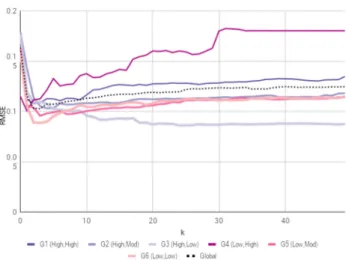
Fig. 17 RMSE’s for pruned neighbourhood-augmented predictions for six participant groups in the mHealth Dataset: Neighbourhoods restricted to groups of participants of similar (Distress=< L/H >, Loudness=<L/M/H>)

low loudness and high distress values in agreement with [9].

The low distress, high loudness group is the smaller of the two, with only 35 participants. It is also seen that while Hiller

& Goebel found about a third of tinnitus patients to be discordant, only about 16% of the participants in the mHealth dataset showed this peculiarity. While this could be a short- coming of the workflow design, it is also possible that the mHealth application is more accessible to tinnitus sufferers who did not go to the hospital ([9] refers to hospital data)

Figure 17 shows the predictions in Dp achieved after segmenting the patients on loudness+distress in Do. Two conclusions, in particular, can be drawn from the results. It can be seen that in four of the six groups, expert knowledge guided intuition contributed to improving prediction quality. In addition, among the groups of patients described in Hiller & Goebel [9] as discrepant in their loudness-distress measurements, one of the corresponding discrepant participant groups (high distress, low loudness) is improved to the greatest extent by the neighbourhood pruning process in the mHealth dataset. In contrast, the predictability in Group4 (low distress, high loudness) is the lowest. This suggests that of the two possible ways in which a patient could be

‘discrepant’, the ones that are distressed to a high degree even with a relatively lower loudness levels are somehow more similar to each other than those of the opposite group (low distress in spite of high loudness). In other words, it could be that participants who find ways do deal with their symptom find their own different ways to deal with it, while those that are easily distressed are more psychologically alike. The RMSE of the global model on Figure 17 indicates that the improvements on some groups are cancelled out by the low predictability on Group 4. Hence the refinement into segmentsisnecessary in order to improve performance.

Indeed, the idea of eliminating false neighbours does have a small positive impact on predictive performance, with four of the six groups showing small improvements in predictive performance compared to the global model that does not exclude neighbours. Since the neighbourhood computations are already (non-randomly) restricted to be within group, we do not compare these results against rNN.

5 Summary and future work

The goal of the study was to investigate whether ak-nearest neighbours constructed on a feature space outside the prediction space of an entity can guide a labelling process for future observations of an entity. Towards this end, we proposed ak-nearest-neighbour method that can work on a static attribute space Do, and transfer the knowledge about entity similarities to label future instances of the entity in dynamic domain Dp. The efficacy of the proposed method is evaluated against a baseline which challenges the assumption that Doyields ‘transferable information’ (by choosingkRandom Entities).

Two methods of combining information from the related entities were observed, and it was seen that a data-augmented method had the best performance. However, more work is needed on a wider range of datasets, before a general conclusion can be reached regarding the selection of the augmentation type with respect to dataset characteristics. It is also to be noted that this early exploratory work only considers the case of linear regression models, and the performance of more complex models such as polynomial regression or ARIMA may be affected to different extents by data augmentation (for example, the fact that data augmentation forcefully aligns all time series can affect ARIMA models in the case of two out-of-sync time series with repeating patterns). Sur- prisingly, it was found that depending on the dataset and its average tendencies, even choosing random entities can improve the prediction quality. This means that even a random entity transfers some level of knowledge about the dataset-level tendency. In other words, it can be argued that a random entity is able to mitigate the sparsity in the available labels. More work needs to be done to verify whether this is generally true across all datasets, and if yes, whether a heuris- tically discoverablekexists that can be used for entities (new, privacy-protected, etc.) that do not have easily computable neighbourhoods.

In this first study on predicting observation labels in an entity-centric way, we did not consider model adaption.

Albeit our results show that it is possible to make even far- future predictions by using solely an initial seed of labelled observations per entity. In addition, we also see that it is possible to incorporate domain-specific expert information to improve predictions by restricting the kNN computation to

(14)

groups of entities in a way that excludes ‘false neighbours’

as suggested in [19]. The adaption of the model with means of semi-supervised or active learning is our next planned task. For this, we intend to build upon our recent works on semi-supervised sentiment classification [10] and on active learning for sentiment classification with an irregularly available oracle [24], both of which are designed for conventional streams though. Our current approach was not optimised with respect to training time and runtime. We want to investigate the impact of dataset characteristics on training time, and to optimise the cost of retraining and adaption if labels can beacquired through an irregularly available oracle or derived with self-learning. The effects of neighbourhood size on model quality and execution time need also further investigation. In our current experiments, the number of neighbours did not exceed 50, whereupon the error values seemed rather stable. Since the number of entities is much smaller than the number of observations, it is worth investigating whether it would be beneficial to set the neighbourhood size relative to the number of entities in the dataset. Several avenues also remain for possible improvements to the core method. The poor gains in predictive performance from the kNN in the Amazon dataset is also possibly due to a poorly trained word embedding model. The evaluation process for the paragraph embedding can possibly be improved by considering a Jac- card coefficient-like measure for the number of neighbours a product has from the same product subcategory.

Acknowledgements Work of Authors 1 and 2 was partially supported by the German Research Foundation (DFG) within the DFG-project OSCAR Opinion Stream Classification with Ensembles and Active Learners. The last two authors are the project’s principal investigators.

References

1. Al-qahtani, F.H.: Multivariate k-Nearest Neighbour Regression for Time Series data—a novel Algorithm for Forecasting UK Electric- ity Demand Multivariate KNN Regression for Time Series. Neural Networks (IJCNN), The 2013 International Joint Conference on pp 228–235 (2013)

2. Ban, T., Zhang, R., Pang, S., Sarrafzadeh, A., Inoue, D.: Referen- tial kNN regression for financial time series forecasting. In: Lee, M., Hirose, A., Hou, Z.G., Kil, R.M. (eds.) Neural Information Processing, pp. 601–608. Springer, Heidelberg (2013)

3. Beyer, C., Niemann, U., Unnikrishnan, V., Ntoutsi, E., Spiliopoulou, M.: Predicting document polarities on a stream without reading their contents. In: Proceedings of the Symposium on Applied Computing (SAC) (2018)

4. Che, Z., Purushotham, S., Cho, K., Sontag, D., Liu, Y.: Recurrent neural networks for multivariate time series with missing values.

Sci. Reports8(1), 6085 (2018)

5. Clarke, R.N.: SICs as Delineators of Economic Markets. J.

Bus. 62(1), 17–31, (1989) https://ideas.repec.org/a/ucp/jnlbus/

v62y1989i1p17-31.html. Accessed 1 Feb 2018

6. Ditzler, G., Roveri, M., Alippi, C., Polikar, R.: Learning in nonstationary environments: a survey. IEEE Comput. Intell. Mag.10(4), 12–25 (2015)

7. Dyer, K.B., Capo, R., Polikar, R.: Compose: A semisupervised learning framework for initially labeled nonstationary streaming data. IEEE Trans. Neural Netw. Learn. Syst.25(1), 12–26 (2014) 8. Hartmann, C., Ressel, F., Hahmann, M., Habich, D., Lehner, W.:

Csar: the cross-sectional autoregression model for short and long- range forecasting. Int. J. Data Sci. Anal. (2019).https://doi.org/10.

1007/s41060-018-00169-7

9. Hiller, W., Goebel, G.: When tinnitus loudness and annoyance are discrepant: audiological characteristics and psychological profile.

Audiol. Neurotol.12(6), 391–400 (2007)

10. Iosifidis, V., Ntoutsi, E.: Large scale sentiment learning with limited labels. In: Proceedings of the 23rd ACM SIGKDD International Conference on Knowledge Discovery and Data Mining, ACM, pp 1823–1832 (2017)

11. Keogh, E.J., Pazzani, M.J.: Scaling up dynamic time warping for datamining applications. In: Proceedings of the Sixth ACM SIGKDD International Conference on Knowledge Discovery and Data Mining, ACM, pp 285–289 (2000)

12. Kia, A.N., Haratizadeh, S., Shouraki, S.B.: A hybrid supervised semi-supervised graph-based model to predict one-day ahead movement of global stock markets and commodity prices. Expert Syst. Appl.105, 159–173 (2018)

13. Krawczyk, B., Minku, L.L., Gama, J., Stefanowski, J., Wo´zniak, M.: Ensemble learning for data stream analysis: a survey. Inf.

Fusion37, 132–156 (2017)

14. Krempl, G., Žliobaite, I., Brzezi´nski, D., Hüllermeier, E., Last, M., Lemaire, V., Noack, T., Shaker, A., Sievi, S., Spiliopoulou, M., et al.: Open challenges for data stream mining research. ACM SIGKDD Explorations Newslett.16(1), 1–10 (2014)

15. Längkvist, M., Karlsson, L., Loutfi, A.: A review of unsupervised feature learning and deep learning for time-series modeling. Pattern Recogn. Lett.42, 11–24 (2014)

16. Le, Q., Mikolov, T.: Distributed representations of sentences and documents. In: International Conference on Machine Learning, pp 1188–1196 (2014)

17. Lora, A.T., Santos, J.R., Santos, J.R., Ramos, J.L.M., Expósito, A.G.: Electricity market price forecasting: Neural networks versus weighted-distance k nearest neighbours. In: International Confer- ence on Database and Expert Systems Applications, Springer, pp 321–330 (2002)

18. Lora, A.T., Santos, J.M.R., Riquelme, J.C., Expósito, A.G., Ramos, J.L.M.: Time-series prediction: Application to the short-term electric energy demand. Current Topics in Artificial Intelligence pp 577–586 (2004)

19. Lora, A.T., Santos, J.M.R., Exposito, A.G., Ramos, J.L.M., San- tos, J.C.R.: Electricity market price forecasting based on weighted nearest neighbors techniques. IEEE Trans. Power Syst. 22(3), 1294–1301 (2007)

20. McAuley, J., Yang, A.: Addressing complex and subjective product-related queries with customer reviews. In: Proceedings of the 25th International Conference on World Wide Web, Inter- national World Wide Web Conferences Steering Committee, pp 625–635 (2016)

21. Polson, N.G., Sokolov, V.O.: Deep learning for short-term traffic flow prediction. Transportation Research Part C: Emerging Tech- nologies79, (2017)

22. Pryss, R., Probst, T., Schlee, W., Schobel, J., Langguth, B., Neff, P., Spiliopoulou, M., Reichert, M.: Prospective crowdsensing versus retrospective ratings of tinnitus variability and tinnitus-stress associations based on the trackyourtinnitus mobile platform. Int. J.

Data Sci. Anal. (2018).https://doi.org/10.1007/s41060-018-0111- 4

23. ˇReh˚uˇrek, R., Sojka, P.: Software Framework for Topic Modelling with Large Corpora. In: Proceedings of the LREC 2010 Workshop on New Challenges for NLP Frameworks, ELRA, Valletta, Malta, pp 45–50 (2010)