Dielectric Properties and Cooperative Dynamics of Protic and Aprotic Room-Temperature Ionic Liquids
Dissertation zur Erlangung des
Doktorgrades der Naturwissenschaften (Dr. rer. nat.)
der Naturwissenschaftlichen Fakultät IV Chemie und Pharmazie
der Universität Regensburg
vorgelegt von Thomas Sonnleitner
aus Regensburg
Regensburg 2013
Promotionsgesuch eingereicht am: 10.12.2013 Tag des Kolloquiums: 31.01.2014
Die Arbeit wurde angeleitet von: Apl. Prof. Dr. R. Buchner Prüfungsausschuss: Apl. Prof. Dr. R. Buchner
Prof. Dr. W. Kunz Prof. Dr. A. Pfitzner
Prof. Dr. J. Daub (Vorsitzender)
für
meine Eltern meine Schwester
und Susi
Vorwort
Diese Doktorarbeit entstand in der Zeit von Oktober 2010 bis Dezember 2013 am Insti- tut für Physikalische und Theoretische Chemie der naturwissenschaftlichen Fakultät IV – Chemie und Pharmazie – der Universität Regensburg.
An erster Stelle möchte ich mich bei Herrn Apl. Prof. Dr. Richard Buchner für die Erteilung des Themas bedanken. Sein Interesse am Fortschritt der Arbeit, die stete Bereitschaft zur fachlichen Diskussion sowie seine wertvollen Ratschläge haben wesentlich zum Gelingen dieser Arbeit beigetragen. Neben den zahlreichen Dienstbesprechungen danke ich ihm besonders für die Ermöglichung mehrerer Konferenzteilnahmen und Forschungsaufenthalte.
Des Weiteren gilt mein Dank dem Leiter des Lehrstuhls, Herrn Prof. Dr. W. Kunz für die Bereitstellung der Laboratorien und Verbrauchsmaterialien.
Der deutschen Forschungsgemeinschaft (DFG) sei für die Finanzierung sowie die Bereitstel- lung der Mittel zur Durchführung des Projektes im Rahmen des Schwerpunktprogramms 1191 gedankt.
Ferner möchte ich mich bei folgenden Kooperationspartnern bedanken, ohne deren Unter- stützung wesentliche Teile dieser Arbeit nicht möglich gewesen wären:
• Herrn Prof. Dr. Glenn Hefter (Murdoch University, Western Australia) danke ich für seine stete Diskussionsbereitschaft und die große Unterstützung hinsichtlich des in Kapitel 3.1 präsentierten Materials. Ihm und seiner Frau Miriam sei ebenfalls für die ein oder andere Dienstbesprechung gedankt.
• Herrn Prof. Dr. Klaas Wynne und Dr. David Turton (Glasgow University, Glasgow, UK) danke ich ganz besonders für zwei Forschungsaufenthalte in Glasgow, welche für mich nicht nur fachlich, sondern auch persönlich von unschätzbarem Wert waren.
Besonders danken möchte ich Dr. David Turton für die intensive Zusammenarbeit auf dem Gebiet der Ferninfrarot- und Optischen Kerr-Effekt Spektroskopie, wodurch wesentliche Teile dieser Arbeit entstanden sind.
• Herrn Dr. M. Walther (Albert-Ludwigs-Universität, Freiburg) sowie seinen Mitar- beitern, Dipl. Phys. Alex Ortner und Dipl. Phys. Stefan Waselikowski danke ich im Besonderen für die Durchführung der THz-TDS-Messungen zahlreicher Proben.
i
ii
• Herrn Dr. Johannes Hunger (Max-Planck Institut, Mainz, Germany) danke ich außeror- dentlich für die fruchtbare Zusammenarbeit und die vielen wertvollen Diskussionen auf dem Gebiet der Dielektrischen Relaxationsspektroskopie.
• Herrn Prof. Dr. O. Steinhauser und Dr. C. Schröder (University of Vienna, Austria) möchte ich für die Zusammenarbeit und Diskussionen auf zahlreichen Konferenzen danken.
• Frau M. Sc. Viktoriya Nikitina danke ich für die gute Zusammenarbeit bezüglich des in Kapitel 5 präsentierten Materials.
• Herrn Prof. Dr. Y. Umebayashi und M. Sc. Hiroyuki Doi (Niigata University, Niigata, Japan) danke ich für die angenehme Zusammenarbeit und die zur Verfügungstellung einiger Messungen des in Kapitel 3.2 präsentierten Materials. Besonders möchte ich mich bei M. Sc. Hiroyuki Doi für die herausragende Betreuung bei der ICSC Konferenz in Kyoto bedanken. In diesem Zusammenhang gilt mein Dank auch Herrn Dr. M. Kanakubo (National Institute of Advanced Industrial Science and Technology, Sendai, Japan), welcher die Teilnahme ermöglicht hat.
Bei allen Mitarbeitern und Kollegen des Lehrstuhls möchte ich mich für die freundschaftliche Atmosphäre und stete Hilfsbereitschaft bedanken. Dabei richtet sich mein besonderer Dank an die ehemaligen Mitarbeiter des AK Buchner, Herrn Dr. Johannes Hunger, Herrn Dr. Alexander Stoppa, Herrn Dr. Hafiz Rahman und Frau Dr. Saadia Shaukat, für die freundschaftliche Aufnahme in die Arbeitsgruppe, die Einweisung in die Messinstrumente und ihre zahlreichen Tipps, welche entscheidend zum Gelingen dieser Arbeit beigetra- gen haben. Des Weiteren gilt mein besonderer Dank Herrn Dr. Andreas Eiberweiser für die langjährige Zusammenarbeit. Die freundschaftliche Arbeitsatmosphäre und seine stete Diskussionsbereitschaft über fachliche und nicht-fachliche Themen waren für mich eine Be- reicherung. Ebenso bedanke ich mich ganz herzlich bei meinem aktuellen Kollegen M. Sc.
Andreas Nazet, welcher mir besonders mit seinen fundierten Programmierkenntnissen jed- erzeit mit Rat und Tat zur Seite stand.
Ganz besonders möchte ich auch meiner Familie und meiner Freundin Susi danken, welche stets mit großem Interesse meinen Werdegang verfolgt haben und mich jederzeit unterstützt haben.
Für die mentale Unterstützung am Arbeitsplatz möchte ich mich herzlich bei meiner Mensa- Essensgruppe und allen Teilnehmern der Kaffeerunde bedanken, welche täglich für einen angenehmen Ausgleich gesorgt haben.
Nicht zuletzt möchte ich allen Mitarbeitern der Werkstätten für die schnelle und gewis- senhafte Erledigung der Aufträge meinen Dank aussprechen.
Contents
Introduction 1
1 Theoretical Background 5
1.1 Fundamentals of dielectric relaxation . . . 5
1.1.1 Polarization . . . 5
1.1.2 Response function . . . 6
1.1.3 Optical constants . . . 8
1.2 Empirical models . . . 11
1.2.1 Relaxation processes . . . 11
1.2.2 Resonance processes . . . 14
1.3 Microscopic models of dielectric relaxation . . . 15
1.3.1 Onsager equation . . . 15
1.3.2 Kirkwood-Fröhlich equation . . . 16
1.3.3 Cavell-equation . . . 16
1.3.4 Debye model of rotational diffusion . . . 17
1.3.5 Model of jump relaxation . . . 19
1.3.6 Microscopic and macroscopic relaxation times . . . 19
1.4 Temperature dependence of relaxation times . . . 20
1.4.1 Arrhenius equation . . . 20
1.4.2 Eyring equation . . . 20
1.4.3 Vogel-Fulcher-Tammann equation . . . 21
2 Experimental 23 2.1 Materials and Sample Handling . . . 23
2.2 Measurement of Dielectric Properties . . . 25
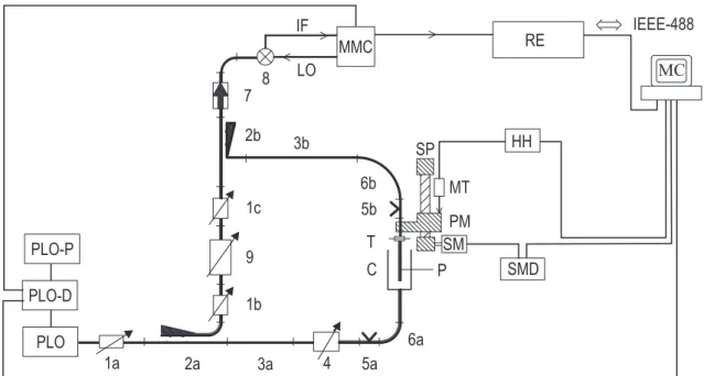
2.2.1 Interferometry . . . 25
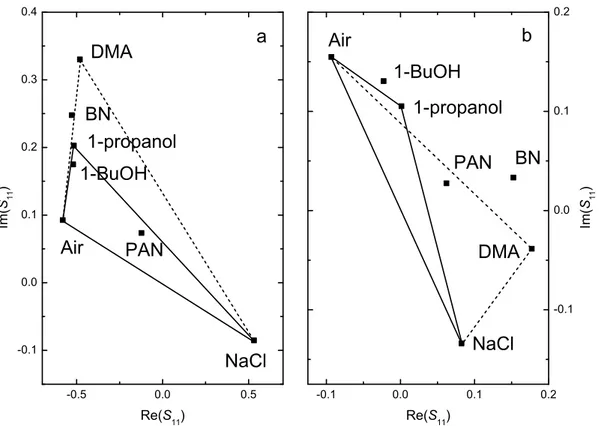
2.2.2 Vector Network Analysis . . . 28
2.2.3 Time-domain THz-pulse Spectroscopy . . . 33
2.2.4 Far-infrared Spectroscopy . . . 36
2.3 Optical Kerr-Effect Spectroscopy . . . 37
2.4 Data processing . . . 40
2.5 Auxiliary Measurements . . . 41
2.5.1 Density . . . 41
2.5.2 Viscosity . . . 42
2.5.3 Electrical Conductivity . . . 42
2.5.4 Refractive indices . . . 42
2.5.5 Quantum Mechanical Calculations . . . 43 iii
iv CONTENTS
3 Neat Protic Ionic Liquids 45
3.1 Ethyl- and Propylammonium Nitrates . . . 45
3.1.1 Introduction . . . 45
3.1.2 Data acquisition and processing . . . 46
3.1.3 Results . . . 47
3.1.4 Discussion of “slow” dynamics . . . 59
3.1.5 Discussion of “fast” dynamics . . . 63
3.1.6 Conclusions . . . 70
3.2 1-Methylimidazolium-based Protic ILs . . . 73
3.2.1 Introduction . . . 73
3.2.2 Data acquisition and processing . . . 74
3.2.3 Results . . . 74
3.2.4 Discussion . . . 79
3.2.5 Conclusions . . . 88
4 Neat Aprotic Ionic Liquids 91 4.1 Introduction . . . 91
4.2 Data acquisition and processing . . . 92
4.3 Results . . . 93
4.3.1 Densities, Viscosities and Conductivities . . . 93
4.3.2 Dielectric and Optical Kerr-Effect Spectroscopy . . . 94
4.4 Discussion . . . 110
4.4.1 Static permittivities . . . 110
4.4.2 Low-Frequency processes . . . 111
4.4.3 High-Frequency processes . . . 123
4.5 Conclusions . . . 125
5 Binary mixture of EAN + Acetonitrile 127 5.1 Introduction . . . 127
5.2 Experimental . . . 128
5.2.1 Materials and auxiliary measurements . . . 128
5.2.2 Dielectric Spectroscopy . . . 129
5.3 Results and Discussion . . . 130
5.3.1 Choice of fit model . . . 130
5.3.2 Higher frequency mode . . . 133
5.3.3 Lower frequency mode . . . 136
5.4 Concluding Remarks . . . 141
Summary and Conclusion 143 Appendix 149 A.1 Physical Properties of neat Aprotic ILs . . . 149
A.1.1 Densities, Viscosities and Conductivities . . . 149
A.1.2 Refractive indices and polarizabilities . . . 156
A.2 DRSFit Manual . . . 159
Bibliography 171
Constants and symbols
Constants
Electric field constant εo = 8.854187816·10−12C2(Jm)−1 Avogadro’s constant NA = 6.0221367·1023mol−1
Speed of light c = 2.99792458·108m s−1 Boltzmann’s constant kB = 1.380658·10−23J K−1 Permittivity of vacuum µ0 = 4π·10−7(Js)2(C2m)−1 Planck’s constant h = 6.6260755·10−34Js
Symbols
E⃗ electric field strength (V m−1) P⃗ polarization (C m−2)
n refractive index εˆ complex dielectric permittivity χ electric susceptibility ε′ real part of εˆ
ω angular frequency (s−1) ε′′ imaginary part ofεˆ τ relaxation time (s) ε∞ limν→∞(ε′)
η viscosity (Pa s) εs limν→0(ε′)
T temperature (K) µ dipole moment (C m)
t time (s) ν frequency (Hz)
c molarity (mol dm−3) λ wavelength (m) κ conductivity (S m−1) ρ density (kg m−3)
vi CONTENTS
Acronyms
AN acetonitrile AIL aprotic ionic liquid
BN benzonitrile 1-BuOH 1-butanol
CC Cole-Col CD Cole-Davidson
CIP contact ion-pair D Debye
DCA dicyanamide DHO damped harmonic oscillator
DMA N,N-dimethylacetamide DMF N,N-dimethylformamide DR(S) dielectric relaxation (spec-
troscopy) EAN ethylammonium nitrate
FIR far-infrared HN Havriliak-Negami
G antisymmetrized Gaussian IFM interferometer
IL ionic liquid IR infrared
MD molecular dynamics C1Im 1-methylimidazole
NMR nuclear magnetic resonance OKE optical Kerr-effect
TPX polymethylpentene PAN propylammonium nitrate
PIL protic ionic liquid PRT platinum resistance thermome- ter
PTFE polytetrafluoroethylene RTIL room temperature ionic liquid SED Stokes-Einstein-Debye SIP solvent separated ion-pair TDR time-domain reflectometry TFSA bis(trifluoromethanesulfonyl)-
amide THz-TDS terahertz time-domain spec-
troscopy vdW van der Waals
VFT Vogel-Fulcher-Tammann VNA vector network analyzer
Introduction
For more than two decades ionic liquids (ILs) have been attracting increasing attention due to their unique combination of properties.1–4 Entirely consisting of ionic species, ILs represent a sub-class of compounds, which are traditionally known as molten salts. With the onset of intensive IL research in the late 1990’s, the term “ionic liquid” has been established to denote those salts with melting points or glass-transition temperatures be- low 100◦C.1,5 Possibly the first discovered salt that meets this condition was ethanolam- monium nitrate and was reported as early as in 1888 by Gabriel6 with a melting point of ∼ 52− 55◦C.7 A separate niche of ILs are those being liquid at ambient tempera- tures, therefore commonly referred to as room-temperature ionic liquids (RTILs). In 1914, Walden reported the physical properties of ethylammonium nitrate (EAN, melting point:
14◦C),8 which today is widely acknowledged as the advent of the field of ILs but has not received much attention at that time. A “new class of room-temperature ionic liquids”9 based on dialkylimidazolium chloroaluminates has been reported in 1982 followed, ten years later, by the discovery of apparently “air and water stable 1-ethyl-3-methylimidazolium- based ionic liquids”10formed with weakly coordinating anions such as hexafluorophosphate PF−6 and tetrafluoroborate, BF−4, representing another benchmark in IL research. Because of the later observed hydrolysis of PF−6,11 which is accompanied by the undesirable re- lease of hydrofluoric acid, the development of ILs based on more hydrophobic anions such as bis(trifluoromethanesulfonyl)amide (TFSA−) received increasing interest, which, apart from their lower hygroscopicity, have attracted particular attention for potential applica- tions in electrochemical devices, due to their enhanced electrochemical windows.12,13 Since that time, the interest in ILs has continuously grown, which has manifested itself not only in a nearly exponential increase of publications13 but also in scientific programs such as the “DFG-SPP 1191 priority program: ionic liquids” started in 2006 specifically dedicated to improve “understanding of the special nature of ionic liquids through fundamental re- search”.14 Nowadays, ILs are known to offer important advantages in electrochemistry,15 organic synthesis and catalysis5,16,17 because of their negligible vapor pressure,18high ther- mal and electrochemical stability,19,20 and solubilizing capabilities.21–23 Furthermore, due to the almost unlimited possible combinations of cations and anions, the properties of ILs can be fine-tuned selectively for specific applications,13,24,25 which brought them the name of “designer solvents”. The issue of ILs’ toxicity has been controversially discussed over many years. Recently, toxicity and biodegradability studies received increasing attention eventually leading to the consensus that the commonly accepted notion of the low toxicity of ILs is incorrect.23,26,27
Generally, the wide field of ILs can be subdivided into two major sub-groups: protic ILs 1
2 INTRODUCTION
(PILs) and aprotic ILs (AILs). In contrast to AILs, PILs, whose most prominent repre- sentative is EAN,7,28 are formed by the combination of a Brønsted acid and a Brønsted base through proton transfer reaction. This leads to their key characteristics, which is the ability to form hydrogen-bonded networks.
At the beginning of this thesis in 2010, the most intensively studied ILs among the group of AILs, were those based on 1-alkyl-3-methylimidazolium cations.2,17,29,30 Of particular rele- vance for the present work is the progress in understandingstructural anddynamical prop- erties of ILs. Also in this regard, early investigations using spectroscopic techniques29,31–39 and MD simulations40–45 have mainly focused on neat 1-alkyl-3-methylimidazolium ILs and their binary mixtures with molecular solvents.46–51 This also applies to investiga- tions of the dielectric properties of RTILs, where Weingärtner et al.30,52–55 and Buchner et al.46,47,49,56–58 have certainly published the most important contributions. With the begin- ning of the present work, two comprehensive theses59,60 have been finished in our group, primarily dealing with dynamics of binary mixtures of ILs with polar molecular solvents but also with those of a representative set of neat 1-alkyl-3-methylimidazolium ILs.
As a consequence, PILs and AILs constituted of other cations such as pyridinium, pyrroli- dinium, phosphonium or sulfonium have been out of the major focus of IL research, except for some recent investigations that include studies using NMR-relaxation,61–63 far-infrared (FIR) spectroscopy,64–66 optical heterodyne-detected Kerr-effect (OKE) spectroscopy,67–69 time-resolved fluorescence spectroscopy,70 quasi-elastic neutron scattering (QENS)71 and MD simulations.72–74In particular, dielectric studies are very scarce up to now. Apart from few works,46,52,54,75 which, however, were limited in their investigated frequency and/or temperature range, dielectric properties and intermolecular dynamics of PILs and non- imidazolium AILs have been almost unexplored.
The static dielectric permittivity, εs, represents a fundamental quantity for characterizing the polarity of a solvent. The question of “how polar are ionic liquids?”76 has been contro- versially discussed for a long time, mainly because inappropriate methods have been used for the determination of εs. Eventually, this dispute was settled by means of dielectric relaxation spectroscopy (DRS),52,58,76 which represents the only technique available for di- rectly determining εs of conducting samples. Apart from that, dielectric spectra provide valuable insight into dynamical properties of liquids within the MHz to THz frequency region.57,77 In particular, comparative studies using other spectroscopic techniques such as OKE spectroscopy have shown to be powerful tools for investigating the dynamics of liquids as complex as RTILs.36 Although considerable effort has been made, still no sat- isfactory picture of the molecular-level dynamics of RTILs in general and of PILs and non-imidazolium AILs in particular has emerged up to date.
Aims of this study
The overall aim of this thesis is the investigation of the dielectric properties and intermolec- ular dynamics of RTILs. DRS is used as the main technique and is complemented by OKE spectroscopy, for most of the studied neat ILs. Additionally, physicochemical properties such as density, viscosity and electrical conductivity are reported. In general the present
INTRODUCTION 3
work can be subdivided into three parts:
First, dielectric properties and dynamics of representative neat PILs are investigated (Chapter 3). The archetypal PILs EAN and propylammonium nitrate (PAN) are stud- ied over the exceptional wide frequency range 0.2 ≤ ν/GHz ≤ 10 000 by means of DRS and OKE spectroscopy (Section 3.1). Both EAN and PAN exhibit rather simple chemical structures and thus can be viewed as model PILs. EAN has been studied by DRS52, THz spectroscopy75 and FIR spectroscopy,64,65 however, limitations in either frequency or tem- perature range prevented a detailed analysis of the intermolecular dynamics. Therefore, in the present work, measurements of DR and OKE spectra over a temperature range of 60 K supplemented by DR and OKE spectra of partially deuterated (d3-)EAN at 25◦C enables extensive characterization of the dynamics of EAN and PAN ranging from MHz to THz frequencies. The results so obtained improve and partially correct hitherto accepted interpretations.
Furthermore, a set of 1-methylimidazolium PILs is studied in collaboration with a Japanese research group (Prof. Dr. Umebayashi, Niigata University, Niigata, Japan) by DRS in the limited frequency range 0.2 ≤ ν/GHz ≤ 89 (Section 3.2). In particular, the influ- ence of proton transfer and temperature on the dynamics of the equimolar mixture of 1-methylimidazole (C1Im) with acetic acid (HOAc) will be investigated. This system has been studied by calorimetric titration78 and Raman spectroscopy,79however, controversial results with respect to the degree of proton transfer have been obtained. In this regard, an attempt is made to provide new insights by quantitative analysis of the present DR spectra.
Second, broadband DR and OKE spectra (0.2≤ν/GHz≤10 000) of a set of four represen- tative neat non-imidazolium AILs are recorded in the temperature range of5≤ϑ/◦C≤65 (Chapter 4). These ILs were chosen, because of their commercial availability at a sufficient purity, thus serving as model non-imidazolium AILs. Based on the TFSA− and the di- cyanamide (DCA−) anion 1-alkyl-3-methylimidazolium cations are replaced by pyridinium, pyrrolidinium and sulfonium cations to scrutinize the effect of cation variation on DR and OKE spectra. Particular focus was on the diffusional dynamics taking place from MHz to GHz frequencies associated with fluctuations of mesoscale clusters and the cooperative relaxation of anions and cations. In this regard, temperature and viscosity dependence of DR and OKE relaxation times provide valuable insights into the molecular-level dynamics of RTILs and how these may determine macroscopic transport properties such as viscosity and electrical conductivity, which is of exceptional importance for scientific and industrial applications.
Third, the binary mixture of EAN and acetonitrile (AN) is investigated as a model system of a PIL+molecular solvent mixture (Chapter 5). Therefore, DR spectra are recorded in the frequency range 0.2 ≤ ν/GHz ≤ 89 at 25◦C over the entire composition range. As mentioned above, most publications dealing with the dynamics of binary mixtures of ILs with molecular solvents have focused on salts with 1-alkyl-3-methylimidazolium cations but only little is known about PIL-containing systems, up to now.80,81 In practical appli- cations ILs are generally mixed with other compounds. Thus, it is essential to understand
4 INTRODUCTION
their structure and dynamics. In this regard, the transition from IL-like dynamics to that of conventional electrolyte solutions is of particular interest, which will be addressed in the present work. Additionally, the formation of ion pairs, which is a common feature of conventional electrolyte solutions at low salt concentrations77,82 will be quantitatively in- vestigated in the present EAN+AN mixtures. Furthermore, information on solvent/solute dynamics will be extracted providing insight into intermolecular interactions and their de- pendence on composition.
To analyze DR and OKE spectra recorded over such a broad frequency range (0.2 ≤ ν/GHz ≤ 10 000), a new fitting program was required (Appendix A.2). In close col- laboration with Dr. D. A. Turton (Glasgow University, Glasgow, UK), who developed a rudimentary version, a fitting routine (DRSFit) based on the commercially available IGOR software (Wavemetrics, V.6.31) has been established in our group. The ability of fitting DR as well as OKE spectra and implementation of new empirical model functions rank among the key advantages of this program.
Chapter 1
Theoretical Background
1.1 Fundamentals of dielectric relaxation
1.1.1 Polarization
Electrodynamic theory is based on Maxwell’s equations, which form a set of four linear partial differential equations that are capable to describe all classical phenomena of elec- tromagnetic radiation.83,84 Within this theory the response of a material to an applied low-intensity electric field, E, is described by the phenomenon of polarization,⃗ P⃗, which is defined as the macroscopic dipole moment of the sample per unit volume. It results from an effective charge separation in the medium and is proportional toE⃗ by
P⃗ =χε0E⃗ (1.1)
in case of a linear and isotropic medium. The proportionality factor χ(= εs−1) is the electric susceptibility andε0 and εs are the permittivity of free-space and the relative per- mittivity of the medium, respectively.85 Although P⃗ is defined as a macroscopic quantity, it can be also interpreted on a microscopic level by splitting it up into two contributions
P⃗ =P⃗µ+P⃗α (1.2)
where P⃗µ and P⃗α are the dipolar (orientational) and induced polarization, respectively.
Within the continuum approach, P⃗µ is explained by the alignment of permanent dipoles embedded in a continuum of permittivity, εs, along the applied electric field. Its estab- lishment takes place on the picosecond to nanosecond time scale, which corresponds to frequencies in the microwave region. It is associated with rotations of the dipole vectors and is given as
P⃗µ=∑
j
ρj⟨µj⟩ (1.3)
where ρj is the dipole density and ⟨µj⟩ the ensemble average of the permanent dipole vector.86 The complete alignment, however, is counteracted by the thermal motion of the molecules, which makes P⃗ strongly dependent on the temperature.
The induced polarization,P⃗α, can be understood as an intramolecular translational effect, 5
6 CHAPTER 1. THEORETICAL BACKGROUND
that can be separated into two contributions: the atomic polarization that results from the displacement of the nuclei of a molecule relative to each other (vibrations) and the electronic polarization that is caused by the displacement of the electrons relative to the positive charges (nuclei).86 It is expressed as
P⃗α =∑
j
ρjαj(E⃗int)j (1.4)
whereαj is the polarizability and(E⃗int)j the internal field (cavity field) of thejth particle, which is defined as the total electric field acting on a particle minus the field generated by the particle itself.86
The fact that P⃗µ and P⃗α take place on sufficiently different time scales permits both to be considered as linearly independent. By introduction of ε∞, P⃗µ and P⃗α can be written as
P⃗µ= (εs−ε∞)ε0E⃗ (1.5)
P⃗α = (ε∞−1)ε0E⃗ (1.6)
whereε∞ is the permittivity at frequencies at which the orientational polarization is com- pletely decayed, but the induced polarization still remained unchanged (typically at a few THz).87
1.1.2 Response function
In case of rapidly changing electric fields, the polarization is no longer directly proportional to the applied field strength as stated by Eq. 1.1, because P⃗ then depends on the values of E⃗ at all moments before the time t at which P⃗ is considered.86 Thus, the generalized relation between the polarization and an arbitrary time-dependent electric field is given by
P⃗(t) =ε0χ
∫0
−∞
fP(t−t′)E(t⃗ ′)dt′ (1.7) wherefP(t−t′)is the pulse-response function of the polarization, which in turn is defined as the negative time-derivative of the step response function,FP(t−t′),86
fP(t−t′) =−∂FP(t−t′)
∂(t−t′) normalized by
∫∞
0
fP(t′)dt′ = 1. (1.8)
In a time-domain experiment, a polarization P⃗ in a dielectric medium, which is generated by application of an external field, E, decreases from⃗ P⃗(0) to P⃗(∞) = 0 when the field is switched off at t= 0. It is then assumed that on the time scale of a dielectric experiment, P⃗α breaks down “instantaneously”, whereas P⃗µ decays monotonically to its final value of
1.1. FUNDAMENTALS OF DIELECTRIC RELAXATION 7 P⃗µ(∞) = 0.87 This can be mathematically expressed as
P⃗µ(t) = P⃗µ(0)·FP(t) with FP(0) = 1 and FP(∞) = 0 (1.9) where the step-response function, FP(t), is defined as the time-correlation function of the orientational polarization and is given as88
FP(t) = ⟨P⃗µ(0)·P⃗µ(t)⟩
⟨P⃗µ(0)·P⃗µ(0)⟩ (1.10) In case of a harmonically oscillating field, E(t) =⃗ E⃗0exp(iωt), the frequency-dependent orientational polarization is then written as
P⃗µ(ω, t) =ε0(εs−ε∞)E(t)⃗
∫∞
0
exp(iωt′)fP(t′)dt′ (1.11)
with ∫∞
0
exp(iωt′)fP(t′)dt′ =Liω[fP(t′)] (1.12) where Liω[fP(t′)] is the Laplace transformation of the pulse-response function.
With this relation, the permittivity can be expressed as a complex quantity, which is defined as89
ˆ
ε(ω) =ε′(ω)−iε′′(ω) =ε∞+ (εs−ε∞)· Liω[fP(t′)] =ε∞+ (εs−ε∞)·F˜P(ω) (1.13) where the relaxation function, F˜P(ω), is the frequency analogue to the step-response func- tion, FP(t).
In Eq. 1.13 the real part, ε′(ω) of ε(ω)ˆ represents the relative permittivity and is a mea- sure of the polarization of the medium at a certain angular frequency, ω = 2πν, whereas the imaginary part, ε′′(ω), known as the dielectric loss or absorption describes the energy dissipation in the system. The phase shift between the electric field and the polarization is expressed by the loss angle, tanδ =ε′′(ω)/ε′(ω), which can be interpreted as a measure of the deviation of the system from equilibrium.90
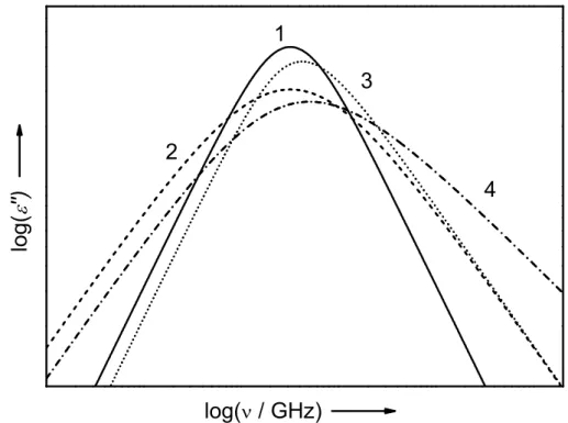
In Figure 1.1 a schematic broadband dielectric spectrum is shown. Apart from possible interfacial polarization effects, which may contribute to ε(ν)ˆ for heterogeneous systems at MHz frequencies,86,91the main contribution in the microwave region arises from rotational motions of molecules with permanent dipole moment. As the frequency, ν(= ω/2π), in- creases dispersion of ε′(ν), accompanied by a simultaneously emerging absorption band in ε′′(ν), is observed. This is a consequence of the inability of the molecules to follow the applied electric field. In addition to molecular rotations, “cage rattling” motions, in- termolecular vibrations (e.g. hydrogen-bonding), and librations, which are described as hindered rotations or tumbling motions of the dipoles confined in intermolecular poten- tials, contribute to ε(ν)ˆ at frequencies up to several THz.86 Due to the coupling of dipoles to their environment, the band-shape of all these processes, in particular of relaxations, is
8 CHAPTER 1. THEORETICAL BACKGROUND
Figure 1.1: Schematic spectrum of the complex permittivity, ε(ν), with real part,ˆ ε′(ν) (black solid line), and imaginary part, ε′′(ν) (gray solid line). Exemplarily, a dielectric relaxation process (microwave region), an intramolecular vibration (infrared region) and an electronic resonance (ultra-violet region) is shown.
rather broad. Along with the entire decay of the orientational polarization, ε′(ν) reaches its high frequency limit, ε∞, and thus marks the transition to intramolecular processes, which are associated with the induced polarization, P⃗α, including molecular vibrations (IR region) and electronic excitations (UV/Vis region). The intramolecular nature manifests itself in resonance-type dispersion steps and absorption peaks, which are narrower than those of intermolecular bands.92
1.1.3 Optical constants
As discussed in Section 1.1.1 the interaction of electromagnetic radiation with matter is described by Maxwell’s equation and leads to a polarization, P⃗ (Eq. 1.1), of the dielectric medium, which can be expressed in terms of the complex permittivity, ε(ν)ˆ (Eq. 1.13).
For a plane wave travelling a distance, z, through an isotropic medium, the electric field, E(t, z), is defined by⃗ 86
E(t, z) =⃗ E⃗0exp(iωt)·exp(−ˆγz) (1.14) where ˆγ is the complex propagation coefficient, which is given by93
ˆ
γ =αa+ iβ = [ˆµµ0(iωκˆ−εεˆ 0ω2)]12 (1.15)
1.1. FUNDAMENTALS OF DIELECTRIC RELAXATION 9
with attenuation coefficient, αa, and phase constant, β. Furthermore in Eq. 1.15, µˆ and κˆ are the complex permeability and the complex conductivity, respectively. Both quantities are defined in analogy to εˆby
ˆ
µ(ω) = µ′(ω)−iµ′′(ω) (1.16) ˆ
κ(ω) = κ′(ω)−iκ′′(ω) (1.17) In case of non-magnetic samples (µˆ= 1), as all of the studied liquids in this work, Eq. 1.15 reduces to
ˆ γ = iω
c0
√ ˆ
ε(ω) + κ(ω)ˆ
iωε0 = ik0√
η(ω) = iˆk (1.18)
where k0 = ω√
ε0µ0 = ω/c0 = 2π/λ0 is the propagation constant of free space of a wave with wavelengthλ0 andη(ω)is the generalized complex permittivity of the medium.94 For coaxial lines and free-space methods Eq. 1.18 is valid andγˆ in Eq. 1.14 can be replaced by iˆk (Eq. 1.26). For waveguide instrumentsγˆ has to be modified according to the boundary conditions imposed by the geometry of the waveguide, as will be discussed in Section 2.2.1.94 The generalized complex permittivity,η(ω), which is the experimentally accessibleˆ quantity, is then related to ε(ω)ˆ via
ε′(ω) =η′(ω) + κ′′(ω)
ωε0 (1.19)
ε′′(ω) =η′′(ω)− κ′(ω)
ωε0 (1.20)
These two equations (Eqs. 1.19 and 1.20) reveal thatεˆandκˆcannot be measured indepen- dently. As the theory of Debye and Falkenhagen95predicts a dispersion of the conductivity, this makes a separation of εˆand ˆκ impossible and thus particularly affects the discussion of dielectric parameters of conductive systems. However, the dispersion of κˆ is typically small96 with its known limits limω→0κ′ = κ and limω→0κ′′ = 0 with dc conductivity, κ.
Application of these limits to Eqs. 1.19 & 1.20 lead to
ε′(ω) =η′(ω) (1.21)
ε′′(ω) =η′′(ω)− κ ωε0
(1.22) This implies that for conductive samples, ε(ω)ˆ is obtained from η(ω)ˆ by subtracting the Ohmic loss contribution associated with κ. As a consequence, a potential dispersion of the conductivity is incorporated in ε, thus exacerbating the interpretation of dielectricˆ parameters.
The generalized complex permittivity, η(ω)ˆ is further related to the complex refractive
10 CHAPTER 1. THEORETICAL BACKGROUND
index, n(ω)ˆ via
ˆ
n(ω) = √ ˆ
η(ω) = n(ω)−iξ(ω) (1.23)
wheren is the refractive index that appears in Snell’s law andξ the absorption constant.a The relation of both quantities toη′(ω) and η′′(ω) is given by97
n(ω)2 = 1 2
√η′(ω)2+η′′(ω)2+η′(ω) (1.24)
ξ(ω)2 = 1 2
√η′(ω)2+η′′(ω)2−η′(ω) (1.25)
Following Ref. 9494, insertion of Eqs. 1.18 and 1.23 into Eq. 1.14 yields an expression for travelling waves without boundary conditions
E(t, z) =⃗ E⃗0exp[−ξk0z] exp[i(ωt−nk0z)] =E⃗0exp[−αaz] exp[i(ωt−βz)] (1.26) that holds for free-space methods (Section 2.2.3) and coaxial lines (Section 2.2.2). Com- parison of Eq. 1.26 with Eq. 1.15 then reveals that the attenuation coefficientαa =ξk0 and the phase constant β = nk0 = 2π/λM, with λM as the medium wavelength. Using the definition of the intensity,I(z),
I(z)∝E⃗ ·E⃗∗ (1.27)
where E⃗∗ is the complex conjugate of E, leads directly to the absorption law of Lambert-⃗ Beer98
I(z)
I(0) = e−2αaz := e−αz (1.28)
with α= 2αa defined as the absorption coefficient. Accordingly, permittivity spectra η(ν)ˆ can be converted into absorption spectra α(ν), via the absorption constant ξ defined by Eq. 1.25 and with ω = 2πν by
α(ν) = 4πν
c0 ξ (1.29)
thus forming the basis of the concatenation of far-infrared and dielectric spectra, as de- scribed in Section 2.2.4.
aNote that the latter is commonly labelled ask or κ. However, to avoid confusion with propagation constant and conductivity,ξis used here.
1.2. EMPIRICAL MODELS 11
1.2 Empirical models
bTo describe the spectra recorded in this work (dielectric and OKE spectra), various empiri- cal and semi-empirical model functions are available in literature.86,92Especially broadband spectra ranging from hundreds of MHz to tens of THz are comprised of a superposition of several intermolecular modes. Ideally the spectra can be decomposed into their individ- ual contributions and thus can be modelled by sums of n single relaxation and resonance processes with amplitude, Sj =εj−εj+1, and band shape, Fj(ω),
ˆ
ε(ω) =ε∞+
∑n
j=1
SjFj(ω) (1.30)
At lower frequencies (. 100GHz) the measured intensity is best described by relaxation functions (Section 1.2.1), whereas at higher frequencies (&100GHz) resonance-type band- shapes (Section 1.2.2) are more appropriate. In this section the model functions used in this work are presented.
1.2.1 Relaxation processes
Debye equation
The simplest approach to describe the dielectric spectrum of a liquid is the Debye equa- tion.99 As shown by Pellat100 it is based on the assumption that the decrease of the orientational polarization in the absence of an external electric field follows a time law of first order with a characteristic time constant τ,
∂
∂t
P⃗µ(t) =−1 τ
P⃗µ(t). (1.31)
Solution of this equation yields
P⃗µ(t) = P⃗µ(0) exp (
−t τ
)
(1.32) where the exponential term represents the step-response function according to Eq. 1.10.
Using Eq. 1.8 the pulse response function can be determined, which in turn allows the calculation of the response function, FD(ω) (Eq. 1.13), yielding the Debye equation (D;
curve 1 in Figure 1.2)
FD(ω) = 1
1 + iωτ (1.33)
bNote that although the model functions presented in this section are primarily introduced for describ- ingε(ω), the imaginary part of OKE spectra can be treated equivalently.ˆ
12 CHAPTER 1. THEORETICAL BACKGROUND
Extensions of the Debye equation
Most of the real spectra cannot be solely modelled by a mono-exponential relaxation using the Debye equation. In these cases band-shape functions that describe a distribution of relaxation times are more desirable. However, from such an approach no closed analytical form can be obtained in the frequency domain. Alternatively, the Debye model can be extended by using empirical parameters in order to symmetrically and/or asymmetrically broaden the dispersion and absorption curve of Eq. 1.33. The broadening is interpretable as a symmetric and/or asymmetric relaxation time distribution with its most probable relaxation timeτ.
The general equation of this empirical approach is theHavriliak-Negami equation(HN) that exhibits both a symmetric,α, and an asymmetric, β, width parameter:101
FHN(ω) = 1
[1 + (iωτ)1−α]β (1.34) The broadening parameters can adopt values of 0 ≤ αj < 1 and 0 < βj ≤ 1 (curve 4 in Figure 1.2).
Forα = 0 Eq. 1.34 turns into the Cole-Davidson equation102,103 (CD) FCD(ω) = 1
(1 + iωτ)β. (1.35)
It describes a dispersion and a loss curve with its maximum at ωmax = 1/τ, which are asymmetrically broadened to higher frequencies, whereas the low-frequency wing has a Debye-type shape (curve 3 in Figure 1.2).
A symmetrically broadened relaxation model is obtained by setting β = 1 in Eq. 1.34, which yields the Cole-Cole equation104,105 (CC; curve 2 in Figure 1.2)
FCC(ω) = 1
1 + (iωτ)1−α. (1.36)
Forα= 0 and β = 1 Eqs. 1.34, 1.35 and 1.36 turn into the Debye model (Eq. 1.33). These four basic relaxation models are illustrated in Figure 1.2.
Modification of the Debye approach
Although the Havriliak-Negami function (Eq. 1.34) and its limiting forms (Eqs. 1.33, 1.36 and 1.35) have proven to be suitable for describing dielectric spectra up to GHz frequencies, the models become physically unreasonable in the THz range, where librational motions and inertial effects contribute. The problem originates from the fact that in the time domain the step response function, FP(t), in Eq. 1.32 does not start with zero slope at t = 0, but rises instantaneously. As a consequence in the frequency domain, the Debye equation, and even more the CC, CD and HN function (due to the broadening), suggest an intensity of relaxation processes at frequencies higher than the librational bands, because
1.2. EMPIRICAL MODELS 13
4 3
2
log('')
log( / GHz) 1
Figure 1.2: Band-shapes of Debye (1), Cole-Cole (2), Cole-Davidson (3) and Havriliak- Nagemi equation (4) on a double logarithmic scale with width parameter α = 0.3 and β = 0.7.
Eqs. 1.33 to 1.36 decay too slowly at high ω. This however, is not physical as a relaxation process initially evolves from a librational fluctuation.86 In other words, Eqs. 1.33 to 1.36 do not take inertial effects into account. Accordingly, Turton et al.106 modified the HN function with respect to this issue by applying an inertial rise rate γlib ≈ ⟨ωlib⟩/2π, with
⟨ωlib⟩as the average resonance angular frequency of the librational modes, which results in a faster decay of the relaxation contribution. This yields the inertia-corrected HN equation (HNi)
FHNi(ω) = (SHNi0 )−1
[ 1
(1 + (iωτ)1−α)β − 1
(1 + (iωτ +γlibτ)1−α)β ]
(1.37) A similar problem occurs if the relaxation process depends on a lower frequency mode with τ0. Again a modification is introduced,106 which terminates the relaxation at lower frequencies. This is referred to as “α-termination” and is deduced from the relaxation behavior of glass forming liquids. By taking both correction into account, Eq. 1.34 is rewritten in its modified form (HNm) as
FHNm(ω) = (SHNm0 )−1
[ 1
(1 + (iωτ +τ /τ0)1−α)β − 1
(1 + (iωτ +γlibτ +τ /τ0)1−α)β ]
(1.38) The limiting forms of the HNi (Di, CCi or CDi) and HNm (Dm, CCm or CDm) functions are obtained in analogy to those of the HN model (Eq. 1.34). As described in detail elsewhere,107 Eq. 1.38 turns into a so-called constant loss (CL) term in the limit of α →1 (or β →0) spanning from librations (γlib) to relaxations (τ0). Although it is has proven to
14 CHAPTER 1. THEORETICAL BACKGROUND
be useful for describing featureless intensity of dielectric and OKE spectra (Section 3.1 and Chapter 4), it cannot be regarded as a relaxation process but instead should be interpreted as a composite.
As a consequence of these modifications not the true amplitude,Sj, is obtained from the fit but the output amplitude,Sj′ =Sj/Sj0. Therefore, Eqs. 1.38 and 1.37 have to be normalized by the factors
SHNi0 = 1− 1
(1 + (γlibτ)1−α)β (1.39) and
SHNm0 = 1
(1 + (τ /τ0)1−α)β − 1
(1 + (γlibτ+τ /τ0)1−α)β (1.40) and thus Sj is calculated through Sj =Sj′ ·Sj0.
1.2.2 Resonance processes
Damped harmonic oscillator Intermolecular vibrations and librations, which typically take place at ν &100GHz are best modelled by a resonance band-shape. A very common model is the damped harmonic oscillator (DHO), which is derived by assuming a oscillator that is exposed to a damping force and driven by a harmonically oscillating field. The solution of Newton’s equation, which describes the time-dependent motion of an effective charge yields92
FDHO(ω) = ω02
(ω20−ω2) + iω/τD = ν02
(ν02−ν2) + iνγ (1.41) whereω0 =√
k/m= 2πν0 (withkas the force constant) is the angular resonance frequency and γ = 1/(2πτD) the damping rate of the oscillator. In the limit of τD ≪ ω0 Eq. 1.41 reduces to the Debye function.
Gaussian function Another function to describe resonances is the antisymmetrized Gaussian.108 It is often used to model librational motions109 and is particularly useful to describe the rather steep decay of ε′′(ω) at high ω, where the intensity associated with orientational polarization ceases.107
In the time domain the Gaussian (G) is a real function and can be expressed as fG(t) = exp
(
−t2γ2 2
)
sin(ω0t) for t >0 (1.42) where ω0 is the angular resonance frequency and γ the damping rate. Fourier transforma- tion yields the expression in the frequency domain, which is110
FG(ω) = exp (
−ω−ω0 2γ2
) [
i−erfi
(ω−ω0
√2γ )]
−exp (
−ω+ω0 2γ2
) [ i−erfi
(ω+ω0
√2γ )]
(1.43)
1.3. MICROSCOPIC MODELS OF DIELECTRIC RELAXATION 15
with erfi(z) as the imaginary error function. It can be solved using Dawson’s integral, D(z), which is defined as111
D(z) = exp(−z2)
∫z
0
exp(t2)dt =
√π
2 exp(−z2)erfi(z) (1.44) Insertion of Eq. 1.44 into 1.43 yields
FG(ω) = (SG0)−1 [ 2
√πD
(ω+ω0
√2γ )
− 2
√πD
(ω−ω0
√2γ )
+ i (
exp [
−(ω−ω0)2 2γ2
]
−exp [
−(ω+ω0)2 2γ2
])] (1.45)
where Sj,G0 is the normalization factor in the limit of ω→0:
SG0 = 4
√πD ( ω0
√2γ )
(1.46)
1.3 Microscopic models of dielectric relaxation
The formal description of experimental data using the equations presented in Section 1.2 yields macroscopic relaxation parameters such as amplitude,Sj, and relaxation time,τj. In this section models based on the continuum approach are presented to link these parameters to molecular properties, thus permitting an inference to the structural and dynamical nature of a system.
1.3.1 Onsager equation
The common models that are used to describe the response of a reorienting dipole in condensed phases to an electric field are all based on a continuum approach.86,99Within this approach it is assumed that a single dipole is embedded in a dielectric continuum, which is characterized by its macroscopic properties. Based on these assumptions Onsager112 deduced the following equation for spherical particles
ε0(εs−1)E⃗ =E⃗c ·∑
j
ρj 1−αjfj
(
αj + 1
3kBT · µ2j 1−αjfj
)
(1.47) disregarding specific interactions and the anisotropy of the surrounding field. In Eq. 1.47, ρj is the dipole density, αj the polarizability, fj the reaction field factor and µj the gas- phase dipole moment of the jth species. E⃗c is denoted as the cavity field and is related to the external field E⃗ via
E⃗c = 3εs 2εs+ 1
E⃗ (1.48)
for a spherical cavity formed by a dipole in the dielectric.86 Insertion of Eq. 1.48 into Eq. 1.47 yields the general expression of the Onsager equation, which links the static per-
16 CHAPTER 1. THEORETICAL BACKGROUND
mittivity, εs, to the molecular dipole moment, µj: (εs−1)(2εs+ 1)ε0
3εs =∑
j
ρj
1−αjfj (
αj + 1
3kBT · µ2j 1−αjfj
)
(1.49) For liquids that consist of solely one dipolar species exhibiting one dispersion step, i.e.
j = 1, Eq. 1.49 simplifies to
(εs−ε∞)(2εs+ε∞)
εs(ε∞+ 2)2 = ρµ2
9ε0kBT. (1.50)
1.3.2 Kirkwood-Fröhlich equation
The model of Onsager can be extended by taking specific intermolecular interaction into account, which can be achieved with the help of statistical mechanics. It leads to the introduction of the Kirkwood factor, gK, as shown by Kirkwood and Fröhlich:113,114
(εs−ε∞)(2εs+ε∞)
εs(ε∞+ 2)2 = ρµ2
9ε0kBT ·gK (1.51)
The Kirkwood factor, gK is a measure for the interaction between the particles. In case of a preferentially parallel arrangement of neighboring dipoles gK > 1, whereas gK < 1 is characteristic for an antiparallel alignment. For gK = 1 Eq. 1.51 turns into Eq. 1.49 and implies randomly oriented (i.e. uncorrelated) dipoles. Similar conclusions can be drawn from the temperature dependence ofgK, which is interpreted as break-up of parallel (dgK/dT <0) and antiparallel (dgK/dT > 0) correlations.
1.3.3 Cavell-equation
An even more general expression is the Cavell equation115, which enables the description of spectra that consist of more than one dispersion step. For ellipsoidal particles Hetzenauer deduced the form116
εs+Aj(1−εs)
εs ·Sj = NAcj
3kBT ε0 ·µ2eff,j (1.52) It relates the dielectric amplitude, Sj, with the concentration, cj, and the effective dipole moment,µeff,j, of the dipolar speciesj responsible for this relaxation process. Dipole-dipole correlations are taken into account by the factor gj. Although it is an empirical parameter and thus differs from the Kirkwood factor, gK (Eq. 1.51), it provides a measure of parallel or antiparallel correlation similar to gK.86 The shape of the relaxing particle is regarded by the shape factor, Aj. If cj is known, µeff,j can be calculated using Eq. 1.52 and is defined as
µeff,j =√
gjµapp,j =√
gj µj
1−fjαj (1.53)
where µapp,j is the apparent dipole moment. The latter represents the uncorrelated gas- phase dipole moment, µj, corrected for cavity- and reaction field effects, which are consid- ered by the polarizabilityαj and the reaction field factor fj. For ellipsoidal particles with
1.3. MICROSCOPIC MODELS OF DIELECTRIC RELAXATION 17
half axesaj > bj > cj the latter can be calculated from the geometry of the particle and is given by86,117
fj = 3 4πε0ajbjcj
Aj(1−Aj)(εs−1)
εs+ (1−εs)Aj . (1.54) The general form of shape factor Aj is86
Aj = ajbjcj 2
∫∞
0
ds
(s+a2j)3/2(s+b2j)1/2(s+c2j)1/2. (1.55) Although, the integral in Eq. 1.55 cannot be evaluated in closed form, limiting variants are given by Scholte118 for prolate ellipsoids (aj > bj =cj)
Aj =− 1
p2j −1 + pj
(p2j −1)3/2 ln (
pj +
√ p2j −1
)
with pj = aj
bj (1.56) and oblate ellipsoids (aj < bj =cj)
Aj = 1
1−p2j − pj
(1−pj)3/2 cos−1pj with pj = aj
bj. (1.57)
In addition, extensive tabulations of Aj as a function of aj, bj and cj are available in literature.119,120
For spherical particles Aj = 1/3 and then fj reduces to fj = 1
4πε0a3j · 2εs−2
2εs+ 1 (1.58)
1.3.4 Debye model of rotational diffusion
The Debye model of rotational diffusion represents the simplest approach that relates the molecular relaxation time of a particle,τ(n), to its molecular dimensions by assuming that the reorientation of spherical rigid dipoles is induced by uncorrelated collisions between the particles. Thereby, inertial effects and specific interactions between the dipoles were neglected and the internal field is assumed according to Lorentz.99 Within these approxi- mations the dipole correlation function can be expressed as a single exponential according to86
Cn(t) = ⟨µ(0)·µ(t)⟩
⟨µ(0)·µ(0)⟩ = exp (
− t τ(n)
)
(1.59) Within this model relaxation times, τ(n), of rank n are interrelated by
τ(n) = 2
n(n+ 1)τ(1) (1.60)
where the rank of τ(n) is determined by the type of experiment. For dielectric and in- frared spectroscopy an intramolecular vector is probed and thus n = 1, whereas NMR,
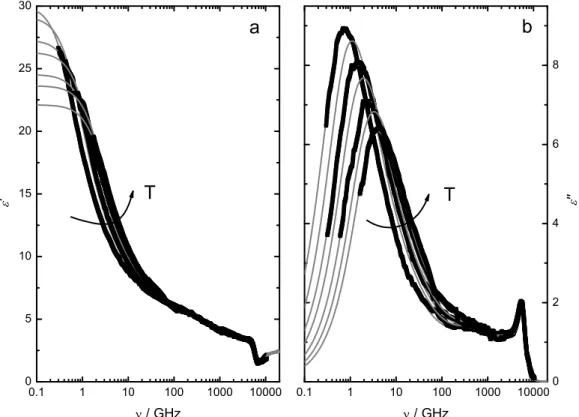
![Figure 2.2: Dielectric permittivity (a) and loss (b) spectrum of [S 222 ][TFSA] at 25 ◦ C (κ = 0.73 S m − 1 )](https://thumb-eu.123doks.com/thumbv2/1library_info/5647795.1693739/41.892.150.755.152.590/figure-dielectric-permittivity-loss-spectrum-s-tfsa-c.webp)


![Figure 3.17: Effective dipole moments, µ eff,1 ( ) and µ eff,1 ( N ) obtained via Eq. 1.52 from S 1 and S 2 , of [C 1 Im][HOAc] as a function of T](https://thumb-eu.123doks.com/thumbv2/1library_info/5647795.1693739/94.892.203.715.160.560/figure-effective-dipole-moments-eff-obtained-hoac-function.webp)
