ICES Cooperative Research Report

(1)

Best practices for the

provision of prior information

for Bayesian stock assessment

(2)

N O . 328

O ^CTOBER 2015

Best practices for the provision of prior information for Bayesian stock assessment

Editor

Atso Romakkaniemi

Authors

Charis Apostolidis • Guillaume Bal • Rainer Froese • Juho Kopra Sakari Kuikka • Adrian Leach • Polina Levontin • Samu Mäntyniemi Niall Ó Maoiléidigh • John Mumford • Henni Pulkkinen

Etienne Rivot • Atso Romakkaniemi• Vaishav Soni

Konstantinos Stergiou • Jonathan White • Rebecca Whitlock

(3)

International Council for the Exploration of the Sea Conseil International pour l’Exploration de la Mer

H. C. Andersens Boulevard 44–46 DK-1553 Copenhagen V

Denmark

Telephone (+45) 33 38 67 00 Telefax (+45) 33 93 42 15 www.ices.dk

info@ices.dk

Recommended format for purposes of citation:

Romakkaniemi, A. (Ed). 2015. Best practices for the provision of prior information for Bayesian stock assessment. ICES Cooperative Research Report No. 328. 93 pp.

Series Editor: Emory D. Anderson

The material in this report may be reused for non-commercial purposes using the recommended citation. ICES may only grant usage rights of information, data, images, graphs, etc. of which it has ownership. For other third-party material cited in this report, you must contact the original copyright holder for permission. For citation of datasets or use of data to be included in other databases, please refer to the latest ICES data policy on the ICES website. All extracts must be acknowledged. For other reproduction requests please contact the General Secretary.

This document is the product of an Expert Group under the auspices of the Interna- tional Council for the Exploration of the Sea and does not necessarily represent the view of the Council.

ISBN 978-87-7482-174-8 ISSN 1017-6195

(4)

Contents

Executive summary ... 1

1 Introduction: why priors are logically necessary ... 3

1.1 Scientific reasoning in stock assessment for fishery management ... 3

1.2 The basic concepts of Bayesian inference and the role of prior information ... 5

1.3 Worked example of a Bayesian stock assessment ... 7

1.4 The aim of the report ... 15

2 The nature of different information sources ... 17

2.1 Data …….. ... 17

2.1.1Choice of prior probability distribution ... 17

2.1.2Influence of past studies and scientific understanding ... 18

2.1.3Sample size ... 18

2.1.4Priors for unobserved values and parameters. ... 20

2.2 Literature ... 21

2.2.1Introduction ... 21

2.2.2What information to collect ... 22

2.2.3Publication bias ... 23

2.3 Online databases ... 24

2.3.1The nature of databases in the context of this work... 24

2.3.2What makes a database a suitable source of information ... 25

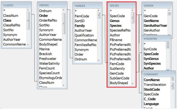
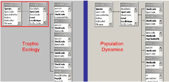
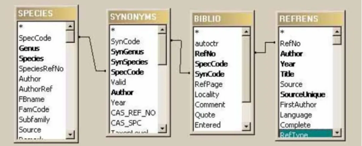
2.3.3Biological information from FishBase ... 25

2.3.4Biological information from SeaLifeBase ... 29

2.3.5Description of the ICES DATRAS database ... 30

2.3.6. Description of the ICES stock assessment database ... 32

2.4 Experts ... 33

2.4.2Selection of experts ... 34

2.4.3Potential sources of bias ... 35

2.4.4Training of experts ... 37

3 Methods ... 39

3.1 Introduction to methods ... 39

3.2 Hierarchical modelling ... 41

3.2.1Exchangeable hierarchical models... 43

3.2.2Choice of prior on hyperparameters ... 46

3.2.3Using covariates in partially exchangeable models ... 46

(5)

3.2.4Modelling correlation between biological parameters ... 49

3.3 Getting priors from FishBase ... 51

3.4 Eliciting expert opinion ... 54

3.4.2The elicitation process ... 54

3.4.3Expert elicitation tools with examples ... 60

3.4.4Combining the opinions of multiple experts (mathematical aggregation) ... 64

3.5 Bayesian belief networks ... 68

4 Summary: impacts and interpretation ... 71

5 Future research needs ... 73

6 Acknowledgements ... 75

7 References ... 76

Annex 1: BUGS/JAGS code for estimation of slope at origin of Beverton– Holt stock–recruit function (Example 3.2.1) ... 84

Annex 2: Derivation of priors for Beverton–Holt and Ricker stock– recruitment models using inputs to the ECOKNOWS stock– recruitment elicitation tool (Section 3.4.3.1) ... 85

Annex 3: Methods to obtain priors for parameters of normal and double normal selectivity curves (Section 3.4.3.2) ... 87

Annex 4: Equations used to derive priors using experts’ input in the R selectivity elicitor tool (Section 3.4.3.2) ... 89

Annex 5: BMA example using JAGS (Section 3.4.4) ... 91

Author contact information ... 92

(6)

Executive summary

This manual represents a review of the potential sources and methods to be applied when providing prior information to Bayesian stock assessments and marine risk analysis. The manual is compiled as a product of the EC Framework 7 ECOKNOWS project (www.ecoknows.eu).

The manual begins by introducing the basic concepts of Bayesian inference and the role of prior information in the inference. Bayesian analysis is a mathematical formalization of a sequential learning process in a probabilistic rationale. Prior information (also called ”prior knowledge”, ”prior belief”, or simply a ”prior”) refers to any existing relevant knowledge available before the analysis of the newest observations (data) and the information included in them. Prior information is input to a Bayesian statistical analysis in the form of a probability distribution (a prior distribution) that summarizes beliefs about the parameter concerned in terms of relative support for different values.

Apart from specifying probable parameter values, prior information also defines how the data are related to the phenomenon being studied, i.e. the model structure. Prior information should reflect the different degrees of knowledge about different parameters and the interrelationships among them.

Different sources of prior information are described as well as the particularities important for their successful utilization. The sources of prior information are classified into four main categories: (i) primary data, (ii) literature, (iii) online databases, and (iv) experts. This categorization is somewhat synthetic, but is useful for structuring the process of deriving a prior and for acknowledging different aspects of it.

A hierarchy is proposed in which sources of prior information are ranked according to their proximity to the primary observations, so that use of raw data is preferred where possible. This hierarchy is reflected in the types of methods that might be suitable – for example, hierarchical analysis and meta-analysis approaches are powerful, but typically require larger numbers of observations than other methods. In establishing an informative prior distribution for a variable or parameter from ancillary raw data, several steps should be followed. These include the choice of the frequency distribution of observations which also determines the shape of prior distribution, the choice of the way in which a dataset is used to construct a prior, and the consideration related to whether one or several datasets are used. Explicitly modelling correlations between parameters in a hierarchical model can allow more effective use of the available information or more knowledge with the same data. Checking the literature is advised as the next approach. Stock assessment would gain much from the inclusion of prior information derived from the literature and from literature compilers such as FishBase (www.fishbase.org), especially in data-limited situations. The reader is guided through the process of obtaining priors for length–weight, growth, and mortality parameters from FishBase. Expert opinion lends itself to data-limited situations and can be used even in cases where observations are not available. Several expert elicitation tools are introduced for guiding experts through the process of expressing their beliefs and for extracting numerical priors about variables of interest, such as stock–recruitment dynamics, natural mortality, maturation, and the selectivity of fishing gears. Elicitation of parameter values is not the only task where experts play an important role; they also can describe the process to be modelled as a whole.

Information sources and methods are not mutually exclusive, so some combination may be used in deriving a prior distribution. Whichever source(s) and method(s) are chosen, it is important to remember that the same data should not be used twice. If the

(7)

plan is to use the data in the analysis for which the prior distribution is needed, then the same data cannot be used in formulating the prior.

The techniques studied and proposed in this manual can be further elaborated and fine-tuned. New developments in technology can potentially be explored to find novel ways of forming prior distributions from different sources of information. Future research efforts should also be targeted at the philosophy and practices of model building based on existing prior information. Stock assessments that explicitly account for model uncertainty are still rare, and improving the methodology in this direction is an important avenue for future research. More research is also needed to make Bayesian analysis of non-parametric models more accessible in practice. Since Bayesian stock assessment models (like all other assessment models) are made from existing knowledge held by human beings, prior distributions for parameters and model structures may play a key role in the processes of collectively building and reviewing those models with stakeholders. Research on the theory and practice of these processes will be needed in the future.

(8)

1 Introduction: why priors are logically necessary Samu Mäntyniemi and Atso Romakkaniemi

1.1 Scientific reasoning in stock assessment for fishery management

ICES advises competent authorities on marine policy and management issues related to the sustainable use of living marine resources and the impacts of human activities on marine ecosystems. In order to achieve this for fishery management, experts for a fish stock carry out a scientific analysis to estimate, where possible, historic and current fishing mortality, recruitment, and population size. For most stocks with population size estimates, experts can forecast future stock size as a function of a management action (e.g. catch) and calculate what action would lead to a desired management objective (e.g. fishing mortality not exceeding that corresponding to maximum sustainable yield). The estimate of current population size is the starting point for forecasting;

thus, it has a central role in the process (ICES, 2013).

Given suitable technology, current population size could, in principle, be observed and known without error. In practice, it cannot be directly observed and needs to be in- ferred from indirect and incomplete information. This inference (estimation) is based on what scientists making the assessment believe about the relationship between true population size and observable information.

In contrast to current population size, future consequences of management actions cannot be observed, but can only be imagined (predicted). The result of this prediction depends, again, on the understanding of the scientists making the assessment.

The key point to acknowledge is that estimation and prediction require human interpretation of available information. This interpretation obviously differs between scientists and their amount of experience and knowledge. Differences in interpretation are often linked to (even minor) differences in the exact areas of specialization and experience, which lead scientists to approach research questions from slightly different per- spectives. Because of the importance of this expertise, stock assessment tasks are typically entrusted to groups of experts who comprise the membership of ICES stock assessment working groups.

Broadly standardized approaches across stocks may either fail or be suboptimal because they cannot sufficiently recognize the specificity of each fish stock, and information available on individual stocks also varies (ICES, 2013).

In other words, stock assessment is always, regardless of the analytical methods used, a subjective interpretation of observed data made by a group of experts. In this context,

“subjective” refers to things that exist only in the human mind, and “objective” refers to the actual state of the physical world. This means that only the raw observations can be regarded as objective facts. Any inferences about unobservable phenomena, such as stock size, require a human assumption about the relationship between stock size and observed data.

In this context, subjectivity does not entail or imply that experts would be invited to consider their personal preferences and valuation of a stock’s status or their political views about how a stock should be managed. It is only their personal (i.e. subjective) scientific experience and understanding that are sought in synthesizing their existing knowledge and interpretation of observed data. Experts are expected to place themselves into a neutral and independent position regarding stock assessments and to use their personal knowledge (i.e. expertise) honestly. In everyday language, experts are

(9)

expected to be objective when assessing the status of a stock using their own subjective scientific knowledge.

In principle, a stock assessment working group could “eyeball” the data spreadsheets, discuss with their colleagues, and use their collective wisdom to derive an honest and independent assessment of the stock without using any analytical methods. However, most assessment problems are too complex for the human mind to grasp as a whole.

Some form of predefined logic, organized analysis, and synthesis is usually necessary to perform the task itself and also for the transparency of the expert group’s work.

Use of mathematical models has a long history in fishery stock assessment. They have been used to organize and structure the thinking of expert groups. The types of models used have ranged from yield-per-recruit analysis to virtual population analysis and further towards integrated state–space models. Modelling practices have been influ- enced by developments in theoretical population dynamics and statistical data analysis. The purpose of statistical data analysis is to describe a set of observed data with the fewest parameters without losing too much of the structure of the original data. Trans- ferring this approach to stock assessment has led to the idea that the parameters of biological population dynamics models should all be statistically estimable from stock assessment data. However, biologically realistic population dynamics models tend to have so many parameters that their estimation from most stock assessment datasets is impossible. A common attempt to resolve this problem has been to reduce the number of estimated parameters by simplifying the model structure and then assume that some of the parameters are not uncertain, but are instead known exactly. The parameters still treated as unknown after this process can be estimated from the data, but at the cost of having decreased the biological credibility of the population dynamics model and the unwarranted exclusion of part of the uncertainty. Knowledge used to finalize model parameters usually comes from the expertise of the stock assessment working group:

group members use their biological knowledge to produce best guesses for parameters, such as the natural mortality rate (M) and the maximum size of fish, by interpreting data and conclusions presented in scientific papers, reports, and biological databases.

In this way, information from outside the stock assessment database is treated as if it were exactly known, with the consequence that the information contained in the assessment data about these parameters cannot contribute to their estimation. Con- versely, similar external information for the parameters estimated within the stock assessment is often not used at all even when it is available. Interestingly, it has been common practice to treat M as fully known and fishing mortality (F) as completely unknown, even though the latter is under human control and the former is not.

The Bayesian approach to scientific reasoning has been suggested as a remedy for this dichotomy in the use of existing knowledge. Instead of having to choose whether, based on existing information, a parameter is treated as precisely known or completely unknown, the expert group has the option to describe and quantify their uncertainty about each parameter. Some of the model parameters may be reasonably well, but not exactly, known, while other parameters are less precisely understood, but not completely unknown either. Probability distributions are used to reflect the different degrees of knowledge about different parameters and the interrelationships among them.

At the heart of the Bayesian approach is the idea of presenting everything that is not known exactly as a probability distribution.

Bayesian inference has been successfully applied in a growing number of stock assessments. For example, since mid-2000, Atlantic salmon (Salmo salar) stocks in the Baltic Sea have been assessed by an ICES working group, and the consequent advice has been

(10)

provided by using sequential Bayesian analyses (Michielsens et al., 2008; ICES, 2014).

Several stocks of Pacific salmon have been assessed by Bayesian assessment models (C.

Michielsens, Pacific Salmon Commission, pers. comm.). A Bayesian version of a sur- plus production model has been applied for the assessments of northern shrimp (Pan- dalus borealis) in the Barents Sea and Greenland halibut (Reinhardtius hippoglossoides) in Iceland and East Greenland (ICES, 2012a,b).

The Bayesian approach allows rigorous specification and utilization of relevant knowledge existing outside the primary input data used in stock assessment. This knowledge goes by various names: ”prior information”, ”prior knowledge”, ”prior belief”, or simply ”prior”. The next section presents the basic concepts and terminology of Bayesian statistical inference. Readers not familiar with the Bayesian approach should acquaint themselves with this information in order to be able to fully absorb the contents of this report.

1.2 The basic concepts of Bayesian inference and the role of prior information

In Bayesian analysis, the concept of probability is used to measure how strongly a person believes a particular hypothesis to be true. These hypotheses can consider past and future size of the fish stock, parameters of the population dynamics model, and different causal relationships represented by different model structures. A fundamental assumption is that one true stock size exists, and the Bayesian probability is used to express what a person thinks about this value. In other words, stock status exists objectively, but knowledge about it is inherently subjective without an objectively true value. For causal models and their parameters, such as F and M, the distinction between subjectivity and objectivity is not equally clear. Causal models and their parameters are also constructions of the human mind, but can be seen to represent an accepted version of reality; accordingly, they can be thought to have one true value which the person may not know exactly.

Bayesian probability is personal and, therefore, requires specification about whose probability is being used. In the case of ICES stock assessment, the most natural unit is the group of experts. The outcome of Bayesian stock assessment made by an expert group is a set of probability distributions describing their beliefs about the future status of the fish stock under each alternative management action. Ideally, these distributions summarize everything that the group knows, including the group’s interpretation of the stock assessment data. The group has typically used a variety of modelling techniques to organize their thinking and to keep the inferences logical and transparent.

Probabilities given by the expert group cannot be challenged; they represent what this particular group thinks, and different probabilities would be expected from another group. This is the key feature of the assessment; it is the honest view of this particular group of trusted experts. If the expertise was not expected to affect the assessment, Chinese berry pickers could be hired to compile the assessment of European fish stocks.

Bayesian inference can perhaps be most easily understood as a learning or inductive process. Let us consider a phenomenon which, at first, we “know” nothing about (we have no prior beliefs whatsoever about the matter, which leads us to consider that all possible hypotheses are equally probable). When making our very first observation of the phenomenon, we intuitively realize that:

 Before making the first observation, any state of the nature of the phenomenon is considered to be equally probable;

(11)

 Given the observation, we then want to consider whether a particular state or states of the nature of the phenomenon can be considered to be more probable than others;

 Based on only one observation, we are still very uncertain about the phenomenon.

By the above process, we update our knowledge about the phenomenon. This learning process can be formalized using the Bayes’ theorem (Berger, 1985; Gelman et al., 2004):

𝑃(𝐻 = ℎ𝑖|𝐸 = 𝑒) =∑ 𝑃(𝐸=𝑒|𝐻=ℎ^{𝑃(𝐸=𝑒|𝐻=ℎ}_𝑗 ^𝑖^{)×𝑃(𝐻=ℎ}_𝑗)×𝑃(𝐻=ℎ^𝑖⁾_𝑗) (1) The denominator in equation (1) is a sum over all the possible hypotheses and, therefore, only depends on the data. The Bayes theorem is, therefore, often written in its simpler and unnormalized form:

𝑃(𝐻 = ℎ𝑖|𝐸 = 𝑒) ∝ 𝑃(𝐸 = 𝑒|𝐻 = ℎ_𝑖) × 𝑃(𝐻 = ℎ𝑖) (2) Here, ℎ𝑖 stands for a particular hypothesis in a set of hypotheses (ℎ1, … , ℎ𝐽) to be examined and 𝑒 stands for evidence (observation or data). 𝑃(𝐻 = ℎ𝑖|𝐸 = 𝑒) is the probability that the hypothesis ℎ𝑖 is true given the evidence, i.e. the posterior probability. 𝑃(𝐸 = 𝑒|𝐻 = ℎ𝑖) is the probability of observing the data 𝑒 given the hypothesis ℎ𝑖 is true (i.e.

the likelihood). 𝑃(𝐻 = ℎ_𝑖) is the prior distribution, representing prior knowledge about the hypothesis. In the situation described above, our prior knowledge is ”uninforma- tive”, i.e. we set the same probability for this hypothesis to be true as for any other plausible ones. When we acquired the first observation, we could not avoid going through the inductive process described above, be it consciously or subconsciously.

The principle of Bayesian conditionalization (Howson and Urbach, 1993) states that as soon as we have new evidence, we update our belief (knowledge) about the hypothesis.

Consider now that after updating our knowledge with the first observation, we obtain a new observation. Again, we intuitively go through the previous steps of induction.

This time, we realize that we want to update our knowledge based on the new observation without forgetting the information included in the first observation. Hence, our prior distribution must logically be informative. That is, the prior 𝑃(𝐻 = ℎ𝑖) corresponds to the knowledge that we had after the first observation. After updating with the new observation, the resulting posterior distribution contains the information included in both observations. Although this example of Bayesian inference is, of course, naive, it helps us to appreciate that very seldom is there no prior knowledge about the matter that we want to examine. Therefore, it is often clearly reasonable to use an informative prior distribution in the process instead of trying to ignore or pretend that it does not exist.

A practical problem arises, however, in specifying and quantifying prior information (i.e. how to do this?). Researchers usually base most of their knowledge on information from published literature, earlier studies, pilot experiments, etc. One way to quantify prior information is to conduct an analysis of the existing, documented observations.

This may be performed by using primary data, if available, or by conducting a meta- analysis of research results published in the literature. Online databases may help in the compilation of relevant information from the literature, and they may also include processed information not published elsewhere (e.g. detailed results of analyses car- ried out in ICES assessment working groups). If information relevant for quantifying prior knowledge is diverse and/or non-commensurate as such, elicitation of expert opinions may be utilized.

(12)

1.3 Worked example of a Bayesian stock assessment

In this section, we introduce the concepts and logic of Bayesian inference in the context of a simple stock assessment example. We walk through the steps of solving the problem using Bayesian inference and also compare the approach to classical (or fre- quentist) statistical approaches based on maximum likelihood that might have been used with this problem.

Our problem is to infer the size of a fish population (𝑁) using the method of removal sampling: fish are removed from the population in successive passes, with knowledge about the fishing effort used at each pass (Mäntyniemi et al., 2005; Rivot et al., 2008).

The Bayesian approach starts by problem framing: what are the relevant variables?

Obviously the population size (N) must be involved and also the number of fish caught (ci) at each pass i. Clearly, fishing effort ( ) and efficiency of the fishing technique (q) need to be taken into account. To keep the example simple, we assume that there are no births or deaths occurring during the sampling experiment.

The next step is to establish the causal connections between the relevant variables. It is a useful practice to draw a picture where all the variables are connected using arrows that point from causes to effects. The resulting pictures are called directed acyclic graphs (DAGs) (Spiegelhalter et al., 1996). The DAG of this problem (Figure 1.1) shows that the first catch ( ) is caused by the initial abundance, fishing effort, and the efficiency factor. The catch obtained on the second pass depends on the same variables, but also the catch removed from the population on the first pass is affecting it.

Figure 1.1. Directed acyclic graph of the removal fishing problem. Round shapes denote uncertain quantities, boxes represent known or controllable quantities, and arrows denote the direction of the causal relationship.

So far, we have used our existing understanding of the problem and created a mind map about how we think the problem works. The next phase is to start defining the mind map in more detail. How well do we already know what the values of these variables are? The Bayesian approach is to use probability statements for this purpose;

nearly impossible values should be given smaller probabilities than values that we regard more credibly. Another way of thinking about the existing knowledge of a particular value, e.g. population size, is to consider the degree of disbelief; how surprised would we be if the true population size were actually 1000?

Information by which we would judge the degree of belief (or disbelief) can stem from multiple sources. Our minds could interpret data observed somewhere else in a similar situation and process the information we have adopted from the scientific literature or from discussions with colleagues. Our theoretical understanding of the subject area is likely working as “glue” by which we would synthesize past experience into a set of

N q

C₁

C₂

C₃ E

(13)

probability statements about population size and other parameters of interest. The purpose of this document is to discuss the processes and practices for deriving and formulating existing knowledge as a probability distribution. These distributions are called prior distributions or simply “priors”.

In practice, priors typically have a parametric form, which means that the shape and location of the distribution is determined by one or more parameters. Based on those parameters, probabilities for all potential values of the variables can be calculated.

Thus, it is commonplace to use well known distributions such as the normal and log- normal distributions to describe existing knowledge.

In this example, we use a log-normal distribution for population size (Figure 1.2, upper-left caption). The most credible population size is 170 individuals. Population size is believed to lie between 106 and 376, with probability 0.8.

Fishing efficiency is also thought to affect catches. But, unlike population size, the meaning of “fishing efficiency” is not that clear and requires a more rigorous definition.

For this example, we can think of the chance of capturing a fish as something that increases when fishing effort (E) increases. Following the long tradition in stock assessment modelling, we define

(3) and consequently regard as the instantaneous fishing mortality rate and q as catch- ability.

Now, we go back to defining the bits and pieces of our graphical model. We assume that, before collecting the data, effort is under our control and is not an uncertain quan- tity. Compared to N and q, catches are different; there are arrows pointing to these variables. This means that their values are believed to depend on the values of the other variables. Conditional probability distributions are used to describe what we think about this dependency. Catching fish is a random process. Even if we knew exactly the number of fish and the efficiency of our fishing method, we would still be uncertain about how many fish we will catch. This type of uncertainty is often called “aleatory”

because it arises from the random-looking variation in the process of which we are thinking. This is opposed to “epistemic” uncertainty that we have about N and q, which do not vary, but whose fixed value we do not know. In both cases, the uncertainty is personal and can be quantified using degree of belief-probability. If we believe that the fish react independently to fishing (i.e. there is no schooling behaviour or environmen- tal batchiness), a natural conditional prior distribution (or “sampling model”) for the catches would be the binomial distribution, which describes the number of successes in N independent trials, where each trial has the chance of success φ.

Finally, our full model specification can be written using mathematical notation

(4) where bar “|” indicates that the variable has a conditional prior distribution that depends on the uncertain parameters listed after the bar. The model includes five random variables, which means that the full Bayesian model is a five-dimensional probability distribution that encodes our current knowledge about the problem.

(14)

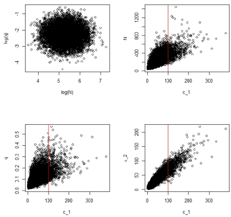
At this stage, it is worth noting that we have not observed the catches. Ideally, the model would be formulated before collecting the data, so that the model can be utilized in planning the removal process. The joint distribution can be visualized and examined by using computer simulation and taking a large sample of values from the distribution and examining the pairwise correlation plots. For example, Figure 1.2 shows that our current knowledge about the combinations of N and q is that they look independent.

This means that if we now had more knowledge about N, it would not change what we think about q. However, N and are correlated, and q and are also correlated.

This gives a hint that observing will help us to learn about both q and N. We can also see that and are correlated. Thus, if we lost the data on , we could use to infer the size of the first catch.

Figure 1.2. Prior correlations between some of the parameters in the removal sampling problem.

Red line illustrates the location of values that would be compatible with hypothetical observation .

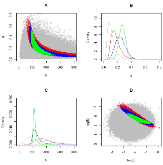
Suppose then that we start collecting the data removal by removal and examine how our thinking starts to change about population size and catchability. The first catch happens to be ; what do we now know about population size? Now, the original uncertainty about the first catch has completely disappeared. In terms of the large sample of numbers that we drew from the joint prior distribution of all parameters, this means that we should only look at those combinations where and should remove all other values. The result is shown in Figure 1.3. The red values predicted the first catch correctly and remain within the limits of possibility. We can see that, compared to the prior knowledge, a much smaller set of combinations is now realistic. It is also noteworthy that unlike before, now N and q are correlated in our minds. High N

(15)

and small q, and high q and small N, are supported by our interpretation of the observation. The joint distribution of the combination of values that are consistent with the data is called the joint posterior distribution. Looking at the variables one by one gives the marginal posterior distribution, which describes all we know about that variable.

Thus, the marginal distribution of N is of most interest in this problem. We can see that the most probable population size has moved from ca. 170 to ca. 320, while the whole posterior distribution has moved to support higher population sizes. However, the probability for a very high population size has also clearly decreased. The 80% probability interval is now 237–531; i.e. we believe that the true population is between these two values with probability 0.8.

The process of learning from observations can be intuitively described by using the simulation analogy and the idea of removing the values that are not consistent with the observations. Figure 1.3 shows how the set of parameter values gets smaller and smaller as new data are obtained, and the probability distribution describing our knowledge about N and q gets narrower. However, in addition to a simulation experiment, the way in which the probability distribution changes with new knowledge can also be presented using the well-known result of probability theory:

(5) where denotes the joint posterior distribution of N and q (red dots in Figure 1.3), is the joint prior of N and q (grey dots in Figure 1.3) and is the probability of observing for each combination of N and q. In other words, the Bayes’ rule above states that the posterior distribution of unob- served variables, given the observed values, is proportional to the product of the prior distribution and the conditional probability of observing the data at hand. In this example, the conditional probability of observations was defined using our belief that fish behave independently; consequently, the binomial distribution was used. Now that the observation is fixed at , the weight given to each combination of N and q is the probability by which this data would be observed if the combination were true.

The higher the probability of data, the more realistic the (N,q) combination seems.

Using the conditional distribution of data in this way gives rise to the so-called likelihood function, which can be seen as our personal interpretation of the objective data that were observed. By first expressing our knowledge about the observation process as a conditional distribution of potential data, we create a predefined logic by which we later interpret any specific data that we happen to obtain.

The likelihood function for a set of parameters consists of probabilities, but it does not form a probability distribution for these parameters. To make this difference clear, the values or weights given to each parameter combination are termed a “likelihood”. The widely used maximum likelihood estimation (MLE) seeks to find the combination with the highest likelihood, i.e. the values that make the observed data look most probable.

However, this is not usually the same combination that is most probable, given the observed data. For example, after observing that , the ML estimate is that the population size was N = 100 and that the catchability q is infinite so that the capture probability φ = 1. Thus, it is our prior belief that catchability should be around 0.1 that keeps the posterior distribution in a sensible range.

(16)

Figure 1.3. Joint (A and D) and marginal distributions (B and C) of the population size N and catch- ability coefficient q after observing different amount of data. Grey distribution shows the prior when no observations have been made. Red corresponds to c1 = 100, blue shows the knowledge after knowing that c¹ = 100 and c² = 50, and green is based on c¹ = 100, c² = 50, and c³ = 30.

Frequency approach

The marginal posterior of N now shows how uncertain we are about the population size after the first catch. The approach to quantifying uncertainty in classical statistics is different. Because N represents the state of nature which is assumed constant when collecting the data, it does not have a frequency probability distribution. However, it is possible to think about other estimates that could potentially realize. But this sce- nario requires hypothetical values to be assumed for N and q; otherwise, the frequency distribution for other potential data does not exist. It is common practice to use the ML estimates obtained from real data and use them as true values; it is then possible to calculate the distribution of potential data and also examine how the potential estimates would vary. Our example case is interesting: now that and , the ex- pected value of potential catches is 𝛮̂[1 − 𝑒𝑥𝑝(−𝑞̂)] = 100 and the variance is 𝛮̂[1 − 𝑒𝑥𝑝(−𝑞̂)]𝑒𝑥𝑝(−𝑞̂)⁡= 0, so we think that the data that we observed are actually the only data we could have observed and, consequently, that our potential maximum likelihood estimates would also not vary. This problematic situation arises from the idea of maximum likelihood estimation and from the practice to use that estimate as if it were the true state of nature. This situation reveals a major difference between Bayes- ian and classical statistical inference. Bayesian inference is measuring uncertainty

(17)

about the parameters themselves, whereas the frequency approach is bound to assess how potential new estimates would vary when some known values for the parameters have first been assumed.

When the second fishing pass was also made, was observed, and the question is what we now think about population size? The answer is again a posterior distribution for N, which we can obtain in the simulation example by accepting only those combinations of red dots, for which . These values and the resulting marginal distributions are shown in blue. Alternatively, we could start from the sample from prior (grey) and choose values that predicted and . In analytical terms, the Bayes’ rule can be used sequentially by taking the posterior based on the first catch as the prior for the second catch

(6) or by starting from the original prior and analyzing the whole data set at once

(7) The posterior distribution of the population size is now more peaked and covers a narrower range of values, indicating that we now have a clearer idea about population size. The most probable value is ca. 230 and almost all of the probability mass is concentrated between 180 and 400.

The probability of obtaining these two catches would be highest if N = 195 and q = 0.36, so this pair of values is the maximum likelihood estimate. Again, probability statements about population size and catchability are only possible within the Bayesian approach.

At this point, however, other potential maximum likelihood estimates would vary if we assumed that the observed estimate was the true state of nature. This variation can be examined by using parametric bootstrapping; by assuming that the true values are N

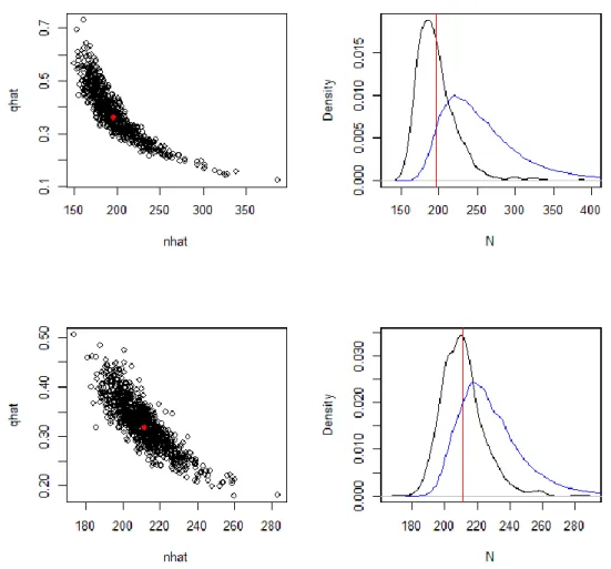
= 195 and q = 0.36, we can generate a large number of potential datasets and calculate the ML estimate from each dataset. Figure 1.4 shows the results of such an analysis. If population size were really 195, the potential ML estimates would vary around that value so that the true value would be the mean of all estimates. The joint distribution of ML estimates for N and q has a banana shape that resembles the joint posterior distribution of N and q in Bayesian analysis. It is worth noting that if N = 195, the most frequently occurring ML estimate would be ca. 180 (not 195), and that ca. 60%

of the ML estimates would be smaller than the assumed true population size.

(18)

Figure 1.4. Frequency distributions of potential maximum likelihood estimates (black dots and lines) based on the observed maximum likelihood estimates (red dots and lines). Upper row in- cludes first two catches and the lower row shows the case with all three observations. Posterior distributions of the population size (blue) are overlaid for comparison.

After making the last observation c³ = 30, the marginal posterior distribution of N is concentrated to an even narrower range (190–280) than before (Figure 1.3), but the most probable population size has not changed from 220. The marginal distribution is the final result of our analysis after observing the three sequential catches.

After these three observations, the maximum likelihood estimate of the population size is N = 211, q = 0.32. If these were the true values, then other potential maximum like- lihood estimates would vary less in comparison to the case where only two sequential catches were hypothesized. The potential estimates would still be correlated, but less than with only two catches. With three catches and assumed true values of N = 211, q

= 0.32, the most frequently occurring ML estimate for N would be 210. The frequency distributions of potential point estimates are quite often misinterpreted as if they were posterior distributions of the actual parameters based on the observed data. Figure 1.4 shows the marginal posterior distribution of N from the Bayesian analysis overlaid with the distribution of potential ML estimates obtained assuming that the observed ML estimates were the true values. It can be immediately seen that the distributions do not have the same shape and location, but it is even more important to realize that

(19)

the interpretation of the x- and y-axes are very different. For the posterior distribution of N, the x-axis shows all the alternative true population sizes, and the y-axis shows the degree of belief assigned to each of these values based on prior knowledge and three successive catches. For the frequency distribution, the x–axis does not represent the alternative true population sizes, but alternative maximum likelihood estimates that could be potentially observed if the observed maximum likelihood estimate (red line) were the true value. The y-axis shows the relative frequencies of these estimates, after repeating the fishing process for a very large number of times. In other words, the fre- quency distribution is not trying to assess the true population size, but considers a large sample of new point estimates.

The interpretations can be bridged in the following way. The blue line shows the prob- ability of each true population size and, therefore, also shows how credible the observed ML estimate is compared to other alternative true population sizes. In this case, the credibility is quite high, but not the highest of all.

The joint distribution of q and N still shows some correlation, which hints that a further reduction in uncertainty about N would still be possible if more information about catchability could be obtained. Whether the current uncertainty is too large or not does not belong to the field of Bayesian inference; the uncertainty is what it is and does not possess any value in itself.

Whether attempts should be made to further reduce uncertainty always depends on the context. The most rigorous way to analyze the need for collecting more data is to adopt the Bayesian decision-analysis approach (Raiffa and Schlaifer, 1961) where the costs of data collection can be contrasted with expected gains of managing with and without the potential new data (McDonald and Smith, 1997; Mäntyniemi et al., 2009).

Such a value-of-information (VoI) concept is tightly linked to the honest use of prior information in fishery stock assessment and management. Whenever the expert group intentionally leaves some information unutilized in the Bayesian stock assessment (uses too flat prior distributions compared to actual knowledge), the value of any new information will become overestimated. Whenever the group pretends to know parameters that are not well known (e.g. by fixing natural mortality), the value of any new information will become underestimated (Mäntyniemi et al., 2009).

Terminology

Belief. Knowledge that includes uncertainty. The word ”belief” is used to underline the inherent subjectivity of any uncertain knowledge.

Probability distribution. Also called probability density function (pdf) when it is spec- ified as a function. A parameter the value of which is not exactly known has a probability distribution. The probability distribution encapsulates the current belief/knowledge about what values the parameter may have and how probable each value is. Probability distribution may be continuous or discrete.

Subjectivity. Knowledge is necessarily a personal thing and is subjective by its very nature. Our knowledge and the lack thereof are inside our mind (belief) and, therefore, are subjective. Collective knowledge is also (collectively) subjective. Subjectivity is equally present both in the Bayesian and non-Bayesian approaches. Subjectivity does not exclude neutrality, honesty, or ”unbiasness”, but rather stresses the importance to strive for them.

(20)

Objectivity. The real world outside the human mind is objective. Human knowledge is not objective, and there is no objective thinking. Therefore, objectivity only relates to

”the truth out there”.

Prior (belief/knowledge/information). Also simply called ”prior”. Existing relevant knowledge available before the analysis of the newest observations (data) and the information included in them. Prior knowledge is not fed into a statistical analysis in a form of observations, but in a form of probability distribution, which summarizes what is believed about values of the parameter of concern. Apart from specifying probable parameter values, prior knowledge is also specifying processes, i.e. defining how data are related to the studied phenomenon (model structure and sampling model).

Posterior (belief/knowledge/information). Formal synthesis of prior knowledge and new observations (data) by using Bayes’ rule results in probability distribution, which is the posterior knowledge of the parameter of concern.

Updating. The process of applying Bayes’ rule to combine prior knowledge and data.

Bayes’ rule/Bayes’ theorem. P(h|e) ∝ P(e|h)P(h). See page 6 for more details.

Uncertainty about uncertainty

The chance parameter φ is interesting because it essentially represents a certain kind of probability. However, it is not a Bayesian degree of belief, but rather a parameter that describes the behaviour of the real-world system. While Bayesian probability measures what we know about the system, this chance parameter represents the ran- domness in the system. If we imagine trying to catch an infinite number of fish, φ would represent the proportion of successes in such a situation. On the other hand, φ does not really exist in the same way as the true population size N, but exists in our minds as a property of the system. In other words, we can never observe φ directly; we can only observe counts of fish. This implies that we will always be uncertain about the (imaginary) true value of φ, which breaks down to uncertainty about catchability (q), effort ( ), or both.

Now, the Bayesian approach is to express uncertainty about these parameters using a prior distribution. This is an important case because we are using the degree of belief – probability to express what we know about a “physical” probability. This is where the Bayesian inference encapsulates the frequency probability and allows us to measure the uncertainty about it. This is not possible in classical statistics, which uses only the concept of frequency probability. On the other hand, the Bayesian approach as- sumes that everyone knows their own degree of belief and does not possess the concept of a person’s degree of belief about his or her own degree of belief. Yet another concept of probability would be needed for assessing such uncertainty.

1.4 The aim of the report

This report is a manual representing a review of the methods to be applied when providing prior information to Bayesian stock assessments and marine risk analysis. It is compiled by the ECOKNOWS project, where a critical summary of the existing methods to formulate prior information and further development of the methods is one of the essential deliverables to be provided. The manual also facilitates a better commu- nication of scientific information expressed in the form of probabilities.

(21)

Due to the application of an ecosystem approach to fishery management, there is an increasing need to expand risk-related advice to new species. Often, little or no tradi- tional stock assessment data exist about these species; hence, effective utilization of various background data and other sources of information is essential. Our report is a comprehensive handbook guiding the use of this type of information in assessment and advice, which is relevant both in data-rich target fisheries and especially in data- poor cases related to, for example, bycatch species.

As already pointed out, much research is built on more or less conscious (subjective) reasoning leading to choices or preferences regarding scientific questions to be studied, data, analyses, and conclusions. This also holds in the guidelines we present here, which are our ”posterior beliefs” based on our experience thus far and which we are offering as ”priors” for the readers. Thus, in order to be consistent with our message, we want to stress that updates to our guidelines are expected in the future¹. We also welcome any feedback on how well stated and transparent our reasoning is, or how consistent it is with readers’ own experiences.

1 The updates may arise from our own or from the readers’ future experiences and they may either confirm or refute our current understanding.

(22)

2 The nature of different information sources

Jonathan White, Guillaume Bal, Niall Ó Maoiléidigh, Konstantinos Stergiou, Samu Mäntyniemi, Atso Romakkaniemi, Rebecca Whitlock, Rainer Froese, Vaishav Soni, Polina Levontin, Adrian Leach, and John Mumford

2.1 Data

Jonathan White, Guillaume Bal, and Niall Ó Maoiléidigh

Setting an informative prior from data should be considered if only a small amount of data describing the target variable exist, or if the data in question are not believed to be representative of the true variable. This may be the case if sampling bias is sus- pected, e.g. where data are believed to give a sample estimate of the distribution rather than the true population distribution. For example, the size of fish in a commercial catch may be subject to sampling bias either from restrictions on the fishing net mesh size, hook size, or an implemented minimum take size. If the size of fish in the entire population is the target of the variable being modeled, then an informative prior of the true range of fish size in the population would be desirable. This could be determined from scientific sampling, samples taken over a longer time-series where the time-series incorporates individuals from the full population, or from the literature.

The aim is to develop a frequency distribution reflecting the true range of the variable or parameter of interest, with the weight of the distribution function concentrated around its midpoint. To this end, if the data to be applied in a model are believed to exhibit some sampling bias away from the true population (such as measurements of fish size from catches with fishing restrictions), then they should not be used in con- structing the prior. Reliance on the same data would give rise to a higher degree of certainty in the posterior than should be accepted.

In establishing an informative prior distribution for a variable or parameter from other ancillary data, several steps should be followed. The expected frequency distribution needs to be chosen that will determine the parameters needed to define the distribution within the mathematical syntax of the chosen software. For example, a normal distribution is determined by values describing the mean and standard deviation; a binomial distribution is determined by the probability of success and the number of trials; and a negative binomial distribution is determined by the probability of success and the number of successes. The choice of the frequency distribution determines the (i) shape of the distribution, (ii) range of values around the midpoint (typically chosen as the mean, median, or mode of the distribution) and also their symmetry or asymmetry, and (iii) density of values (their probability) relative to distance from the midpoint.

2.1.1 Choice of prior probability distribution

The aim of setting an informative prior distribution from data is to describe the situation – the variable of interest – as well as possible. Two main factors will determine this choice:

 prior understanding of the frequency distribution from other examples or knowledge and;

 the size of the dataset being used to set the prior, and its apparent frequency distribution.

(23)

Prior knowledge of the variable in question and scientific knowledge of general types of data are important in a priori choosing the density function for an informative prior.

The sample size of the data, however, will have the greatest influence on the choice.

2.1.2 Influence of past studies and scientific understanding

General knowledge of probability distributions, datasets of a similar nature, and experience with sets of the same type of data from different sources are likely to influence the choice of the prior distribution function. Examples of generally expected probability distributions include:

 Weight and length measurements of individuals in an age class tend to be normally or log-normally distributed.

 Numbers of males to females in a population of known total size tend to follow a binomial distribution.

 Organisms in the environment tend to be clumped or contagious in their spatial distribution; therefore, probability distributions of their counts from spatial sampling techniques (such as sweep net or quadrate surveys) tend to be strongly right skewed, following negative binomial or log-normal distributions.

 Organism distributions are sometimes regularly distributed within contagious clusters and, at this smaller scale, may display a uniform frequency distribution.

 Certain events occur with a regular temporal distribution, such as temper- ature relative to the time of day or year, or the eruptions of a geyser. In such cases, this should be reflected by the chosen probability model.

 Some weather events have a contagious temporal distribution, such as the frequency and strength of tornadoes and winds, for which the Weibull distribution has often been used to model probabilities.

Previously collected datasets of the same variable from a different source can also give valuable insight into the expected frequency distribution form. For example, length measurements of a population of a species, different from the population of interest, may be informative. While care needs to be taken doing this, it can be a useful approach. An “information donor” population should be chosen that is believed to be close to the population of interest. In this sense, the term “close” applies not only to the spatial and temporal localities of “donor” and “recipient” population estimates, but also to the value of the variable under scrutiny.

Furthermore, the general form of a frequency distribution is more robust than the actual range of its elements (or measurements). For example, while a population of the wood mouse (Apodemus sylvaticus) from a productive habitat may have a mean weight of 26 g and a population from a less productive habitat may be significantly smaller with a mean weight of 20 g, the frequency distribution (probability function) of weights of the two populations may be expected to exhibit the same shapes and forms. This will hold true for many measurement types and their classes and justifies the application of a probability distribution type based upon experience.

2.1.3 Sample size

The way in which a dataset is used to construct a prior needs consideration. Sample size is most important, as this will influence how the frequency descriptors of the data

(24)

are implemented, either using the full dataset directly or alternatively calculating or estimating descriptors of the dataset.

Large sample sets clearly are the most reliable for setting informative priors. Frequency distributions of dataset values can be used to fit expected probability distribution func- tions; then, goodness-of-fit tests are performed to choose the most appropriate form and its values to define the prior. This can lead to strongly informative priors that can be appropriate when the variable in question is very closely associated with the data used to create the prior. If, however, the data used in setting the prior represent a different population, time, or location, care should to taken to ensure they are not overly influential, as they could limit development of the posterior by being too strong and thus limit the model and its data in influencing the posterior estimate.

For smaller datasets still large enough to exhibit a discernable probability distribution type or shape, descriptors can be calculated and the frequency distribution can be examined and compared against known, expected frequency distributions, and the mean, median, mode, standard deviation, variance, etc. calculated directly.

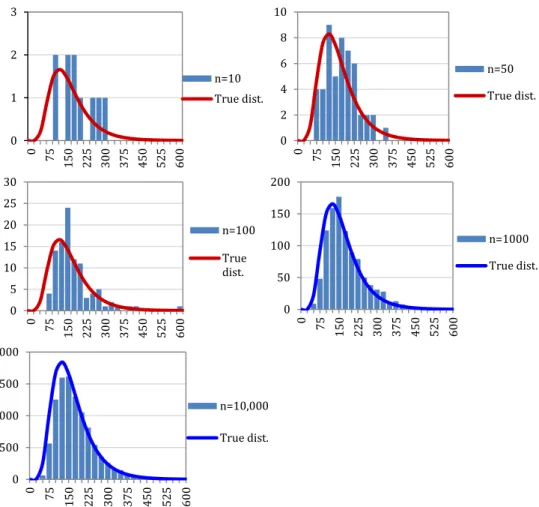
For small datasets, comprising anything below ca. 50 samples, choosing an appropriate probability distribution becomes difficult. For small datasets, the shape of the distribution function is not always apparent. Figure 2.1 shows frequency plots of values randomly drawn from a log-normal distribution (mean = 5; s.d. = 0.447) and an increasing number of drawn samples (n = 10, 50, 100, 1000, and 10 000). For the first two series of draws (n = 10 and 50) and, to an extent, the third (n = 100), the shape of the distribution is not clear, and no distinct pattern could be reliably proposed. In such cases, the basic details from the data (mean, median, standard deviation) can be calculated and applied to a prior. However, the choice of the distribution type would be left to expert opinion or prior knowledge (see above).

If small sample sizes are to be used, misspecification of the prior could result in two ways: (i) inaccuracy in the direct estimate of the distribution descriptors (mean, median, standard deviation) and (ii) from application in a model of an incorrect probability distribution type. In these cases, a balance must be reached between information arising from the data and that from expert opinion. In such instances, it is important to ensure that the informative prior incorporates the expected variability in the variable and does not force estimates to a very narrow and potentially falsely precise value.

(25)

Figure 2.1. Frequency distributions of n = 10, 50, 100, 1000, and 10 000 randomly drawn samples from a log-normal distribution with a predetermined mean of 5 and standard deviation of 0.447. The sample means and standard deviations given in Table 2.1 are included for comparison (note that for n = 10, 50, and 100, the expected distribution plots in red emphasize their difference to the ob- served sample frequencies).

Table 2.1. Sample size and associated means and standard deviations from randomly drawn sam- ples of a log-normal distribution with a predetermined mean of 5 and standard deviation of 0.447.

Frequency distributions are plotted in Figure 2.1.

Distribution n 10 50 100 1000 10 000 True values Log scale Mean 128.03 150.29 161.83 163.05 163.62 164.02 s.d. 49.285 73.334 67.344 76.687 78.026 77.194 Transformed Mean 4.765 4.904 5.001 4.993 4.994 5.000 Used to

establish distributions s.d. 0.4747 0.4674 0.4201 0.4492 0.4551 0.4472

2.1.4 Priors for unobserved values and parameters.

Unobserved model components can fall into two categories:

 Variables that are representative of a true value or count. For instance, the number of fish or their size at a specific life stage in a specific location that are not observed. These variables are true values even if not measured (i.e.

not observed).

0 1 2 3

0 75 150 225 300 375 450 525 600

n=10 True dist.

0 2 4 6 8 10

0 75 150 225 300 375 450 525 600

n=50 True dist.

0 5 10 15 20 25 30

0 75 150 225 300 375 450 525 600

n=100 True dist.

0 50 100 150 200

0 75 150 225 300 375 450 525 600

n=1000 True dist.

0 500 1000 1500 2000

0 75 150 225 300 375 450 525 600

n=10,000 True dist.

(26)

 Parameters or notional (conceptual) values that are used in mathematical modelling, but are not measurable (e.g. parameters within stock–recruitment models).

For unobserved values, informative priors can be implemented from alternative datasets if samples of the population of interest are not available. These may be scientific samples or fishing samples. Priors may also be derived from combinations of datasets if there is an expected reliable relationship among the different datasets. The criteria described above for using data in the derivation of priors apply here as well.

For parameters, the situation is similar. While the target value and its probability distribution may not be observed directly from a dataset, the combination of datasets through a relationship or model can indicate the expected probability distribution form and range [e.g. a parameter in a growth relationship, such as the growth rate (r) and carrying capacity (k) of the Beverton–Holt (1957) growth model].

If prior estimates of a value are going to be derived from two or more datasets, the conditions detailed above, namely the sample size of the dataset and the expected probability distribution form, need to be considered for each dataset. The methods presented in Section 3.2 include an appropriate toolbox for deriving priors from several datasets.

2.2 Literature

Konstantinos Stergiou, Samu Mäntyniemi, Atso Romakkaniemi, and Rebecca Whitlock

2.2.1 Introduction

Literature is an important source of information for various parameters related to the assessment of fish stocks. For instance, in a review of length-at-first-maturity of fish in the Mediterranean Sea, a region traditionally considered data-poor, information was found for 565 marine fish stocks representing 150 species (Tsikliras and Stergiou, 2014).

This is especially true of the so-called grey literature (i.e. theses, proceedings, local journals, journals that publish in languages other than English) which was not widely available before the Internet era and, until recently, was generally not included in various online bibliographic databases (e.g. Scopus, Web of Science). For instance, >60%

of the articles cited in four reviews on various biological aspects of Mediterranean marine and freshwater fish were in local, grey literature (Stergiou and Tsikliras, 2006).

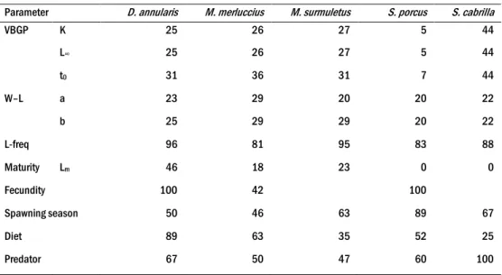
Despite the existence of large databases that accommodate the available literature and from which relevant information can be extracted (Section 2.3), the percentage of the published primary and grey literature that is not incorporated into such databases can be high (e.g. Stergiou and Moutopoulos, 2001; Stergiou and Karpouzi, 2002; Apos- tolidis and Stergiou, 2008; Tsikliras and Stergiou, 2014). For instance, within the ECOKNOWS project (www.ecoknows.eu), for the five Mediterranean case study species and the nine parameters examined, the percentage of records derived from both primary and grey literature not included in FishBase (Froese and Pauly, 2014, www.fishbase.org, version 8/2011) ranged from 0 to 100%, depending on the species and parameter (Tables 2.2 and 2.3) (Stergiou et al., 2012).