The use of rotational invariants for the interpretation of marine CSEM data with a case study from the North Alex mud volcano, West Nile Delta

(1)

Geophysical Journal International

Geophys. J. Int.(2015)201,224–245 doi: 10.1093/gji/ggv015

GJI Marine geosciences and applied geophysics

The use of rotational invariants for the interpretation of marine CSEM data with a case study from the North Alex mud volcano, West Nile Delta

Sebastian H¨olz,

¹

Andrei Swidinsky,

²

Malte Sommer,

¹

Marion Jegen

¹

and J¨org Bialas

¹

1Department for Geodynamics, GEOMAR Helmholtz Centre for Ocean Research Kiel, D-24148Kiel, Germany. E-mail:shoelz@geomar.de

2Department of Geophysics, Colorado School of Mines, Golden, CO80401, USA

Accepted 2015 January 8. Received 2015 January 7; in original form 2014 February 16

S U M M A R Y

Submarine mud volcanos at the seafloor are surface expressions of fluid flow systems within the seafloor. Since the electrical resistivity of the seafloor is mainly determined by the amount and characteristics of fluids contained within the sediment’s pore space, electromagnetic methods offer a promising approach to gain insight into a mud volcano’s internal resistivity structure. To investigate this structure, we conducted a controlled source electromagnetic experiment, which was novel in the sense that the source was deployed and operated with a remotely operated vehicle, which allowed for a flexible placement of the transmitter dipole with two polarization directions at each transmitter location. For the interpretation of the experiment, we have adapted the concept of rotational invariants from land-based electromagnetics to the marine case by considering the source normalized tensor of horizontal electric field components. We analyse the sensitivity of these rotational invariants in terms of 1-D models and measurement geometries and associated measurement errors, which resemble the experiment at the mud volcano. The analysis shows that any combination of rotational invariants has an improved parameter resolution as compared to the sensitivity of the pure radial or azimuthal component alone. For the data set, which was acquired at the ‘North Alex’ mud volcano, we interpret rotational invariants in terms of 1-D inversions on a common midpoint grid. The resulting resistivity models show a general increase of resistivities with depth. The most prominent feature in the stitched 1-D sections is a lens-shaped interface, which can similarly be found in a section from seismic reflection data. Beneath this interface bulk resistivities frequently fall in a range between 2.0 and 2.5m towards the maximum penetration depths. We interpret the lens-shaped interface as the surface of a collapse structure, which was formed at the end of a phase of activity of an older mud volcano generation and subsequently refilled with new mud volcano sediments during a later stage of activity. Increased resistivities at depth cannot be explained by compaction alone, but instead require a combination of compaction and increased cementation of the older sediments, possibly in connection to trapped, cooled down mud volcano fluids, which have a depleted chlorinity. At shallow depths (≤50 m) bulk resistivities generally decrease and for locations around the mud volcano’s centre 1-D models show bulk resistivities in a range between 0.5 and 0.7m, which we interpret in terms of gas saturation levels by means of Archie’s Law. After a detailed analysis of the material parameters contained in Archie’s Law we derive saturation levels between 0 and 25 per cent, which is in accordance with observations of active degassing and a reflector with negative polarity in the seismics section just beneath the seafloor, which is indicative of free gas.

Key words: Numerical approximations and analysis; Electrical properties; Marine electromagnetics; Gas and hydrate systems; Hydrothermal systems; Permeability and porosity.

224 ^CThe Authors 2015. Published by Oxford University Press on behalf of the Royal Astronomical Society.

at Leibniz-Institut fur Meereswissenschaften on April 29, 2015http://gji.oxfordjournals.org/Downloaded from

(2)

Rotational invariants for mCSEM data 225

I N T R O D U C T I O N

Submarine mud volcanos, which are important indicators for dy- namic processes within gas bearing sedimentary units, are a common feature in marine environments and represent surface expressions of fluid flow and gas migration systems within the seafloor (Kopf2002). Active mud volcanos show distinct geochemical sig- natures with changing salinity of pore fluids (Hensenet al.2007).

Also, large temperature gradients and occurrences of free gas (Feseker et al.2009) can frequently be observed. Since the electrical resistivity of the seafloor is mainly determined by its porosity and the electrical resistivity of the pore fluid, the latter being weakly coupled to the temperature of the pore fluid (Fofonoff1985), electromagnetic methods offer a promising approach to gain insight into a mud volcano’s internal structure. Occurrences of fresh water, gas, gas hydrates or hydrocarbons decrease the saturation of the conductive pore fluid and, thus, lower the bulk resistivity. In addition the precipitation of authigenic carbonates to the seafloor at seep sites may appear as resistive anomaly, provided they form car-

bonate blocks or crusts which are sufficiently large with respect to the scale length of electromagnetic investigations. Consequently, a marine controlled source electromagnetic (mCSEM or CSEM from now on) experiment at ‘North Alex’,a mud volcano in the West Nile Delta, was scheduled to take place in November 2008.

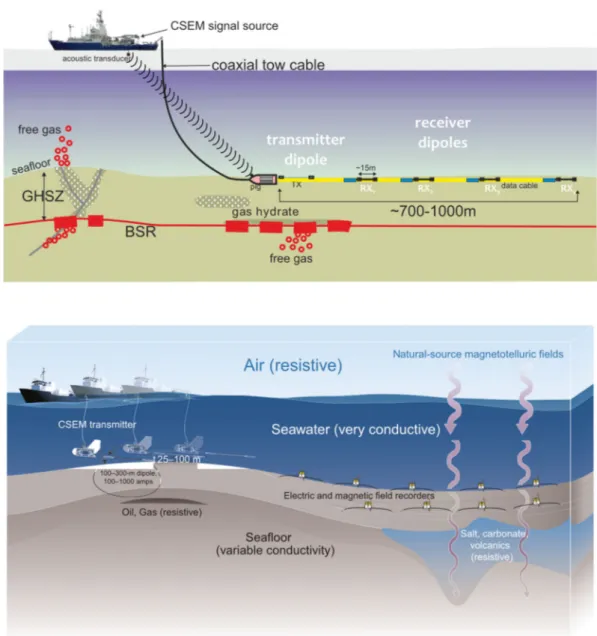
The original plan for the CSEM experiment was to use the bottom towed system developed by the University of Toronto described in Schwalenberget al.(2010) (Fig.1, bottom panel). In preparation of the experiment it became clear that this system would not be suitable for investigations, since occurrences of carbonates, existing cable installations and various deployed scientific instruments would not have allowed for a safe operation.

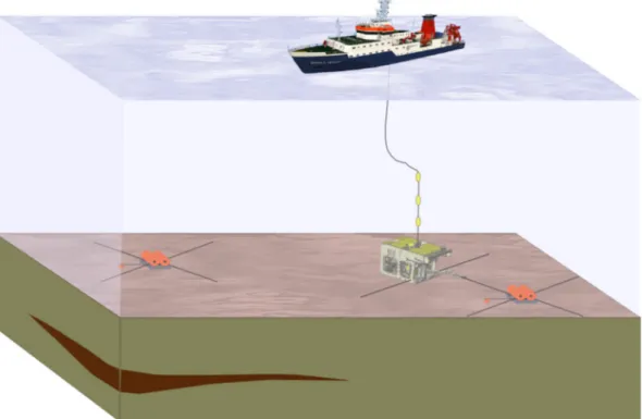
For investigations at the North Alex we therefore had to implement a novel type of experiment, for which we used a remotely operated vehicle (ROV) to deploy the transmitter (Fig.2). The ex- perimental setup was inspired by the up to then unique CSEM experiment conducted at the TAG hydrothermal mound by Cairns et al.(1996). They had used the submersibleAlvinto deploy a stationary, autonomous receiver onto the TAG hydrothermal mound.

Figure 1. Conventional CSEM experiments with a cable-based system with fixed geometry (top panel, from Schwalenberget al.2010) or a ‘flying’ source and a stationary receiver array (bottom panel, from Constable2010).

(3)

Figure 2.Schematic sketch of WND experiment with the ROV deployed transmitter and two nodal receivers (instruments are shown in Fig.10). In the experiment transmitter and receivers are arbitrarily oriented. A sketch of the general geometry of the experiment is given in Fig.3. Modified from Sommer et al.(2013).

Alvinwas then used to move a transmitter around in the survey area.

Their original plan to deploy both receiver and transmitter with two perpendicular antennas (3 m) each, had to be abandoned due to technical problems. Instead, the experiment was carried out with only one dipole on each, receiver and transmitter. The transmitter was operated with a single transmitter polarization at each site only (Cairns & Edwards, personal communication, 2014).

Apart from avoiding the hazards mentioned above, this style of experiment, where a submersible or ROV is used to move around the transmitter, offers the unique chance to excite several polarizations at every transmitter site. This is quite different to the bottom towed system (Fig.1, top panel), which is only capable of exciting a single polarization at each transmitter site as well as for other common CSEM systems like the Scripps system described in Constable (2010) (Fig.1, bottom panel), newer developments like the Vulcan System (Weitemeyer & Constable2010) or the surface towed system described by Anderson & Mattson (2010). Generally speaking, the Scripps system could also be used in experiments, where two transmitter polarizations are collected. However, this is not standard which is due to the fact that this requires a different style of CSEM experiment, in which cross tows across the receivers are used to excite the second polarization, which is costly to implement (Constable2010).

For these common systems, which excite a single transmitter polarization at each location a first pass interpretation of measured fields at receiver stations is usually carried out using the radial component of the electric field, whereas the azimuthal data is often not considered. However, recent publications recognize the fact that the collection of both polarizations would generally be advisable, for example in terms of resolving possible effects of 3-D anisotropic structures (Newmanet al.2010).

Measurements with two transmitter polarizations require different ways of processing and interpretation for a first-pass interpreta-

tion. We are currently establishing a work-flow for such data, which relies on the concept of rotational invariants. The work-flow is as follows:

1. Construction of rotational invariants from marine CSEM data measured with non-parallel transmitter polarizations.

2. Derivation of apparent resistivities from the invariant data.

3. Interpretation of rotational invariants in terms of 1-D layered models of the seafloor.

4. Dimensionality analysis of rotational invariants.

5. Interpretation of rotational invariants in terms of 3-D mod- elling and inversions.

The calculation of apparent resistivities from one of the rotational invariants, which is useful for the fast imaging of data (step 2), is published in a companion paper (Swidinskyet al.2015). The dimensionality analysis (step 4) and the 3-D interpretation (step 5) are both work in progress and will be included in future publications.

Within this paper steps 1 and 3 are covered in two main sections:

The first section deals with theoretical aspects of rotational invariants, first demonstrating how rotational invariants are constructed from measured data (step 1). After introducing the general concept, the sensitivity of rotational invariants is tested on a basic 1-D model, which resembles the measurement geometry of CSEM measurements at the mud volcano and the model resolution in the interpretation of rotational invariants is compares to the resolution, which can be achieved in the interpretation of a data set, which uses a single transmitter polarization only.

In the second section of this paper a proof of principle for the invariant approach is given by application to the CSEM data acquired during an experiment at the ‘North Alex’ mud volcano. The results of the CSEM data are tied into results from seismics and additional geoscientific data and finally interpreted in terms of gas saturation levels and structural features of the mud volcano.

(4)

R O T AT I O N A L I N VA R I A N T S Theory

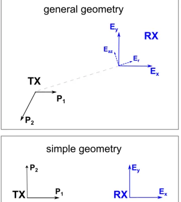
Considering a CSEM experiment with two non-aligned transmitter (TX) dipoles with dipole momentsP₁andP₂at a given TX location (Fig.2, top panel), it is immediately clear that field components at a given receiver (RX) are usually not recorded as unique radial (Er) or azimuthal (Eaz) fields, but rather four trigonometric combinations of these fields (Constable & Cox1996).

Of course it is possible to simply reconstruct the radial as well as the azimuthal component for each of the two transmitter polarizations. However, for a first-pass 1-D interpretation this poses two problems:

1. For a given transmitter location, the reconstructed radial and/or azimuthal components may not be unique and instead may differ substantially for the two polarizationsP₁ andP₂. This can be due to the 3-D resistivity distribution of the subsurface, bathymetric effects or the change in source strength for a given direction (e.g. in the radial direction) for the two transmitter polarizations.

2. The flexible placement of the TX leads to a situation where polarization directions for adjacent TX locations may vary quite substantially (compare Fig. 8), that is when comparing a given polarization from one TX location to the next the measurement error of the reconstructed radial and/or azimuthal components may vary substantially because of the changing polarization direction.

Therefore, it is advantageous to find a representation of the measured field components, which is independent of the TX and RX orientations. This is possible by the use of rotational invariants, which were introduced for land-based dc measurements by Bibby (1977,1986), applied by Risket al.(1993) and further general- ized to time-domain measurements by Caldwell & Bibby (1998).

The aforementioned authors use an approach, in which the measured electric field components, which are excited by two (or more) non-aligned TX polarizations, are normalized by the dc current density. For land-based measurements over a half-space the dc current density is independent of the distribution of resistivities in the subsurface and the authors show that the determinant of the normalized E-fields can be interpreted in terms of apparent resistivities.

A direct adaption of this concept to the marine case fails—at least in terms of producing reasonable apparent resistivities—because in the marine case the dc current flow is not independent of the resistivity of the lower half-space. However, Li & Pedersen (1994) point out that the overall concept for rotational invariants, that is the independence on the choice of the reference frame, does not depend on the general distribution of resistivities. Thus, we argue that the general framework of rotational invariants, which was derived for land-based measurements, will also hold for the marine case. In this paper, we will show that rotational invariance can be established for the marine case, since it is only necessary to normalize the measured fields by a quantity, which reflects the source geometry. In the aforementioned companion paper we show how these invariants can be used to derive an apparent resistivity, which can be used for the quick imaging of CSEM data of experiments with two transmitter polarizations (Swidinskyet al.2015).

Suppose we have an experiment, where a transmitter with two dipole polarizations and a receiver are placed horizontally onto the seafloor in an arbitrary geometry (Fig.2, right-hand side). We assume the reference frame to be aligned with thex- andy-components of the RX. For two non-aligned TX measurements with time dependent (not denoted explicitly) dipole momentsP₁ andP₂ and mea-

sured electric fieldsE₁andE₂, the accordingxy-components in this reference frame are written in matrix notation to derive a source normalized E-fieldEⁿ:

P=[P1P2]=

⎡

⎣P_x,1 P_x,2 Py,1 Py,2

⎤

⎦

E=[E1E2]=

⎡

⎣Ex,1 Ex,2

E_y,1 E_y,2

⎤

⎦→Eⁿ≡E·P⁻¹. (1)

The calculation ofP⁻¹is always possible, because the two polarizations are assumed to be non-aligned and, thus,Eⁿis well defined.

Please note that in the following the superscript ‘n’ always denotes the source normalization and not a mathematical power. For matrix elements (EijandPij), the first index (i=x,y) identifies the hori- zontal component, the second index (j=1, 2) identifies the used TX polarization.

We now consider a second coordinate system, which is rotated by an arbitrary angle with respect to the first coordinate system by using the corresponding rotation matrix. If the distance between TX and RX is larger than approximately 5×the length of the TX bipole, they may be considered as dipoles. In this case—due to the principle of superposition—the components of bothP˜andE˜ in the rotated coordinate system are described by applying the 2-D rotation matrixR:˜

P˜ =R˜⁻¹·P E˜ =R˜⁻¹·E. (2) The source normalized E-field matrix in the rotated coordinate system can be written as:

E˜ⁿ=E˜ ·P˜⁻¹=R˜⁻¹·E·P⁻¹·R˜ =R˜⁻¹·Eⁿ·R.˜ (3) It is important to note that it is the normalization by the source polarizations, which ensures thatEⁿis a second-rank tensor, similar to the rationale used in the definition of the apparent resistivity tensor by Caldwell & Bibby (1998). Even though the elements of the source normalized E-field tensor depend on the orientation of the coordinate system, rotational invariants can be defined, which are indeed independent of the orientation of the coordinate system:

I1≡det (Eⁿ)=det E˜ⁿ

=E_x,1ⁿ ·Eⁿ_y,2−E_x,2ⁿ ·Eⁿ_y,1 I2≡trace (Eⁿ)=trace

E˜ⁿ

=Eⁿ_x_,₁+Eⁿ_y_,₂ I3≡skew (Eⁿ)=skew

E˜ⁿ

=Eⁿ_x_,₂−E_yⁿ_,₁

. (4)

Additionally, we can use a combination of I1–3to define I4, which is also rotationally invariant:

I4≡I²₂+I²₃−2I1= ||Eⁿ||²= E_iⁿ_,_j2

. (5)

This invariant is simply the sum of squares of the matrix elements as defined in eq. (1). It has the advantage that it has the same dimension as I1and we will later use it in the interpretation of data.

In order to calculate invariants for simple 1-D cases, we may assume a simple geometry as in Fig.3, in which both TX and RX are aligned with the reference frame. The matrix of source normalized electric field components then simply contains the inline and broadside responses and rewriting eq. (4) yields:

I1= E_inⁿ ·E_brⁿ I₂= E_inⁿ +E_brⁿ I3=0 I4=

E_inⁿ2

+ E_brⁿ2

,

(6)

(5)

Figure 3.Map view of the general geometry (top panel) of the experiment depicted in Fig.2. Note that for the concept of rotational invariants, the two transmitter polarizations (P₁andP₂) are only required to be non-parallel.

Thus, the polarizations are depicted at a non-orthogonal angle and with different lengths for general considerations. However, in the CSEM experiment at the mud volcano the two polarizations were always nearly orthogonal and of equal dipole moment. For the calculation of rotational invariants for 1-D models we use a simple geometry (bottom panel), in which the transmitter and receiver are aligned with the reference frame. Here, polarizationP1

excites the pure inline response in receiver component Exand polarization P2excites the pure broadside response in receiver component Ey. where the superscript ‘n’ denotes the source normalization. For the 1-D case, the skew (I3) is always zero. Since we will only interpret data in terms of 1-D layered earth models in the scope of this paper, the skew invariant will not be part of the interpretation presented here, but will be evaluated within a future 3-D interpretation of the data.

It is worthwhile to note that invariants I₁and I₄do not depend on the orientation of the receiver. For invariant I1this is easy to see, since applying a rotation matrixRtoEⁿand applying the definition of I1(4) yields:

I₁=det (R Eⁿ)=det (R)·det (Eⁿ)=det (Eⁿ)=I₁. (7) Thus, any error in the orientation of the system does not propagate into these invariants.

Model curves and sensitivity study

In the following we will use (6) for calculations of invariants, thus, all calculations presented hereafter are based on the assumption of a 1-D layered lower half-space representing the seafloor and a 1-D layered upper half-space, which represents the water column with the confining air layer above. For calculations we use a For- tran code originally developed at the University of Toronto, which implements the theory described in Edwards (1997) and Scholl &

Edwards (2007). We have modified the code to allow for calcula-

tions with layered water columns and adapted the code to be directly accessible from within Matlab. For inversions, which we will show in a later section, we use the 1-D forward code in combination with the optimization methodlsqnonlinfrom the Matlab Optimiza- tion Toolbox, which relies on a trust-region-reflective algorithm that is based on the interior-reflective Newton method described in Coleman & Li (1994,1996).

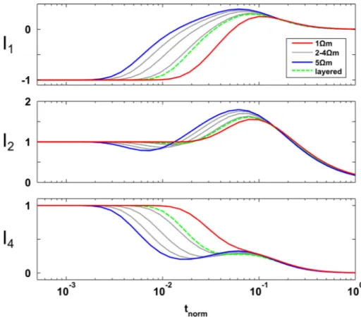
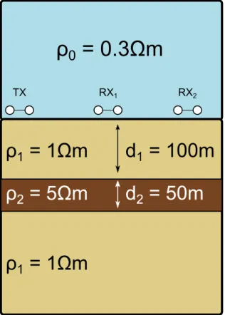
To demonstrate how these invariants behave (Fig.4), we will first consider a basic model, in which the resistivity of the lower half-space (representing the seafloor) is varied from 1 to 5m and the resistivity of the upper layer (representing the water column) is fixed at 0.3m (Fig.5). The model resembles the most basic model, a double half-space, since the upper layer is thick compared to the RX–TX separation and, thus, the influence of the air-wave becomes negligible. Clearly, a sensitivity to the resistivity of the seafloor is given, which is not too surprising if one looks at the way the invariants may be calculated from the pure inline and broadside responses in eq. (6). To get further insight into how the interpretation of invariants compares to the standard interpretation of the radial (inline) and/or azimuthal (broadside) component(s), we will look at the sensitivity of transient responses to the parameters in terms of theeigenparameter analysisdescribed in Edwards (1997).

Additional application examples of the analysis can be found in Scholl & Edwards (2007) and Swidinskyet al.(2012). Contrary to the aforementioned authors we will not use the term eigenparameter (and derived terms) but rather singular value (SV) (and derived terms), because ultimately the analysis is based on the singular value decomposition (SVD) of a scaled Jacobian matrix, which is usually non-square. We will give a summary of the analysis described in Edwards (1997) and refer the reader to his article and the aforementioned references for further details and examples:

Suppose we have a measurement configuration and a given earth model—for example one similar to the one depicted in Fig. 5—

with model parameters mj (j=1,. . .,N), which represent layer thicknesses and resistivities, and a corresponding data vectorfi(m) (i=1, . . . ,M), which represents the measured transient response at one or more receivers. For such a configuration small variation dmjin a model parametermjcan be related to the changes dfiin the datumfiby the first term of Taylor’s series as

dfi = N

j=1

Ji jdmj⇔δf =Jδm. (8)

Here, the coefficientsJijare the partial derivatives∂fi/∂mjin the Jacobian matrixJ. They connect the perturbation of the model- vectorδmto the perturbation of the data vectorδf. Thus, they are a measure of the sensitivity of the data to the model parameters.

Generally, this sensitivity inJcan be analysed with the SVD:

J=USV^T. (9)

In theSVDtheM×NmatrixJis decomposed into the unitary M×Ndata matrixU, the diagonalN×NmatrixS, which contains the singular values (SV) along the diagonalSjj, and the unitary N×Nparameter matrixV^T. Note that sinceUandVare unitary, U^T =U^–1andV^T =V^–1. The row vectors ofV^T are called SV- parameters, (SVpar) which contain the information on how specific combinations of model parameters are mapped from the model space into the data space in terms of the SVD analysis. The importance of each SV-parameter is determined by the corresponding singular value on the diagonal ofS. This can be seen by rewriting and rearranging (8) using (9):

U^Tδf=SV^Tδm. (10)

(6)

Figure 4.Invariants for homogeneous lower half-spaces with a thick upper water layer, which essentially resemble double half-spaces. Lower half-space resistivities, which represent the seafloor, range linearly from 1m (red) to 5m (blue), intermediate values are depicted by grey lines. The resistivity of the upper halfspace, which represents the water column, is fixed at 0.3m. For ease of comparison, amplitudes of invariants are normalized to the absolute value of their dc offsets. Similar to Edwards & Chave (1986) we display time as dimensionless normalized time (tnorm=t/τ), where normalization is performed with respect to the characteristic time of seawaterτ=μ0σ0r²(r→TX–RX offset;σ0→conductivity of the water column). Green lines show invariants of the layered model depicted in Fig.5. Due to the normalization they look similar to the invariants of a homogeneous 2m lower half-space, but indeed have different amplitudes.

Edwards (1997) shows how the error in each SV-parameter can be expressed in terms of the above analysis: if each datumfiof the data set has an independent standard error estimate ei of unity, the standard error (SVpar) of a SV-parameter in terms of the model variation is just the reciprocal of the corresponding singular value:

SV_par

=V^Tδm=S⁻¹. (11) A coarse upper bound on the standard errormaxof the original model parametermjcan also be given in terms of the entries of the V-matrix and the singular values:

max

mj

= N

j=1

Vi j

Sj j

. (12) However, an error in a model parameter may only be computed in this manner if it is small compared with unity because the theory described is only valid for linear changes.

Edwards (1997) points out that it is useful to scale the Jacobian Jfor a given earth model and measurement geometry in two ways before performing the analysis. First, each coefficientJijis scaled by the corresponding standard errorsei. This has the effect of rescaling the units in which datumfiis measured such that its standard error is unity, which is required in the derivation of (11). Secondly, each co- efficientJijis multiplied by the corresponding model parametersmj,

thus, redefining the parameterm_jas log(m_j) (→natural logarithm), because

mj

∂fi

∂mj

= ∂fi

∂log mj

. (13)

With this scaling the estimates on the upper bounds of the standard errors (12) become estimates on the fractional standard errors in the model parameters, which we will denote asδmax. The same applies to the standard errors of the SV-parameters, which we will denote asδSVpar.

We apply the sensitivity analysis to model responses of the 1-D model depicted in Fig.5, which resembles a measurement geometry and plausible underground model for the CSEM measurements at the North Alex. This model has four model parameters, namely the background resistivity of the seafloorρ1, the resistivity and thickness of an embedded resistive layer (ρ2and d2, respectively) and the thickness of the seafloor above this embedded layer (d1). For this model, transient step-off responses for the inline and broadside configuration (EinandEbr, respectively) and the corresponding Ja- cobians (Jin and J_br, respectively) are calculated numerically for two receivers on the seafloor, which are located at distances of 150 and 300 m from the transmitter. The Jacobians of the rotational

(7)

Figure 5.Basic 1-D model used for the SVD analysis in Fig.6. It consists of a 50-m-thick resistive layer (5m), which is embedded into a regular seafloor (1m). The water layer is chosen to be very thick with respect to the TX–RX offsets and, thus, the air layer is not depicted. Two receivers are located at distances of 150 and 300 m from the transmitter. Responses from both receivers are used in the SVD analyses. For the analyses displayed in Fig.7the thickness of the first layer (d1) is varied between 50 and 200 m.

invariants can easily be derived from (6) by applying the partial derivatives with respect to the model parameters:

J(I1)=diag (Ei n)·Jbr+diag (Ebr)·Jin

J(I2)=Jin+Jbr

J(I₄)=2·[diag (Ein)·Jin+diag (Ebr)·Jbr]

. (14)

To perform the analysis, we assume the standard errorefor each measurement and channel to be uncorrelated and distributed normal at each time stepti:

e(ti)=0.01·Ei+10⁻¹¹·t_i⁻¹^/² V

Am²

. (15)

Here,Eiis the measured source normalized electric field at each time stepti. This error has two contributions. The first contribution is a relative error expressed as a percentage of the amplitude, which could account for uncertainties in the measurement geometry or instrumental errors and is assigned to be 1 per cent for this sensitivity study (similar in Brownet al.2012or Edwards1997). The second contribution, is inversely proportional to the square root of time. This form of noise dependence is common for transient electromagnetic data which is processed by ‘log-gating’ and ‘gate stacking’. Here, ‘log-gating’ refers to an integration of transients over time gates with equal length on a logarithmic timescale and

‘gate stacking’ refers to the subsequent stacking of all gates with the same time delay (Munkholm & Auken1996). For the transient step-off responses considered here, this contribution is negligible

at early times, but becomes significant at late times. It prevents an unrealistic dominant effect of small voltages at late times of the transient. According to the measured noise floors during the experiment, we assume that this time dependent contribution reaches a source normalized level of 10⁻¹¹V/Am²at 1 s.

Prior to the SVD-analysis, the Jacobians are scaled to the model parameters (d1, d2, ρ1, ρ2) and to the standard errors as in the derivation by Edwards (1997). For the inline and broadside fields we use standard errors (einandebr, respectively) as defined in (15).

We assume these standard errors to be uncorrelated and derive the according standard errors of the invariants from eq. (6) via error propagation:

eI₁=

(E_br·ein)²+(E_in·ebr)²1/2

eI₂=

e²_in+e²_br_1/2 eI₄=2·

(Ein·ein)²+(Ebr·ebr)²1/2

. (16)

In a similar manner, errors from real measurements with arbitrarily oriented transmitter and receiver can be derived from eqs (4) and (5), again under the assumption that errors for the four measured signals are uncorrelated.

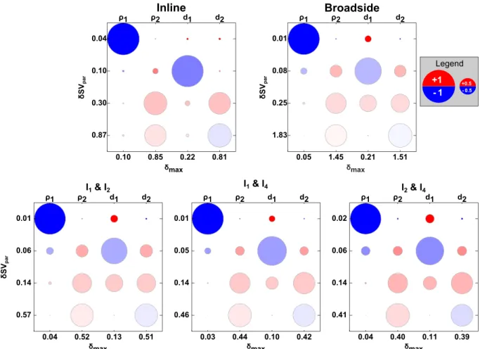
In Fig.6SVD-analyses are displayed for the scaled Jacobians of the pure inline and pure broadside responses (top row) and for scaled Jacobians of combinations of rotational invariants I1, I2and I4

(bottom row). We will explain the result and display of the analysis in detail for the inline response (top left-hand side):

The main axis displays the coefficients of the parameter matrix V^Twith circles of radii, which are proportional to the coefficients.

Positive and negative coefficients are shown as red and blue circles, respectively. Each row contains one SV-parameter and the displayed coefficients are the weights of the original model parameters within the according SV-parameter. The original model parameters are noted above the top axis. WithinV^T the SV-parameters are sorted with the most important, that is the one with the largest SV, located in the top row and least significant, that is the one with the smallest SV, being located in the bottom row. SV are normalized with respect to the largest SV and we use opacity along rows to show the importance of each SV-parameter: the top row with a normed SV of unity is completely opaque and rows 2–4 with SVs<1 become increasingly transparent. Please note that the SV is not explicitly noted in the plots. Instead we display the fractional standard error of each SV- parameter (δSVpar) along they-axis, which is simply the reciprocal of the SV. Estimates on the upper bound of the fractional errors of logarithmic model parameters (δmax) are given along the lower axis of the plot.

The first and second SV-parameters in the top two rows (Fig.6,

‘inline’) each have one dominant entry, which are associated with the model parametersρ1andd1. The fractional errors on the according model parameter areδmax(ρ1)=0.10 andδmax(d1)=0.22. Thus, the original model parametersρ1and d₁should be resolved better than±0.1m (=1m×0.10) and±22 m (=100 m×0.22). The third and fourth SV-parameter are no longer associated with a single model parameter, but rather combinations of model parametersρ2

andd2. Remembering that we have used log-scaling on the model parameters, we can use (11) for the 3rd SV-parameter:

(SVpar)≈V23·dlog (ρ2)+V43·dlog (d2). (17) Thus, the physical interpretation of this eigenparameter may be deduced as

ρ₂^V²³·d₂^V⁴³. (18)

(8)

Figure 6.Graphical display of SVD-analyses performed on scaled Jacobians, which contain the sensitivity for the CSEM configuration and 1-D model depicted in Fig.5(top panel: pure inline and pure broadside; bottom panel: combinations of rotational invariants I1, I2, I4). In each subplot, the radius of circles is proportional to the coefficients of matrixV^Tand positive and negative values are assigned the colours red and blue, respectively. Along each row the opacity of circles is scaled proportional to the corresponding singular value (SV). Because SVs are sorted and normed to the largest SV, the top row is completely opaque and transparency increases towards the bottom row. Along the y-axes we show the standard errors of the SV-parameters (SVpar), which is the reciprocal of the corresponding SV (Edwards1997). Along each bottomx-axis the estimates of the upper error bounds (δ^max) on the original parameters as calculated by eq. (12) are shown. The corresponding original model parameters are denoted along the topx-axis. Note that analyses are performed on log model-parameters as explained in the text.

Since both coefficientsV₂₃andV₄₃have the same sign, this is the resistivity-thickness product of the embedded resistive layer.

In a similar manner, the 4th SV-parameter contains the quotient of these model parameters, sinceV24andV44have opposite signs.

Generally speaking, the two model parameters could be resolved independently with the 3rd and 4th SV-parameter, provided the corresponding errors are small enough. However, for the inline response the according error estimates are close to unity [δmax(ρ2)= 0.85;δmax(d2)=0.81]. Thus, the assumptions made in the derivation by Edwards (1997) do not hold and the parameters cannot be considered to be resolved within the scope of the analysis performed here.

When comparing the inline response to the broadside response (Fig.6, top right-hand side) it becomes clear that the broadside response is less suitable to determine the model parameters. Ac- cording to the first SV-parameter,ρ1is resolved well (±0.05m), but the interdependence/mixing within the other SV-parameters is significant and the estimated upper error bounds on the parameters of the embedded layer are significantly higher. This is the reason why the radial/inline configuration is generally the preferred choice in detecting resistive structures (Constable2010).

Generally, for an experiment with two TX polarizations (Fig.2) all invariants can be calculated and may thus be jointly interpreted.

Therefore, we will compare the pure inline and broadside (Fig.6, top row) to combinations of two invariants (Fig.6, bottom row). Again, all analyses were based on the same basic 1-D model and geometry as depicted in Fig.5and measurement errors from the inline and broadside were propagated to the invariants via eq. (16). It is evident that the analyses of combinations of invariants significantly reduce the errors of the SV-parameters (δSVpar) and the upper error bounds of model parameters (δmax) as compared to the pure inline or pure broadside alone. The best resolution is given by combinations of invariants I₁and I₄(bottom middle) and invariants I₂and I₄(bottom right-hand side). For these invariants the upper error bounds of model parameters (δmax) are almost identical and absolute upper error bounds on the parameters are:

I1 and I4:ρ1 = ±0.03m, ρ2= ±2.22m, d1 = ±5 m, andd2= ±21 m,

I2and I4:ρ1 = ±0.04m, ρ2= ±2.00m, d1 = ±11 m, andd2= ±19.5 m.

As mentioned before, the results presented so far apply to the 1-D model and measurement geometry depicted in Fig.5as well

(9)

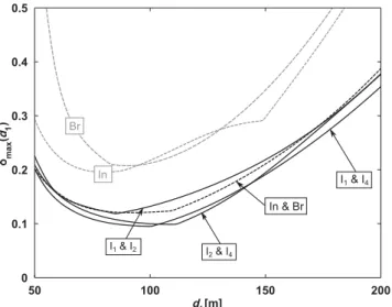
Figure 7.Fractional errorδmax(d1) for a varying thicknessd1of the model depicted in Fig.5. Errors derived from analyses of the inline (In) and the broadside (Br) responses and combined responses of invariants (I1, I2, I4), are depicted in grey and black, respectively. Also shown are the errors for the combined inline and broadside response (In and Br), which are similar to those of the combined invariants.

as the assumed standard error of measurements in eq. (15). To show that these results also apply in a broader sense, we have re- peated the analysis above for a whole set of models which are similar to the one depicted in Fig.5. The only parameter that is changed is d₁, which we vary between 50 and 200 m, which practically means that we shift the depth of the embedded resistive layer. The essence of this model study is contained in Fig.7, which shows the dependence of the fractional standard error for the model parameterd1

for the given model set. Dashed grey lines show the standard errors, which relate to analyses of the pure inline and the pure broadside (In and Br in Fig.7) and black solid lines the standard errors, which relate to analyses of combined rotational invariants (I₁and I₂, I₁and I4, I2and I4in Fig.7). It is immediately evident, that combinations of invariants always yield a better parameter resolution as compared to the pure inline or broadside. Looking at the combined invariants in detail, we see that combinations of invariants I1and I4and I2and I4yield similar error estimates over a wide range of models and usually perform better when compared to a combination of invariants I1and I2.

We have also included the results for the simultaneous analysis of inline and broadside responses (In and Br in Fig.7), for which the upper error bound is similar when compared to the combinations of two rotational invariants. This is to be expected, because for this study of sensitivities the rotational invariants are calculated from the inline and broadside responses using eq. (6). However, for a real measurement the rotational invariants offer the advantage to be determinable uniquely from any two, non-aligned transmitter polarizations, whereas the determination of radial and/or azimuthal components from two transmitter polarizations may not be unique, which poses a problem for the interpretation of data in terms of 1-D models.

Generally, the simultaneous interpretation of all three invariants is advisable for a real data set, but does not make sense in terms of the 1-D model studied here: for the 1-D case invariant I4depends solely on invariants I1and I2and is no longer independent, which can be seen by setting I3=0 in eq. (5).

In summary, the analyses of sensitivities demonstrate that measurements with two TX polarizations lead to significant improve-

ments in the resolution of 1-D layered structures. It seems evident that the use of more than one transmitter polarization will also help to improve the model resolution for 2-D or 3-D resistivity structures (see for example Newman et al.2010) and the concept of rotational invariants offers a convenient way to handle such data sets accordingly.

C A S E H I S T O RY

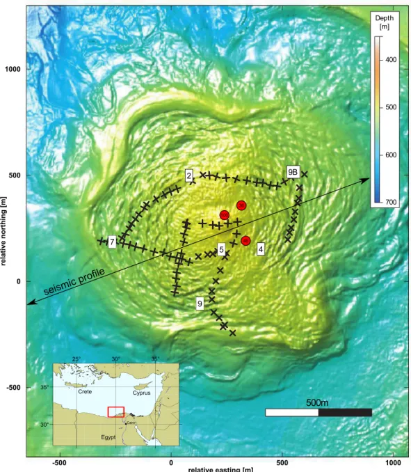
Geological setting of the North Alex Mud volcano The ‘North Alex’ mud volcano is located about 50 km to the North of Alexandria (Egypt) in the West Nile Delta (WND). The bathymetry of the central crest with a diameter of∼1 km is rather flat topped with water depths ranging between 500 and 515 m over the main crest (Fig.8). From previous remotely operated vehicle (ROV) dives it was known that ridges and troughs with a considerable relief of about 3 m exist at small scales (Dupreet al. 2007). They are visible as small scale, concentric undulations around the centre of the mud volcano in the bathymetric map. While the mud volcano was found in a relatively dormant stage with little activity during two research cruises in 2003 and 2004, active degassing and very high temperatures of almost 70^◦C at shallow depth of about 6 m were observed in 2008 (Fesekeret al.2010) during research cruise 64PE298 (R/V PELAGIA). During this research cruise, geophysical investigations (seismics and CSEM) were carried out to further investigate the internal structure of the mud volcano.

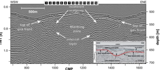
For the seismic experiment the source (105 in³GI gun) was towed 18 m behind the ship and operated with a shot interval of 7 s at a ship speed of three knots. Shots were recorded with a 100-m-long streamer with 32 channels. As an example, Fig. 9shows an fk- migrated (vp = 1500 m s⁻¹) CMP section, which was measured along a WSW–ENE striking profile across the centre of the mud volcano (Fig.8).

The seismic section in Fig.9shows a pull down of the main seismic reflectors to either side of the mud volcano (CMP 700–900 and 1500–1600). The fact that not all reffiectors are dipping to the same extent is not consistent with a pure velocity pull down effect, which should be similar for all reffiectors or increasing with depth. Therefore, the pull down reflects, at least to some degree, a structural deformation. The interior of the mud volcano is mainly characterized by blanking in the central part of the mud volcano (CMP 1100–1200 in Fig.9) and by incoherent scattering towards either side of this central part. Apart from the blanking and scattering, two prominent structural features are visible within the mud volcano:

The first marked feature in the seismic section (Fig.9) is a reflector directly beneath the seafloor. The reverse polarity of this reflector implies a negative impedance contrast and is interpreted to represent the top level of gas saturation within the mud volcano, since considerable degassing was observed around the centre of the mud volcano. Since theP-wave velocity decreases for gas saturations between 0 and 10 per cent and then remains consistently low for concentrations above this level (Minshullet al.2012), the reflector is indicative for the existence of gas but cannot yield quantitative estimates on saturation levels above 10 per cent.

The second feature, which is visible within the region of mostly incoherent scattering, is a reflector with normal polarity, which indicates an internal layer that can be interpolated to connect across the blanking zone to form a lens-shaped interface. According to the seismic section, this lens-shaped structure is approximately 1700 m

(10)

Figure 8. Bathymetic map of the North Alex mud volcano with locations of geoscientific investigations. The seismic section along the indicated profile is shown in Fig.9. White boxes and crosses show the locations of the CSEM receiver and transmitter stations, respectively. The actual systems are shown in Fig.10. Data samples from receiver 7 are shown in Fig.11. Red circles mark the locations of three gravity cores, for which porosities and resistivity logs were taken in laboratory measurements (Fig.17). Map after Fesekeret al.(2010), changed. Bathymetric data was provided courtesy of BP.

wide and has a vertical extent of∼0.18–0.2 s TWT with the base approximately between seismic CMP points 1125 and 1175 (Fig.9).

A remarkably similar section is described by Perez-Garciaet al.

(2009) for the H˚akan Mosby mud volcano (HMMV, see inlay in Fig. 9), which also show a pull down of reflectors towards the mud volcano, seismic blanking at and around the central conduit of the mud volcano and a lens-shaped feature centred beneath the mud volcano. At the HMMV the lens-shaped structure is slightly smaller with a lateral and vertical extent of∼1400 m and∼0.15–

0.16 s TWT, respectively, but the overall geometry is strikingly similar. Perez-Garciaet al.(2009) interpret the lens-shaped structure as collapse structure, which formed after the initial ‘birth’ phase of rapid mud volcanism. After a phase of inactivity the collapse structure was refilled in subsequent phases of mud volcanism. Thus, the reflector would represent an older, potentially more compacted

and cemented surface of the mud volcano from an earlier phase of active mud volcanism.

CSEM experiment

During the research cruise 64PE298 (R/V PELAGIA, 2008 Novem- ber) we had the possibility to use aCherokeeremotely operated vehicle (ROV) operated by the Ghent University (Belgium) for scientific experiments. The basic idea was to perform an experiment similar to the one described by Cairnset al.(1996) to investigate the resistivity structure of North Alex.

The main challenge for the successful implementation of a CSEM experiment similar to the one originally tried by Cairnset al.(1996) was to build a transmitter system with a sufficiently large dipole

(11)

Figure 9.CMP stacked and fk-migrated (Stolt1978) seismic section (v=1500 m s⁻¹) along the profile line indicated in Fig.8. For reference purposes, the numbering used for the CMP grid of the CSEM interpretation (compare Fig.12and Fig.14) is indicated above the section. The inlay on the lower right-hand side shows a seismic section from the H˚akan Mosby mud volcano (Fig.2a from Perez-Garciaet al.2009, changed) with a lens-shaped interface (red line), which is similar to the internal layer in the section from the North Alex mud volcano.

Figure 10.GEOMAR CSEM transmitter system and dipole antenna mounted to a Cherokee ROV (left-hand side). Nodal receivers (right-hand side) are deployed onto the seafloor to record the transmitted signals. The principal style of experiment is depicted in Fig.2, a station map of the CSEM experiment in the WND and data samples can be found in Figs8and11, respectively.

moment for the CSEM investigations at the mud volcano, which could still be handled by the smallCherokeeROV (size: 1.4 m× 0.9 m×1.2 m, weight: 450 kg, payload: <10 kg) which is very small compared to Alvin (size: 7.1 m×2.6 m×3.7 m, weight:

7 t, payload: 680 kg), which was used during the experiment by Cairnset al.(1996). The limited payload posed a first important constraint for the development of a TX system. As an additional restriction the available power supply from the ROV was limited to about 150 W. According to these limitations the transmitter was designed to be powered from a battery pack. With a capacity of 5 Ah (@42 V) the battery pack had enough power to transmit a signal of about 23.6 A into an electric dipole antenna for several min- utes. Since batteries were operated in a fast charging buffer mode, that is they were constantly recharged at an overvoltage of 52.5 V, they only needed about 1–2 min to recharge to full capacity after a

transmission cycles of up to 5 min. This was an acceptable compromise, since it was planned to only activate the transmitter with the ROV placed stationary onto the seafloor which left enough time for recharging while the ROV was to be moved from one station to the next. The transmitter (including the battery pack, dc–dc converters, H-bridge, electronics and a microcontroller unit, which allowed live control of the system using a RS232 serial interface) fit into a com- pact titanium pressure tube (Ø 160 mm, length 900 mm) with a negative buoyancy of about 10 kg in water. The pressure tube and floats, which compensated the weight of the pressure tube in water, were assembled in a small skid, which was mounted beneath the ROV (Fig.10, right-hand side). Furthermore, two sailing masts with stainless steel electrodes at their ends were mounted to the skid as dipole antenna with a total length of 9.1 m. The assembled system is shown in Fig.10(left-hand side). The ROV also carried

(12)

Rotational invariants for mCSEM data 235 a CTD probe, which constantly measured the conductivity of the

water column. The data acquired by this CTD probe compared well with conductivity data from two CTD casts, which were performed at the centre and at the edge of the mud volcano prior to the CSEM experiment. The CTD data showed no significant lateral or temporal variations and we have used this data to derive a layered conductivity model of the water column, which was used for the subsequent interpretation of CSEM data.

For the CSEM experiment we used five receivers (Fig.10, right- hand side), which were synchronized to GPS time prior and after the experiment. Each receiver is equipped with a three component fluxgate magnetometer, and can measure two components of the horizontal electric field. The components of the electric field are measured using Ag/AgCl-electrodes, which were attached at the end of four flexible arms. The total length of each receiver dipole is 10 m. Additional sensors allow measurements of the attitude (pitch, roll) and the temperature. The receivers can either be used in an MT- mode, in which all sensors are logged at sampling rates of up to 10 Hz, or switched into a CSEM-mode, in which only two components of the E-field are recorded at a high sampling rate of 10 kHz. This high frequency is necessary to acquire transient data at short offsets on the order of 100 m (compare Cairnset al.1996). The switch from one mode to the other can be performed by using a pre-set timetable or alternatively by an external acoustic signal. The receivers were deployed by free fall in an array onto the main crest ofNorth Alex (see Fig.8). One of the receivers (RX9) was recovered after the first ROV dive in the southeastern and central part of the mud volcano to check that the system was working correctly. After verification, it was redeployed to a new location (RX9B) northwest of the centre, where later measurements were scheduled. Before and after the CSEM experiment the receivers were operated in MT-mode. A comparison of the average total magnetic field values measured at receiver sites to the reference earth magnetic field of about 43 600 nT shows deviation of up to 1000 nT. Recent tests have shown that these deviations are mainly due to steady magnetic fields of releases (batteries, motor) and the influence of the steel anchor bars, which were used to connect the anchor weight to the release. Therefore, we have used the acquired magnetometer data to determine the heading of stations, but it is evident that these headings are biased to some degree. This bias could be mitigated by deriving a heading through coherency analysis of magnetic field variations at different rotation angles between stations and land observatory data. How- ever, in the context of this paper, where we rely on the analysis of rotational invariants, it is not relevant to pursue this issue further.

According to the receivers’ internal attitude sensors, the frames of all receiver stations came to rest in a stable position. For each receiver station, the final pitch and roll were below 8^◦with respect to the horizontal. The available video footage from the ROV also sug- gests that electrode arms were spread out straight onto the seafloor.

Measurements of the ambient noise floor yielded typical values of about 2×10^–8V/√

Hz. With the given transmitter dipole moment of∼215 Am and the receiver dipole length of 10 m this yields a noise floor of 10^–11V/(Am²√

Hz) for the source normalized E-field components.

The actual CSEM experiment was carried out during three ROV dives, which took place 4, 6 and 8 d after the deployment of receivers.

With the maneuverability of the ROV it was possible to operate the transmitter at a total of 80 locations (see Fig.8). At each location the transmitter was activated twice for 1 min with a bipolar, rectan- gular waveform (±23.4 A, 50 per cent duty-cycle, 0.25 Hz, ramp time<0.1 ms), once aligned and once perpendicular to the current profile direction. Thus, the measurement cycle for each transmit-

ter polarization contained 15 full switching cycles. The transmitter was placed at locations with a spacing of about 40 m on profile lines connecting the receiver locations. The ROV’s attitude sensors allowed an active control of the TX antenna’s orientation and tilt, which was less than 5^◦and 10^◦of the horizontal for 72 and 96 per cent of all measurements, respectively. For navigational purposes and the determination of distances, the ROV (carrying the TX) and four of the RXs were equipped with a GAPS (IXBLUE) acoustic positioning system. Depending on the signal-to-noise ratio, the accuracy of this system is stated to fall in a range between 0.2 and 1 per cent (@1σ) of the slant range (IXBLUE2012). With the given slant ranges of 600–700 m during our experiment, this amounts to an accuracy between 1.2 and 7 m (@1σ). This closely matches our observations, in which we found the accuracy of the system to be in the order of 5–8 m. The positions of receivers were also verified by video footage acquired with the ROV. RX4 was not equipped with a transponder and could not, due to shortage of time at the end of the experiment, be found during the last ROV dive. For this station we first used its drop position, which was then corrected by about 37 m to the NW using the approach described by Swidinsky & Edwards (2011).

The station map (Fig.8) shows the very different style of CSEM experiment with completely arbitrary TX and RX orientations which motivated us to use the previously introduced rotational invariants for the interpretation of the acquired data.

Data example

For processing the measured data sets for each transmission, each containing 15 full cycles (=1 min) of the transmitted bipolar waveform, were first cut into 15 segments. For each of these segments the measured half-cycles were averaged, which effectively removes the offset. The resulting 15 averaged half-cycles were then log-gated and stacked to yield step-on and step-off responses with corresponding error estimates for each logarithmic time step. We take the standard deviation of the stacking process as standard error of the measured data and use this error in the calculation of error bars for the rotational invariants.

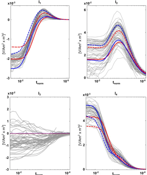
Fig.11shows invariants, which were calculated from the processed data at the westerly receiver RX7. For the sake of clarity, we only display TX–RX pairs with distances between 50 and 800 m, since clipping at short distances (∼50 m) and noise at long distances lead to significant distortions of the curves. The remaining 54 TX–RX pairs for this receiver yield invariants, which allow for a first-pass interpretation.

Red and blue lines in Fig.11show synthetic responses for homogeneous lower half-spaces of 0.7 and 1.3m, respectively. The upper section is represented by a 500 m thick, layered conductivity model derived from the CTD data, which is terminated by an infi- nite air half-space above. Since a finite water depth and the layered conductivity of the water column do have an effect on the invariants at longer offsets, the according synthetic responses are also plotted for the shortest (50 m, dashed) and longest offsets (800 m, solid).

For invariant I1 (Fig.11, top left-hand side) it can be seen that all measured invariants fall within the ‘corridor’ defined by these two synthetic half-space models. We have used this finding to derive an apparent resistivity transformation. In a companion paper by Swidinskyet al.(2015) we use this invariant to define an apparent resistivity transformation, which can be used for a fast imaging of CSEM data, which was measured with two separate TX polarizations. For I4and even more so for I2(Fig.11, right-hand side) it can

(13)

Figure 11.Rotational invariants calculated from real measurements (grey) recorded at receiver 7 on the North Alex Mud Volcano (Fig.8). Only TX-RX pairs with offsets between 50 and 800 m are displayed. Amplitudes of invariants are scaled by factors of r³(I1and I4) or r⁶(I2and I3), where r is the corresponding offset. Times are normalized as in Fig.4. Additionally, invariants of a 0.7m (red lines) and a 1.3m (blue lines) lower half-space are shown for offsets of 50 m (dashed lines) and 800 m (solid lines).

be seen that simple homogeneous half-space models cannot explain the curves. Thus, we will revert to 1-D inversions in the following chapter to investigate if rotational invariants can be explained rea- sonably well by a layered resistivity model of the subsurface with a significant increase of resistivity at greater depth. For the skew invariant I3 (Fig.11, bottom left-hand side) the responses of the half-space models are zero—as shown in the derivation of rotational invariants—but show significant amplitudes for the real data.

This could either be an indication for a 3-D resistivity structure, but might also be due to the partially non-planar geometry, bathymetric effects or a bias introduced by errors in the determination of

headings. Ultimately, a 3-D interpretation of the data will be necessary to distinguish possible causes and to fully explain all rotational invariants.

Common midpoint inversion of invariants

Since the experiment was not carried out along extended profiles but rather along many short subprofiles with changing orientations, we constructed a surface grid. For each cell of this grid we simultaneously inverted the data of all TX–RX combinations, whose

(14)

Figure 12. Common midpoint (CMP) grid with 75 m bins with the number of TX–RX combinations whose midpoints fall into the according grid cell indicated inside each cell. The according TX–RX combinations of each CMP cell were simultaneously inverted for in regularized 1D smooth inversions. The colour of cells depict the achieved rms misfit. Labels in black boxes are used to identify CMP cells or profiles in the text. For reference purposes, the locations of receiver stations (white boxes) and of the seismic line are also shown. Map after Fesekeret al.(2010), changed.

midpoints fall into the respective grid cell, in terms of a 1-D layered model. To achieve a good compromise between lateral resolution and a grid without too many empty cells, we chose a grid spacing of 75 m.

In Sommeret al.(2013) we have investigated the effects of the bathymetry for the WND data set. There, we have found that at short TX–RX offsets there can be a significant difference (in terms of theχ²-misfit) between the transient response of an assumed planar measurement geometry as compared to the response of the true, non- planar measurement geometry (including bathymetry). Especially for TX–RX pairs with offsets of less than 125 m we frequently observed χ²-misfit above 1. Consequently, we have rejected all offsets of less than 125 m for the CMP inversion. The assumption of a planar geometry also does not hold, if either transmitter or receiver show a significant tilt. This was the case at some locations, where

ridges and troughs formed considerable relief. Therefore, invariants which contain at least one TX polarization with tilt≥10^◦were also rejected. The resulting common midpoint (CMP) coverage for the 75 m bins after rejection of data sets with respect to short offset or excessive tilt is shown in Fig.12(white labels).

For the data interpretation we used a constrained regularized 1-D smooth inversion (Constableet al.1987) based on the Matlab functionlsqnonlin, which is contained in the Optimization Toolbox (Coleman & Li 1994, 1996). For each CMP cell we invert for the resistivities of a multilayered 1-D model. In a 3-D case study, Constable (2010) demonstrated that the marine CSEM method over a 1m half-space is not sensitive to any structure deeper than or offset by more than about half the source–receiver spacing, which closely matches our experiences. Consequently, for our inversion the depth of the last layer interface is set to 45 per cent of the