A binary logistic analysis of car consumer behavior in China

Humboldt-Universität zu Berlin

Institute for Statistics and Econometrics

A Binary Logistic Analysis of Car Consumer Behavior in China

Bachelor Thesis Bachelor of Science

Study of Statistics August, 22, 2006

Presented by: Shen Guan (184728) Tester: Prof. Dr. B. Rönz

Email: cerbrinags@hotmail.com

AUTHORSHIP DECLARATION

I hereby declare and confirm that this thesis is entirely the result of my own work except where otherwise indicated. I have acknowledged the supervision and guidance I have received from Professor Bernd RÖNZ.

Shen GUAN

22 /August /2006

ACKNOWLEDGMENT

I hereby acknowledge Professor Bernd RÖNZ for his supervision, guidance, availability and friendly support during my work on this thesis. I also appreciate the guidance and help from Szymon Borak.

I am very grateful to my family and my dear friend Sonia

Boyum for their encouragement and support.

Contents

1. Introduction……….1

2. Background: Today’s Chinese car market………....5

3. General Data Overview………..7

I. Data Source………7

II. Choice of Variables………..8

4. Logit Model ………..13

5. Stepwise Backward Elimination and Bivariate Analysis….16

6. The fit of the model………..20

7. Interpretation of the model ………22

8. Some Discussions about Chinese Auto market ………25

I. Second-Hand Auto market ………....25

II. Financing in Chinese Auto market………...27

Appendix……….30

References………...33

List of Figures

Figure 2.1: Car Unit Profitability in China (in US dollars)………...6

Figure 2.2: Chinese passenger car and light vehicle sales in period 1993 to 2002 ....………....6

Figure 3.1: Not Buy vs. Buy ………9

Figure 3.2: Distribution of Gender ………....10

Figure 3.3: Distribution of Age.……….10

Figure 3.4: Distribution of Education..………...11

Figure 3.5: Distribution of Income……….11

Figure 3.6: Distribution of Occupation..……….11

Figure 3.7: Distribution of Family Size………..12

Figure 5.1: Decision vs. Income……….19

List of Tables Table 2.1: Market share of Auto makers’ Market share ………..5

Table 3.1: Variable List ………...8

Table 5.1 Forward Stepwise with Wald ……….17

Table 5.2: Pearson’s Chi-Square Significance Test ………...18

Table 7.1: Logit Model done with subcategories..………..24

Table 8.1: Distribution of Payment……….27

Table 8.2 Divided Payment vs. Full Payment……….28

1. Introduction

China’s entry into the World Trade Organization (WTO) in December 2001 opened the market to foreign competition and triggered a surge in foreign direct investment.

Consequently, automobile tariffs declined and thus caused a price drop in the overall Chinese automobile market. It was assumed that the demand for cars would be stimulated as a result, which would drive the car market to grow rapidly.

From December 2001 to 2002, a growth in sales described as “gushing sales”

brought by the accession into the WTO can be read from the following data: total vehicle sales reached 3.38 million in 2002 (up 1 million from 2001), a surge of 37%.

Over 80% of the individual car buyers purchased a car for the first time. (Shanghai Stock Newspaper, Jan. 23, 2003). There is a small group of Chinese who are younger, better educated, more urbanized and have a higher income that are typically considered as the middle class segment and leaders in the Chinese consumption market. Many already possessed a car before China’s entry into the WTO. On one hand, although the car price fell as a result of WTO-accession, the relationship between private income and car price is still to a great degree disproportional. It might still be a heavy financing burden for the middle class Chinese people to replace their cars or own a second one. On the other hand, simultaneously, some new benefits other than price cutting brought by WTO would generate new characters of the consumer behavior of car buyers. New rules and possibilities affect not only the people who decide to buy a car for the first time, but also those who have already owned cars. Various choices for car brands and modern car designs, integrated after-sale-services, professional and advanced financing means, etc., would effectively attract car owners to purchase a second automobile.

This paper analyzes the probabilities of the car owners of replacing or buying a second car and the factors that influence their decisions by using the logit model performed in SPSS 13.0.

2. Background: Today’s Chinese car market

China is the fourth largest and the fastest growing car market in the world.

Moreover, high unit profitability of cars and Chinese consumers’ continually booming demand for motor vehicles have made China a huge potential car market for many carmakers, especially considering the 1.3-billion population of this country.

In the last few years, some profound developments, such as China’s entry into the WTO, have greatly accelerated the pace of Chinese car market growth. The foreign car producers, who have taken the “first move” years earlier, still dominate the market with considerable market shares (Table 2.1) and make very high profit per unit (Figure 2.1). VW for instance, enjoyed huge “first mover” advantage (approx.

1985) of large market share, selling close to 500,000 passenger cars in China in 2002 at a high profit.

Source: China Association of Automobile Manufacturers.

Table 2.1 Market share of Auto makers’ Market share

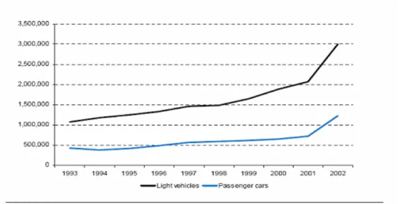
As showed in Figure 2.2, Chinese passenger car and light vehicle sales in the period from 1993 to 2002 grew rapidly, especially from December 2001, the time of China’s entry into WTO, to 2002. For many years, government officials and

corporate customers were the main car buyers, but the recent rate of acceleration can only be explained by a large surge in purchases by private individuals. In Shanghai for example, private vehicle registrations were 7,000 in 1998, 83,700 in 2001, and 167,000 in June 2003.

Source: Company data, Goldman Sachs Research estimates.

Figure 2.1 Car Unit Profitability in China (in US dollars)

Figure 2.2 Chinese passenger car and light vehicle sales in period 1993 to 2002

3. General Data Overview

I. Data Source

The data used in this paper comes from a survey done by Beijing Kangkai Controlling Company in cooperation with National Bureau of Statistics of China in August 2001, about three months before China’s entry into WTO. The entry into the WTO would definitely increase the accessions of foreign enterprises into Chinese market, which would strengthen the market competition and thus put enormous pressure on Chinese state-owned enterprises. After a long period of time of planned economy, the WTO membership means more chances and also larger challenge for those enterprises. This survey was done to help the Chinese state-owned auto manufacturers to work out a proper marketing strategy to face the market change.

It included four parts: i. External situation for car using (air quality, oil supply, parking possibilities, etc.); ii. Self-evaluation of consumption behavior and psychology; iii. Consumer car purchasing behavior; iv. Plans for buying a new car in the next 5 years, which tried to:

◆ analyze the consumer behavior of the current car owners;

◆ find out the attributes of private individual demand for cars;

◆ find out the various influences on car demand;

◆ research and define a proper car price suitable for Chinese market;

◆ forecast the development of the Chinese car market in 5 years.

It was done in 38 cities, each city included 218 interviewees and three limitations were set on the interviewees:

◆ yearly income: over 30,000 RMB¹;

◆ age: between 20 to 55 years;

◆ car ownership: yes.

1 Change rate in 2001: 1$= 8.277RMB in average. (data source: State administration of foreign exchange, China).

More explanations are necessary to the first limitation. According to the analysis of international car market, most individuals have the ability to purchase a new car when the GDP per capita reaches $3000, i.e., 3000$ is the boundary to financing ability for purchasing a new car. In 2003, although the GDP per capita in China is

$900, but in some well developed cities, especially in some east coast cities (Appendix 1), the GDP per capita level has already exceeded 3000$, i.e., there is a large group of people who have the financing ability to buy cars (Data source:

Beijing Auto, The currency and development of Chinese car market, Page20, February 2003). The financing boundary to those who want to own a second car may be higher, so it makes sense to set a higher income limitation of 30,000 RMB which is equal to $3625 on the interviewees.

II. Choice of Variables

Only the data from 7 cities which cover 1526 interviewees would be analyzed, since it is not necessary to do the analysis of all the 38 cities due to the enormous amount and also the repetition of the data.

The variables (Table 3.1) from the last two parts of the survey “consumer car purchasing behavior” and “plans for buying a new car in the next 5 years” are picked out because of the objectives of this paper.

Table 3.1 Variable List

i). The dependent variable

Decision is a binary variable with two categories not buy and buy. The question was:

do you plan to replace your car or to buy a second one in next 5 years? The answers were: a) yes, very sure; b) maybe yes; c）maybe not; d) definitely not; e) I do not know yet. In order to satisfy the conditions of Logit Model, the answers are classified into two groups: a) yes, I plan to buy a car; b) no, I do not plan to buy a car. The answers “a” or “b” are classified into the category buy and answers “c” or

“d” into the category not buy. Answer “e” with the weight in whole sample 10.3% is defined as missing value (appendix 1). The valid percent for not buy is 54.4% and buy 45.6%.

buy not buy

60.0%

50.0%

40.0%

30.0%

20.0%

10.0%

0.0%

Figure 3.1 Not Buy vs. Buy

ii). The independent variables

Six variables are chosen from the survey as independent variables. Basic descriptions to the characteristic of each variable are showed as followed.

City: Beijing, Shanghai, Tianjin, Nanjing, Hangzhou, Fuzhou, Guangzhou and each city includes 218 interviewees (Appendix 2). Compared to other cities in China, these 7 cities are more developed and considered to be more sensitive to market changes; higher living standard enables their residents to pay for new designs and fashions. Additionally, those cities are geographically distributed from north to south across China, i.e. the analysis by using the data from these cities would well

represent the fluctuations and differentiations of car consumption in different regions.

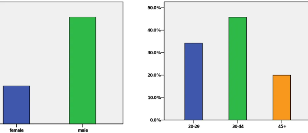
Gender. 73.8% of the valid responses, which is 1123 observations, are male and 26.2% of the valid responses, in amount of 399, are female. The fact that most car owners in China are male results in the proportion of male car ownership about 3 times higher than female (Figure 3.2).

Age. In order to guarantee that every subcategory has enough observations, this variable is re-classified into 3 categories. The group 20-29 is 34.2% in the whole sample, which has 521 valid observations and the group 30-44 has 697 observations with the weight of 45.8%. The oldest group of 304 observations is only 20% of the whole sample, since auto is a relative modern household consumption in China and therefore more young people own cars than old people (Figure 3.3).

45+

30-44 20-29

50.0%

40.0%

30.0%

20.0%

10.0%

0.0%

Figure 3.2 Distribution of Gender Figure 3.3 Distribution of Age

male female

80.0%

60.0%

40.0%

20.0%

0.0%

Education. This variable is re-classified into 2 categories “attended university” and

“did not attend university” (in short: not attend uni and attend uni). The sub- category not attend uni has 680 observations equal to 44.6% of total interviewees and attended uni 844 observations equal to 55.4% of the whole sample. 1524 observations are valid for this variable. There are enough observations in each subgroup for analysis. As showed, the proportion of auto ownership for those people who have a university degree is lightly higher than those who without (Figure 3.4).

Income. This variable is re-classified from 12 categories into 3 categories: 2500- 3500 RMB, 3501-5000 RMB, more than 5000 RMB. The category “declined to answer” which has 127 observations is defined as missing values in this paper. So the valid observation for this variable is 91.7% of the whole sample. The sub- category 2500-3500 RMB has 696 observations which is 49.7 % of the valid sample, and 3501-5000 RMB 276 observations equal to 19.8% of the valid sample, 5001+

RMB has 427 observations equal to 30.5% (Figure 3.5).

attend uni

Figure 3.4 Distribution of Education Figure 3.5 Distribution of Income

Occupation. This variable is re-classified from 13 categories into 4 categories.

There are 350 observations in the sub-category Government service equal to 23% of the whole sample and Employer 444 observations equal to 29%, Employee 370 equal to 24.3%, Others (including student, retired and other occupations) 361 observations equal to 23.7% (Figure 3.6).

Figure 3.6 Distribution of Occupation

not attend uni 2500-3500RMB 3501-5000RMB 5001RMB +

50.0%

40.0%

30.0%

20.0%

10.0%

0.0%

60.0%

50.0%

40.0%

30.0%

20.0%

10.0%

0.0%

others employee

employer government

service 30.0%

25.0%

20.0%

15.0%

10.0%

5.0%

0.0%

Family Size. The question for this variable was: what is the number of family members? This variable is re-classified from 6 categories into 3 categories: 1 or 2 persons, 3 persons, 4 persons or more. The first group has 192 observations equal to 12.6% of the whole sample and the second group 925 observations equal to 60.8%, the last group 405 observations equal to 26.6%, respectively. As seen, the sub-group 3 persons has an overwhelming majority due to the Chinese one child policy (Figure 3.7).

4 persons or more 3 persons

1 or 2 persons 70.0%

60.0%

50.0%

40.0%

30.0%

20.0%

10.0%

0.0%

Figure 3.7 Distribution of Family Size

Accumulated Mileage. This variable is a numeric variable and the question was:

what is the accumulated mileage of your car. According to the survey, 80% of the private owned autos were bought after 1998 and only 17.6% of autos are second hand. Moreover, the mean value of Accumulated Mileage is ca. 95,000 kilometers, that is, the average condition of the autos is quite well, which may lead to the percentage of “not buy” in the dependent variable is appreciably higher than that of

“buy”. Additionally, because a car is still a luxury item for most Chinese families, Accumulated mileage should play a big role in the decision to replace a car. In next chapters, this answer would be tried to find out if Accumulated Mileage has significant influence on the dependent variable or not.

4. Logit Model

In many applications, logistic regression is a standard method for explaining a binary dependent variable that has two categories equal to either 1 or 0 partly because of its mathematical convenience. Logistic regression is different from linear regression, but there are many similarities. Concepts from linear regression would be carried over to logistic regression.

Under the assumption that a set of independent variables x are included in the model, then the dependent variable y can be described as a linear combination of the independent variables x and the parameters β plus the error term ε , in form as:

y_i =x_i^Tβ +ε_i =β₀ +β₁x_i1+...+β_jx_ij +ε_i (4.1) The linear regression consists of two parts: the mean value of the outcome variable

that can be expressed as a linear function of the independent (predictor) variable and the error that attempts to describe how individual measurements vary around the mean value. It is assumed that individual responses vary around the mean according to a normal distribution with varianceσ². This model can be expressed as:

·Structure on the means: E(Y_i X_i)=β₀+β₁x_i1+...+β_jx_ij (4.2)

·Error structure: ε_i ~N(0,σ²) (4.3) For a binary response variable, we assume that prob(Y_i =1)=π_i , so we have

i

Yi

prob( =0)=1−π , in general we then have:

i i i

Yi

E( )=0×(1−π )+1×π =π (4.4) The expression (4.2) implies that is possible for the quantity E(Y_i X_i) to take on any value as x ranges from −∞ to +∞. If the dependent variable is a binomial, this quantity is constrained to [0,1], which can be seen in (4.4).

The binary nature of the response also creates difficulties in how we view the variability of individual values around the mean. The variance of a binary response

is a function of the probabilityπ_i, which is:

) 1 ( )

(Y_{i i i}

Var =π −π (4.5) The quantity Var(Y_i)is the function of π_i, i.e., the assumption constant variance

is violated. So the linear regression is not proper for a binary response variable.

σ2

The quantity π_i =E(Y_i X_i)is used for logistic distribution in order to simplify notation, and we have:

(4.6)

i

yi

y e

F =

= ( )

π

_{i i y}

+ e 1

With y_i =x_i^Tβ =β₀+β₁x_i1+...+β_jx_ij

There is a very important property about function (4.6) that makes it proper to build up a model for binary dependent variable, that is, (4.6) is bounded between 0 and 1.

This will eliminate the possibility of getting nonsensical predictions of proportions or probabilities.

From (4.6) we get:

^{y i}

i

i = e

−

π π

1

(4.7)

i

π

i

π

−

1

is called odds which represents the relationship between the probabilities that dependent variable Y takes the outcome of 1 comparing to the outcome of 0, and odds can also take any positive value and therefore have no ceiling restriction.

Moreover, there is a linear model hidden in (4.6) that can be revealed with a proper transformation of the response. This transformation called logit transformation that converts the probability into a continuous variable that is linear with respect to

the explanatory (independent) variables (McCullagh and Nelder 1991) is defined in terms of π_i as followed:

_i^T _{i j ij}

i i

i X x x

y β β β β

π

π = = + + +

= − ) ...

log(1 _{0 1 1} (4.8) From (8) we can see, y_i is exact the logarithms of

i

πi

π

−

1 in form as

1 ) log(

i i

π π

− also called as logit or log-odds.

In linear regression, the least squares method (LS) is most often use to estimate parameters. But the least-squares regression approach is plagued with many statistical problems for logit model, so the maximum-likelihood (ML) fitting procedure is most frequently used (Hosmer and Lemeshow 1989). In general, the ML technique is used to maximize the log-likelihood function, which indicates how likely it is to obtain the observed values of Y, given the values of the independent variables and parameters (Menard 1995).

5. Stepwise Backward Elimination and Bivariate Analysis

This chapter is about testing of a statistical hypothesis to determine whether the independent variables included in the model are significantly associated with the response variable.

Stepwise logistic regression, which offers a fast and effective means of screening a large number of variables, and simultaneously fit a number of logistic regression equations, is most often used in situations were the “important” independent variables are not known and associations with the outcome not well understood (Hosmer and Lemeshow 1989).

There are two basic forms of stepwise logistic regression: forward inclusion and backward elimination. Backward elimination, more exact, backward elimination of Wald is used in this paper. In backward stepwise elimination, the analysis begins with a model that contains all of the explanatory variables. At each step, the significance of the explanatory variable being removed is tested using the Wald test² (Hosmer and Lemeshow 2000; Duncan and Chapman 2003). If a variables p- value is equal to or greater than the significant level, it will be eliminated from the model, otherwise, it remains in the model. As a result, the final model consists entirely of variables that are statistically significant (Hosmer and Lemeshow 2000).

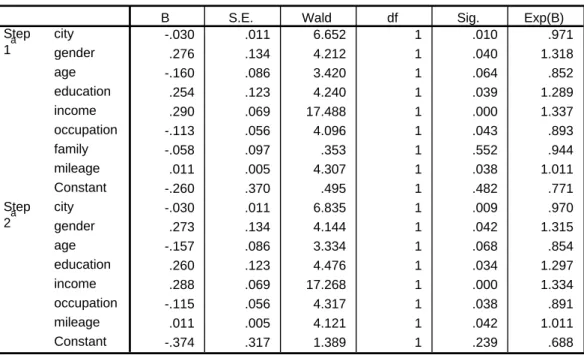
Table (5.1) shows the SPSS output of forward stepwise with Wald. The model includes all the explanatory variables at the first step and we can see, the p-value of Family Size is 0.552 that is much large than the significant level, which indicates

2 The Wald statistic

ˆ ) ˆ(

ˆj

W σ β

= β

j

follow a chi-square distribution and in this case, with one degree of

freedom.

that Family should be removed from the model, which is also showed in step 2.

Variables in the Equation

-.030 .011 6.652 1 .010 .971

.276 .134 4.212 1 .040 1.318

-.160 .086 3.420 1 .064 .852

.254 .123 4.240 1 .039 1.289

.290 .069 17.488 1 .000 1.337

-.113 .056 4.096 1 .043 .893

-.058 .097 .353 1 .552 .944

.011 .005 4.307 1 .038 1.011

-.260 .370 .495 1 .482 .771

-.030 .011 6.835 1 .009 .970

.273 .134 4.144 1 .042 1.315

-.157 .086 3.334 1 .068 .854

.260 .123 4.476 1 .034 1.297

.288 .069 17.268 1 .000 1.334

-.115 .056 4.317 1 .038 .891

.011 .005 4.121 1 .042 1.011

-.374 .317 1.389 1 .239 .688

city gender age education income occupation family mileage Constant Step

1^a

city gender age education income occupation mileage Constant Step

2^a

B S.E. Wald df Sig. Exp(B)

Variable(s) entered on step 1: city, gender, age, education, income, occupation, family, mileage.

a.

Table 5.1 Forward Stepwise with Wald

But, the model should not totally be based on the results of the Wald test. Hauck and Donner (1977) found out that the Wald test behaves in an aberrant manner, often failing to reject the null hypothesis when the coefficient is significant. They suggested that the likelihood ratio test should be used for the logit model. For large sample size, there is practically no difference between the results of the likelihood ratio test and Pearson's chi-square test (Rönz 2000). In the next step, Pearson's chi- square test would be used to find out if there any more variable except Family should be excluded from the model.

Pearson's chi-square is by far the most common type of chi-square significance test.

This statistic is used to test the hypothesis of no association of columns and rows in contingency table. In the binary analysis in this paper, the association between response variable Decision and every other variable (except Family) is tried to find out based on binary contingency tables. Pearson's chi-square test is not appropriate

for the continuous variable, out of convenience, Accumulated Mileage is turned from a continue variable into a categorical one by dividing it into 2 groups: under and over the average value 95,000 kilometers. Since this classification has ensured that each subgroup has enough samples to satisfy the condition of Pearson's chi- square test, other classifications would not be tried (Appendix 3). If the p-value of the tested variable is larger than the significant level, the hypothesis would be rejected, that is, this variable should be eliminated from the model.

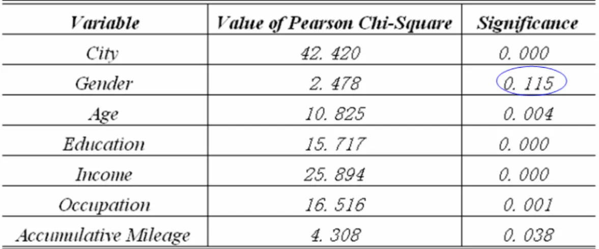
Table (5.2) indicates that at 5% significant level, every independent variable is related to the response variable except Gender, meanwhile, City, Education and Income are statistically the most significant ones with p=0. According to the suggestion of Hosmer und Lemeshow (1989), if the p-value in Pearson's chi-square significance test is smaller than 0.25, i.e., the variable may have in some sense weak effect on the outcome variable, and then it should not be eliminated from the model.

So, although the Gender is not significant, it still remains in the model.

Table 5.2 Pearson’s Chi-Square Significance Test

From Table (5.2) we can see that Income is the one of the variables that has is strongly associated with the outcome variable Decision. In China, more and more individuals plan to buy a car, but the disproportionately high cost of new cars compared to individual wealth makes it difficult for consumers to afford, especially

a the second purchase. Income is assumed to be the key factor that influents the decision of “buy” or “not buy”. Figure (5.3) shows us that for the group 2500- 3500RMB, the percentage for “not buy” is higher than that of “buy”, for the group 3501-5000RMB, the percentage for “buy” precedes that of “not buy”, even though the difference is not that significant. For the third group 5001RMB+, this difference is even greater with a bigger margin. This result also confirms the presumption that the correlation between Income and Decision should be strong (Figure 5.1).

5001RMB + 3501-5000RMB

2500-3500RMB 60.0%

50.0%

40.0%

30.0%

20.0%

10.0%

0.0%

buy not buy decision

Figure 5.1 Decision vs. Income

6. The fit of the model

The fit of the model was tested after the elimination to ensure that the model adequately fits the data.

As mentioned earlier, the Maximum-likelihood-method would be used to estimate the parameters β in the logistic regression. For the binomial distributed response variable y we have the likelihood function as followed:

i i

i n y

i y i i i i

i y

y n

L ⎟⎟ − ⁻

⎠

⎜⎜ ⎞

⎝

=⎛ (1 )

)

;

(π π π (6.1) Taking the log of (6.1), we get:

⎟⎟⎠

⎜⎜ ⎞

⎝ + ⎛

−

⎟⎟+

⎠

⎜⎜ ⎞

⎝

⎛

= −

i i i

i i i i

i

i y

n n y

y

l log(1 ) log

log 1 )

;

( π

π

π π (6.2)

So the joint likelihood-function is:

∑

∑

^⎥

⎦

⎢ ⎤

⎣

⎡ ⎟⎟

⎠

⎜⎜ ⎞

⎝ + ⎛

−

⎟⎟+

⎠

⎜⎜ ⎞

⎝

⎛

= −

=

i i

i i

i i i i

i

i

i y

n n y

y l y

l log(1 ) log

log 1 )

; ( )

;

( π

π π π

π (6.3)

Deviance in notation of D is an important statistic in some approaches to assessment of goodness-of-fit, defined as:

[

(ˆ ; ) (ˆ; )

]

~ ²( 1)

) 2 ˆ ; (

)

; ˆ log (

2 = − _{− +}

−

= _{sat i j}

sat

y l y y l

l y

D l π π χ

π

π (6.4)

) ˆ; ( y

l π : likelihood of the current model )

ˆ ;

( y

l π_sat : likelihood of the saturated model³ )

,...., ,

( _{1 2}

'

yi

y y y =

) ,...., ,

( _{1 2}

'

xj

x x x =

The role of deviance in logistic regression is as same as SSE (residual sum-of- squares) in linear regression. Actually, deviance is exactly equal to SSE when

3 Saturated model is one that contains as many parameters as there are data points. The log-likelihood-function for the saturated model is:

∑

^⎥

⎦

⎢ ⎤

⎣

⎡ ⎟⎟⎠

⎜⎜ ⎞

⎝ + ⎛

⎟⎟⎠

⎜⎜ ⎞

⎝

⎛ −

−

⎟⎟+

⎠

⎜⎜ ⎞

⎝

= ⎛

i i

i i

i i

i i i i

sat y

n n

y y n n

y y y

l(πˆ ; ) log ( )log 1 log

computed for linear regression.

Now we assume is the deviance for the model which has a set of independent variable , analog, is the deviance for the model

which has a set of independent variable , then and are nested models. The statistic

D0 M₀

) ,...., ,

( _{1 2}

'

xj

x x

x = D₁

M1 x^' =(x₁,x₂,....,x_j+p) M₀

M1 ΔD, also refer to as the “likelihood ratio test”, would be applied to answer the question “Does the model with the variable give us more information about the response variable than that without the variable”. It is a close analogue to the F statistic for linear regression.

[

(ˆ ; ) (ˆ; )

] [

2 ( ; ) (ˆ; )

] [

2 (ˆ; ) (ˆ; )

]

2 _{0 1 1 0}

1

0 D l y l y l y l y l y l y

D

D= − = π_sat − π − π_sat − π = π − π

Δ (6.5)

The degrees of freedom of ΔD is:

(degrees of freedom of M₀) – (degrees of freedom of M₁)

=

[

^i−(j+1)

] [

^{− i−(j+ p+1)}

]

^{= p}

Since D₀ and D₁ are both χ² -distributed, ΔD is also -distributed with p degrees of freedom. If the p-value exceeds the significant level, it is concluded that the reduced model is as good as the full model.

χ2

The SPSS statistical package presents not the log-likelihood itself but the log- likelihood multiplied by –2 (SPSS Inc. 1998). Output from SPSS denotes log- likelihood multiplied by -2 as “-2 Log Likelihood” (Appendix 4). By multiplying the log-likelihood by -2 it approximates a chi-square distribution (Menard 1995). As showed in chapter 5, Family Size should be excluded from the model. Now ΔD would be calculated to compare the two models with and without Family Size to see the goodness-of-fit of the reduced model:

=

ΔD 2[likelihood of full model - likelihood of reduced model]

= 1668.365 – 1665.007= 3.358 (6.6) In this case, the freedom of degree of ΔD is 1, since only one variable is removed from the model. The statistic value (6.6) is larger than the critical value at 10%

significant level equal to 2.71, demonstrating that Family Size adds little to the model once the other variables have been taken into the model.

7. Interpretation of the model

The independent variables, except Accumulated Mileage, are categorical variables.

These variables would be analyzed as a series of indicator variables to correctly evaluate their importance in the model. For the variable with k categories, indicator variables must be constructed. In the data, for example, Education has two categories, not attend uni and attend uni, and needed only one indicator variable.

Meanwhile, Income has 3 categories and therefore two indicator variables are necessary for our analysis of this independent variable. Here, every first category of the categorical dependent variables is taken as the reference category (Appendix 5).

−1 k

Table 7.1 shows us how important the other categories of the categorical variables are to the outcome variable.

Since Gender is not significant to 5% with p-value 0.113, the program proceeds to the second step. Gender is removed from the model in the second step, which is consistent with the result of Pearson's chi-square significance test (see Table 5.2).

In the second step we can see, City has significant influence to response variable Decision at 5% significance level, but in the subcategories, only Shanghai and Fuzhou are significant. The independent variable has no influence on the response variable if the odds ratio, which is presented in SPSS as Exp (B),equals to 1. The larger the difference is between the observed odds ratio and 1.0, the stronger the relationship is. Here, the odds ratio of 1.6 indicates a moderate relationship.

According to the odds ratios, we also can say, for those who live in Shanghai, the probability of planning to purchase a second car in next 5 years is about 1.6 times higher than in Beijing. So, only based on the decision to purchase a second car, the automobile market in Shanghai has more potential compared to Beijing. Meanwhile, those in Fuzhou are 33% less likely to plan to buy another car than those in Beijing.

The p-value of Age is 0.013, which results to the conclusion that it is strongly associated with the outcome variable Decision. Broadly speaking, younger people

show stronger desire to purchase a second auto compared to older people. The age group 30-44 is not significant, with a p-value equal to 0.180, which exceeds the critical p-value (α =0.1). The age group 45+ is about 58.6% less likely to answer yes to “do you plan to renew your car in next 5 years” when compared to the age group 20-29.

Education shows also significance to the response variable with a p-value equal to 0.021. The group with a university degree is about 1.35 times more likely to plan a second auto purchase than the group without one.

Income plays a very important role in consumer decisions. It is also confirmed to be true according to the analysis that the p-value of Income is 0, that is, Income is one of the two variables that are most significant to the outcome variable. In this variable, both subgroups 3501-5000 and 5001+ are strongly associated with Decision. The result shows us that the probability for the group with income of 3501-5000RMB is 1.38 higher than the group with lower income of 2500-3500RMB considering the second auto purchase. And the probability for group 5001+RMB is 1.82 times higher than that for group 2500-3500RMB.

The association between Occupation and Decision is strong as it can be seen from the p-value equal to 0.014, but only one subcategory employer of this variable is significant. From the value of Exp(B), it is concluded that the probability for employer to replace their cars is 1.32 times more than the people who work for government.

As showed, the p-value of Accumulated Mileage equals to 0.006, which confirms the presumption that this variable should have significant influence on the dependent variable. The coefficient of Accumulated Mileage is 0.015, the odds ratio Exp (b) is equivalently equal to 1.015 as showed in the output. An odds ratio above 1 indicates an increase, in this case, the odds ratio equals to 1.015, it is said that when the Accumulated Mileage increases one unit, the odds that the dependent = 1 increase by a factor of 1.015 when other variables are controlled, i.e., the probability to purchase a second car would increase 1.5%.

The analysis shows that the variables City, Age, Education, Income, Occupation and Accumulated Mileage have influence on the dependent variable. General speaking, those who are younger, better educated and have higher income are more likely to have a second car in next 5 years.

Variables in the Equation

49.413 6 .000

.472 .222 4.539 1 .033 1.604

-.276 .220 1.574 1 .210 .758

-1.110 .228 23.802 1 .000 .330

-.034 .234 .021 1 .886 .967

-.211 .214 .971 1 .324 .810

-.272 .247 1.208 1 .272 .762

.219 .138 2.518 1 .113 1.245

9.221 2 .010

-.210 .146 2.075 1 .150 .811

-.555 .183 9.190 1 .002 .574

.305 .131 5.470 1 .019 1.357

14.817 2 .001

.312 .162 3.723 1 .054 1.366

.579 .152 14.590 1 .000 1.784

9.783 3 .021

.280 .173 2.641 1 .104 1.324

-.204 .180 1.281 1 .258 .815

-.156 .181 .741 1 .389 .856

.015 .005 7.764 1 .005 1.015

-.493 .265 3.450 1 .063 .611

49.327 6 .000

.473 .221 4.552 1 .033 1.604

-.292 .220 1.762 1 .184 .747

-1.106 .227 23.667 1 .000 .331

-.036 .234 .024 1 .877 .965

-.184 .213 .744 1 .388 .832

-.243 .246 .976 1 .323 .784

8.634 2 .013

-.195 .145 1.797 1 .180 .823

-.534 .182 8.584 1 .003 .586

.301 .130 5.314 1 .021 1.351

15.904 2 .000

.319 .162 3.887 1 .049 1.375

.598 .151 15.686 1 .000 1.819

10.571 3 .014

.294 .172 2.911 1 .088 1.341

-.211 .180 1.375 1 .241 .810

-.154 .181 .724 1 .395 .857

.015 .005 7.623 1 .006 1.015

-.354 .250 2.004 1 .157 .702

city Shanghai Tianjin Fuzhou Hangzhou Nanjing Guangzhou gender(male) age 30-44.

45+

education(attend uni) income

3501-5000 5001+

occupation employer employee others mileage Constant Step

1^a

city Shanghai Tianjin Fuzhou Hangzhou Nanjing Guangzhou age 30-44.

45+

education(attend uni) income

3501-5000 5000+

occupation employer employee others mileage Constant Step

2^a

B S.E. Wald df Sig. Exp(b)

Variable(s) entered on step 1: city, gender, age, education, income, occupation, mileage.

a.

Variables not in the Equation

2.523 1 .112

2.523 1 .112

gender(male) Variables

Overall Statistics Step 2 ^a

Score df Sig.

Variable(s) removed on step 2: gender.

a.

Table 7.1: Logit Model done with subcategories

8. Some Discussions about Chinese Auto market

As mentioned in last chapter, the desire for younger people to purchase a second car is stronger than older people. According to the binary cross tabulation between Income and Age, 59.1% of group 20-29 is labeled with the monthly income above 3500RMB while 64.1% of group 45+ earns no more than 3500RMB a month, so the income level may be one obstacle for older people to renew their cars (Appendix 6).

And also, the higher educated people have higher probability to purchase a second car or to renew their cars than the lower educated ones. One of the explanations for such a difference may be found out from the binary analysis of Income and Education: 62% of the people who did not go to university belong to the income level of 2500-3500RMB while the ones owning a university degree have much higher probability to earn more, more explicitly, 60.2% of the group who enter university earn more than 3500RMB in month (Appendix 7). Higher income enables the higher educated people have more purchasing power to replace their cars.

In China, the monthly income of the government service people is relatively low compared to employers: 54.5% of government service people belong to the earning level of 2500-3500RMB while 64.9% of employers earn more than 3500RMB (Appendix 8). Obviously, the income level of the government service people reduces the probability to renew their cars.

Additionally

,

In order to know more about the Chinese auto market which is reflected directly by auto consumer behavior, two variables from the third part of the survey Consumer car purchasing behavior are chosen.

I. Second-Hand Auto market. This variable has two categories: second-hand car and new car. The question for this variable was: is the car that you bought a new car or a second-hand car? According to the data of this survey, 80% of the cars owned by the Chinese citizens were purchased after the year of 1998, in which 82.4% were

brand-new when purchased. Only 17.6% of the car owners chose to buy second- hand cars (Figure 8.1). Therefore, the average accumulated running distance of the cars was less than 100,000 kilometers when the cars were under investigation, in another word, the cars were in good condition. Based on this point, presently most of the car owners have no plan of changing their cars and an estimated climax of second round car purchase would occur in 5 years due to car owners’ desire to replacing the old cars. This fact also results in the higher percentage of car owners who do not plan to buy a new car.

new car old car

100.0%

80.0%

60.0%

40.0%

20.0%

0.0%

Figure 8.1 Old Car or New Car

As it can be concluded from the data shown above, once a decision of purchasing a car is made, most of the customers are more willing to buy a new car. Obviously we must see that a private car is still a very new item in the household budget for a normal Chinese family. On one hand, the ones who can afford private cars are the people who first lead affluent lives in China; those people are often in possession of considerable wealth and car purchasing is not much of a burden for them. So it is very reasonable that they lean more towards a brand-new self-owned car; on the other hand, because the car market is relatively young in China, second-hand car market lags behind because there are not many used cars yet. That limits the sale and purchase of second-hand cars. The potential second-hand car users have no used car to buy: the supply is just much smaller than the demand. In the future this situation will change itself thanks to the booming of the car market and used car

market, as another important option for the potential car buyer, will also start to develop on an appropriate and solid foundation.

II. Financing in Chinese Auto market

T

he question for this variable was: which is your payment for your car? 410 of the interviewees took the answer of “divided payment” and 1116 of “full payment”.

In China, the car financing market is quite underdeveloped, with only 15% of cars being financed, in comparison to more than 80% in USA (Data source: Goldman Sachs, 2003), which is also proved by the data of this survey. Focusing on the means of how to pay the bill, a point is clear: most of the customers prefer more to clear the car bill all at once, paying the debt to the bank every month is not their first choice. 79.4% of the car owners chose to pay for their cars in full (Table 8.1).

In recent years, a tendency emerges that monthly or yearly installments interest more and more customers and more people choose to pay for the cars by these means. With the possibility to finance a car purchase, many families have the opportunity to own private cars earlier than they ever thought. According to the data from investigation, more than 20% of the customers pay for their cars by installments and therefore sooner than estimated have their own private cars (Table 8.1).

payment

314 20.6 20.6 20.6

1212 79.4 79.4 100.0

1526 100.0 100.0

divided payment full payment Total Valid

Frequency Percent Valid Percent

Cumulative Percent

Table 8.1: Distribution of Payment

In Table 8.2 we can see, the percentage distribution of “divided payment” and “full payment” for the under category Beijing of City are 17% and 83% which are about equal to those of Shanghai and Fuzhou. The interviewees out from Tinajin, Nanjin and Guangzhou are more likely to pay for their cars through divided payments.

Table 8.2 Divided Payment vs. Full Payment

The difference of this percentage distribution for the under categories of other variables is not that significant. According to the results above, generally speaking, male consumers prefer to pay in full more than female consumers, young consumers more than old consumers, high-educated consumers more than low-educated consumers and consumers with higher incomes more than those with lower incomes, although the difference is quite slight.

Some new financing policies have been issued by Chinese government in recent years in order to encourage the potential car buyers to finance their purchase by combining cash and loans. Based on the Chinese government’s effort given to auto financing market and Chinese people’s strong desire for cars, we may say that the Chinese car financing market would develop into a new stage in next several years.

Appendix:

1. Frequency distribution of Decision

decision

745 48.8 54.4 54.4

624 40.9 45.6 100.0

1369 89.7 100.0

157 10.3

1526 100.0 no buy

buy Total Valid

System Missing

Total

Frequency Percent Valid Percent

Cumulative Percent

2. The wealth is concentrated in urban and eastern coast areas.

z Beijing, Tianjin and Shanghai: directly under the jurisdiction of the central government z Nanjing: the capital city of Jangsu province

z Hangzhou: the capital city of Zhejiang province z Fuzhou: the capital city of Fujian province

z Guangzhou: the capital city of Guangdong province

Source: National Bureau of Statistics of China. China Statistical Yearbook: 2003

3. Accumulated Mileage under and over Average

Accumulated Mileage Under and Over Average

942 61.7 62.3 62.3

570 37.4 37.7 100.0

1512 99.1 100.0

14 .9

1526 100.0

under over Total Valid

System Missing

Total

Frequency Percent Valid Percent

Cumulative Percent

4. Log- likelihood values of full model and reduced model Full model:

Model Summary

1665.007^a .038 .051

Step 1

-2 Log likelihood

Cox & Snell R Square

Nagelkerke R Square

Estimation terminated at iteration number 3 because parameter estimates changed by less than .001.

a.

Reduced model:

Model Summary

1668.365^a .038 .051

Step 1

-2 Log likelihood

Cox & Snell R Square

Nagelkerke R Square

Estimation terminated at iteration number 3 because parameter estimates changed by less than .001.

a.

5. The categorical variables Coding

Categorical Variables Codings

178 .000 .000 .000 .000 .000 .000

186 1.000 .000 .000 .000 .000 .000

198 .000 1.000 .000 .000 .000 .000

205 .000 .000 1.000 .000 .000 .000

146 .000 .000 .000 1.000 .000 .000

205 .000 .000 .000 .000 1.000 .000

129 .000 .000 .000 .000 .000 1.000

289 .000 .000 .000

364 1.000 .000 .000

307 .000 1.000 .000

287 .000 .000 1.000

416 .000 .000

576 1.000 .000

255 .000 1.000

621 .000 .000

249 1.000 .000

377 .000 1.000

566 .000

681 1.000

335 .000

912 1.000

Beijing Shanghai Tianjin Fuzhou Hangzhou Nanjing Guangzhou city

government service employer employee others occupation

20-29 30-44 45+

age

2500-3500RMB 3501-5000RMB 5001RMB + income

not attend uni attend uni education

female male gender

Frequency (1) (2) (3) (4) (5) (6)

Parameter coding

6. Cross tabulation between Income and Age

income * age Crosstabulation

% within age

40.9% 49.8% 64.1% 49.7%

22.7% 19.1% 16.5% 19.8%

36.4% 31.1% 19.4% 30.5%

100.0% 100.0% 100.0% 100.0%

2500-3500RMB 3501-5000RMB 5001RMB + income

Total

20-29 30-44 45+

age

Total

7. Cross tabulation between Income and Education

income * education Crosstabulation

% within education

62.0% 39.8% 49.8%

16.1% 22.7% 19.7%

21.9% 37.5% 30.5%

100.0% 100.0% 100.0%

2500-3500RMB 3501-5000RMB 5001RMB + income

Total

not attend uni attend uni education

Total

8. Income vs. Occupation

income * occupation Crosstabulation

% within occupation

54.5% 35.1% 56.4% 55.8% 49.7%

18.8% 22.2% 19.1% 18.4% 19.7%

26.8% 42.7% 24.6% 25.9% 30.5%

100.0% 100.0% 100.0% 100.0% 100.0%

2500-3500RMB 3501-5000RMB 5001RMB + income

Total

government

service employer employee others occupation

Total

References

Asia Case Research Centre (2005), China’s Automotive Industry, the university of Hongkong: 3-7

Backhaus, K., Erichson, B., Plinke, W. und Weiber, R. (2005). Multivariate Analyse methoden. Berlin: Springer

China Daily, (2002), “Price Cuts Boost Auto Sales,” April 15.

Global Insight, (2003), Asian Automotive Industry Forecast Report: 147-153

Hayes, K., Warburton, M., Lapidus, G., Shiohara, K., Chang, Y., McKenna, S.

(February, 2003). The Chinese Auto Industry, Global Automobiles, Goldman Sachs Equity Research: 1- 24

Hosmer, D. und Lemeshow, S. (1989). Applied Logistic Regression. New York:

John Wiley & Sons

Laurence W. Carstensen Jr., Chair, Campbell, J., Shifflett, C. (1999). Predictive Probability Model for American Civil War Fortifications Using A Geographic Information System: 12- 51

L.L. Qiu, L. Turner, L. Smyrk, A Study of Changes in the Chinese Automotive Market Resulting from WTO Entry: 4-11. Victoria University, AUSTRALIA

Long, J.S. (1997). Regression models for categorical and limited dependent variables. Thousand Oaks, CA: Sage

Ni, B. (2005). The Development of Chinese Auto Market. Shanghai Auto, September, 2005

Rönz, B. (2001). Computer-aided Statistics II (http://www.md-stat.com)

Rönz, B. (2001). General Linear Model (http://www.md-stat.com)

Wang, XT., Guan SF. (2003). The Current Situation and Development of Chinese Auto Market. Beijing Auto, February, 2003