Herausgeber:
DFG-Forschergruppe 986, Humboldt-Universität zu Berlin Philippstr. 13, Haus 12A, D-10099 Berlin
http://www.agrar.hu-berlin.de/struktur/institute/wisola/fowisola/siag Redaktion:
Tel.: +49 (30) 2093 6340, E-Mail: k.oertel@agrar.hu-berlin.de
A model of firm exit under inefficiency and uncertainty
Simone Pieralli, Silke Hüttel,
Martin Odening
A model of firm exit under inefficiency and uncertainty
Simone Pieralli, Silke Hüttel, Martin Odening Humboldt-Universität zu Berlin
August 2013
Abstract
This paper examines the impact of technical efficiency on the optimal exit timing of firms in a stochastic dynamic framework. While an extensive literature deals with exit behavior under output price uncertainty and efficiency of firms separately, the interplay of these two aspects has not yet been examined. Starting from a standard real options approach, we incorporate technical efficiency via a production function and derive an optimal price trigger at which firms irreversibly exit a market. The profit function in the optimization problem inherits properties from the production function by means of a dual Legendre transform. We consider two types of production technologies which differ in the way efficiency interacts with the primal technology. Assuming separability of efficiency on the primal technology, we show that higher efficiency and higher returns to scale make the firm more reluctant to irreversibly exit the market. We then extend this model to a case where efficiency is not separable from other inputs and derive explicit results from a Cobb-Douglas production function.
Unexpectedly, we find that higher efficiency does not always increase the reluctance to exit if firms exhibit low returns to scale.
Keywords: efficiency, firm exit, real options JEL codes: D20, D21
Zusammenfassung
Der Beitrag untersucht im Rahmen eines theoretischen Modells den Einfluss technischer Effizienz auf das optimale Timing von Betriebsaufgaben unter Unsicherheit. Die Wirkung der Faktoren Unsicherheit und Effizienz auf Betriebsaufgabeentscheidungen wurde in der Litera- tur bereits ausführlich diskutiert, allerdings nur separat. In dieser Arbeit steht die Analyse der Interaktion beider Faktoren im Mittelpunkt. Ausgangspunkt der Modellierung ist ein klassi- sches Realoptionsmodell, das Irreversibilität und Unsicherheit von Produktpreisen bei der Bestimmung von Exit-Triggern berücksichtigt. Technische Effizienz wird über eine Produk- tionsfunktion eingeführt. Die Eigenschaften der Produktionsfunktion werden durch eine Legendre-Transformation auf die Gewinnfunktion des Unternehmens übertragen. Wir be- trachten zwei Arten von Wechselwirkungen zwischen Effizienzparameter und der Produk- tionstechnologie: In einem Fall ist technische Effizienz von den Inputfaktoren der Produk- tionsfunktion separierbar, im anderen Fall dagegen nicht. Während bei Separierbarkeit eine höhere Effizienz zu niedrigeren Preistriggern und damit zu einer Verschiebung des optimalen Zeitpunkts der Betriebsaufgabe führt ist dieser Zusammenhang bei Nichtseparierbarkeit nicht eindeutig.
Schlüsselwörter: Effizienz, Betriebsaufgabe, Realoptionen
Table of Contents
Abstract ... i
Zusammenfassung ... ii
1 Introduction ... 1
2 A model for firm exit decisions under uncertainty and inefficiency ... 3
2.1 A general framework ... 3
2.2 Separable efficiency ... 4
2.3 Simulations ... 8
3 Model extension: non-separable efficiency ... 13
3.1 Non-separable efficiency and Cobb-Douglas technology ... 13
3.2 Simulations ... 15
4 Conclusions ... 20
References ... 21
Acknowledgements ... 22
Appendix ... 22
About the authors ... 23
List of Figures
Fig. 1. Exit trigger prices for separable efficiency in a Cobb-Douglas production function with simulated returns to scale for different levels of output price
volatility and efficiency ... 10 Fig. 2. Exit trigger prices for separable efficiency in a Cobb-Douglas production
function with simulated returns to scale for different levels of liquidation
value and efficiency levels ... 11 Fig. 3. Exit trigger prices for separable efficiency in a Cobb-Douglas production
function with simulated returns to scale for different levels of unit costs and
efficiency levels ... 12 Fig. 4. Exit trigger prices for non-separable efficiency in a Cobb-Douglas production
function with different levels of efficiency and levels of output price
volatility for a medium returns to scale function ... 15 Fig. 5. Exit trigger prices for non-separable efficiency in a Cobb-Douglas production
function with simulated returns to scale for different levels of volatility of
output price and efficiency levels ... 16 Fig. 6. Exit trigger prices for non-separable efficiency in a Cobb-Douglas production
function with simulated returns to scale for different levels of liquidation
value and efficiency levels ... 17 Fig. 7. Exit trigger prices for non-separable efficiency in a Cobb-Douglas production
function with simulated returns to scale for different levels of unit costs and
efficiency levels ... 18 Fig. 8. Exit trigger prices for non-separable efficiency in a Cobb-Douglas production
function for high and low liquidation (exit) values, across different
efficiency levels and levels of output price volatility ... 19 Fig.9. Exit trigger prices for non-separable efficiency in a Cobb-Douglas production
function for high and low unitary costs, across different efficiency levels
and for levels of output price volatility ... 19
List of Tables
Table 1. Simulation parameters for the separable efficiency Cobb-Douglas case ... 9 Table 2. Simulation parameters for the non-separable efficiency Cobb-Douglas case ... 16
1 Introduction
Decisions to suspend production or exit a market are among the most far-reaching managerial decisions. Firms’ exit decisions are dynamic by nature and have to be made in an uncertain economic environment. Moreover, it is costly to reverse them. That is, liquidation values for specific production assets in place are considerably lower than investment outlays required to start production. In view of this irreversibility, firms consider exit decisions carefully and usually do not re-enter the market once production has been shut down. Altough the analysis of exit decisions is challenging, it is important from a sectoral perspective. Structural change in an industry is, in essence, the outcome of aggregated entry and exit decisions of firms. Thus, understanding exit behavior of firms is essential to predict the velocity of structural change and adjustment processes, which, in turn, affect the competition and the competitiveness of an industry.
Given the relevance of exit decisions, it is not surprising that many attempts have been made to explain why and when firms quit, the economic factors that may influence the decision and the timing (e.g., Musshoff et al. 2012 and the literature cited therein). Two strands of literature are of particular interest for understanding firms’ exit decisions. Given the costly reversibility of exit decisions made under uncertain future expectations, the first strand encompasses the real options approach which provides a convenient model framework to analyze firms’ exit decisions. The second strand of literature relies on efficiency analysis for analyzing firms’ decisions to continue or to quit production, based on the undisputed fact that firms’ relative performance is crucial for long-run survival. These two fields have received extensive attention separately; a joint treatment of these two aspects is the topic of this paper.
Real options theory is used to analyze irreversible decisions under uncertainty by exploiting the analogy between financial options and (dis)investments (Dixit and Pindyck 1994). This theory asserts that deferring an exit decision may increase a firm’s profit even if the expected present value of cash flows falls below its liquidation value. Shutting down production removes the option to benefit from increasing returns in the future; this loss of flexibility must be covered by the firm’s liquidation value. Thus, compared with traditional stopping rules, lower cash flows are tolerated before it becomes optimal to exit (e.g., Dixit 1989, and Odening, Musshoff, and Balmann 2005). This finding has been used to rationalize sluggish disinvestment and exit behavior. Real options theory allows for the derivation of hypotheses on the impact of economic variables, such as sunk cost, volatility, and flexibility, on the timing of firm exit. For example, O’Brien and Folta (2009) consider the impact of uncertainty and sunk costs on exit behavior, confirming that uncertainty dissuades firms from exiting only when sunk costs are large.
The efficiency of firms has not yet been considered as a determinant of real option values and exit triggers. Heterogeneity of exit triggers among firms is the result of different exposure to price risk or differences in the expected profit flow. Clearly, inefficient firms will face lower
expected stochastic returns compared to efficient competitors; this difference translates into the firm’s optimal exit time. In other words, technical inefficiency is typically implied by the specification of the stochastic process of the firm’s future profits. Thus, technical efficiency does not enter the real options model as an explicit parameter. Instead, it is merged with other model parameters.
The second relevant strand of literature that is complementary to the real options perspective emphasizes the impact of efficiency on firm exit. Goddard et al. (1993) argue that more efficient firms show superior performance and are more viable in a competitive environment since they earn higher profits and increase their market shares at the expense of less efficient firms, thereby increasing industry concentration. This view is often labeled as the efficient structure hypothesis and can be traced back to Demsetz (1973). An implication of this hypothesis is that efficient and inefficient firms cannot coexist in the long run. The hypothesis that technical inefficiency increases the probability of firm exit has been empirically tested.
Among others, Tsionas and Papadogonas (2006), Kumbhakar, Tsionas, and Sipiläinen (2009), and Wheelock and Wilson (2000) find a positive correlation between inefficiency and exit. At the same time, it can be observed that inefficient firms persist in the market, at least in the short run (Emvalomatis, Stefanou, and Lansink 2011). This finding suggests to distinguish between short run and long run efficiency, which is emphasized by the concept of dynamic efficiency (e.g., Silva and Stefanou 2007 and Rungsuriyawiboon and Stefanou 2007). Dynamic efficiency measurement acknowledges the difference in the adjustment of variable and quasi- fixed inputs in production. Changes in the level of quasi-fixed factors entail additional costs attached to adjusting the capital stock in the long run, such as through foregone outputs. Such costs may prevent firms from immediately realizing otherwise optimal investments or disinvest- ments.1 Dynamic efficiency models usually assume static expectations of revenues and costs and thus fail to take into account the value of waiting which underlies the real options model.2 Against this background, the purpose of this paper is to bridge the two aforementioned strands of literature. In particular, exit under output price uncertainty is considered while allowing for technical inefficiency. We begin from a standard real options model and use a generic produc- tion function with an efficiency term. We then derive the properties inherited from the original production function to the instantaneous profit function by using a dual Legendre transforma- tion. This allows for the flexible derivation of the substitution properties among multiple inputs of the production function in a general setting. We do not impose a priori specific functional forms of the production function which may cause inflexibilities among production inputs. Depending on how efficiency is assumed to interact with the technology in either a separable or non-separable manner, uncertainty impacts firms’ reluctance to exit the market differently. In the separable case, efficiency increases the reluctance to exit the market, while in the non-separable case, the efficiency parameter interacts directly with the returns to scale parameter, resulting in a non-monotonic impact on the optimal exit trigger prices. Very in-
1 The notion of adjustment costs is shared with real option models in which these costs are explicitly modeled.
2 An exception is Hüttel, Narayana, and Odening (2011) who incorporate cost uncertainty into the dynamic efficiency model of Rungsuriyawiboon and Stefanou (2007).
efficient firms that have lower returns to scale are found to be more reluctant to exit the market than more efficient firms. The paper closest to ours is Lambarraa, Stefanou, and Gil (2009) which studies the inefficiency of Spanish olive farmers using a real options approach.
They consider the effect of inefficiency with a Cobb-Douglas technology and its persistence on investment decisions. Nonetheless, the impact of inefficiency on farmers’ exit decision under uncertainty is not directly shown. In contrast, our model allows us to rationalize the co- existence of firms of varying efficiency in the market through the interaction of uncertain output price and real options effects.
In the following section, we present the model without making functional assumptions on the way inputs combine to produce output. Homogeneity of the production technology helps in exemplifying the intuition of our theory in a simple framework. We then consider exemplarily a Cobb-Douglas production function and derive explicit exit conditions for a separable efficiency term. Numerical simulations are undertaken to illustrate our theoretical results. The third section extends the model to a non-separable efficiency case. The last section concludes.
2 A model for firm exit decisions under uncertainty and inefficiency
2.1 A general framework
Our model departs from the standard real options approach suggested by Dixit (1989). In contrast to Dixit (1989), we do not consider entry and exit decisions simultaneously and instead focus on the optimal timing of the exit decision. That means that we assume an existing firm already active in a market that has a potentially infinite life. The firm buys inputs ࢞ א Թା at non-stochastic cost ࢝ א Թାା to produce output ݕ that can be sold at stochastic price א Թାା. We are interested in a critical threshold for the stochastic price that triggers the firm’s market exit. Output price is assumed to follow a Geometric Brownian motion process:
(1) ௗ ൌ ߙ݀ݐ ߪ݀ݖ
where ߙ is the drift rate of the stochastic process, ߪ is its volatility, and ݀ݖ is the increment of a Wiener process. At each instant, the firm faces the choice of whether to continue production or to leave the market. In the case of continuing, the firm earns a profit flow ߨሺǡ ࢝ሻ where ߨǣ Թଵାା ՜ Թା. Exit is irreversible and firms have a positive liquidation value ܮ upon exit.
The decision problem of the firm constitutes an optimal stopping problem that can be solved by stochatic dynamic programming techniques. The solution procedure involves two steps.
First, we have to determine the value of the active firm ܸሺǡ ݐሻ –which contains the whole sequence of operating options – as a function of the stochastic profit flow and thus output price. This value implies an optimally adjusted level of variable inputs. Second, we have to calculate the option to exit, i.e., to shut down production in exchange for the liquidation value L.
The optimal exit triggers are derived as part of the solution.
The value of the firm at a certain time period ݐ is equal to the sum of the operating profit over a short interval time ሺݐǡ ݐ ݀ݐሻ and the continuation value after time ݐ ݀ݐ:
(2) ܸሺǡ ݐሻ ൌ ߨሺǡ ࢝ሻ݀ݐ ܧሺܸሺ ݀ሻ݁ିఘௗ௧ሻ where ߩ is an exogenously specified discount rate.
Applying Ito’s lemma yields the following second order differential equation between the value of the firm and the profit flow:3
(3) ܸԢሺሻߙ ଵଶܸԢԢሺሻߪଶଶെ ߩܸሺሻ ߨሺǡ ࢝ሻ ൌ Ͳ.
In order to link efficiency and exit decision making, there is the need to model the production technology explicitly. We first derive the general form of the stochastic profit flow. Except for simple functional forms, an explicit solution for the profit function is difficult to attain. To circumvent this problem, we use the dual Legendre transformation and derive the structural properties of the profit function implicitly (Lau’s chapter in Fuss and McFadden 1978, Jorgenson and Lau 1974). Using these findings, we present the impact of efficiency on optimal exit behavior if efficiency is modeled in a separable manner in a homogeneous production function (in Subsection 2.2). We then provide an illustration of the results for the Cobb-Douglas case (in Subsection 2.3) and extend the model to incorporate a non-separable efficiency term in the Cobb-Douglas case (in Section 3).
2.2 Separable efficiency
We assume the existence of a firm with production function ݂ǣ ݕ ൌ ݂ሺ࢞ሻ with the same characteristics as in Lau’s chapter in Fuss and McFadden (1978)4, which transforms a vector of inputs ࢞ into a scalar output ݕ, where ݂ǣ Թା ՜ Թା. At this stage no further assumptions are imposed on the precise functional form of ݂ which adds flexibility to our analysis.
The short run profit of a firm is defined as:
(4) ߨሺǡ ࢝ሻ ൌ ݏݑ࢞ሼ݂ሺ࢞ሻ െ ሺ࢝ᇱ࢞ሻȁ࢞ א Թାሽ.
Here, we follow the convention in Lau’s chapter in Fuss and McFadden (1978) and obtain a normalized profit function ߨכǣ Թା ՜ Թା as:
(5) ߨכሺ࢝כሻ ൌ ݏݑ࢞ሼ݂ሺ࢞ሻ െ ሺ࢝כᇱ࢞ሻȁ࢞ א Թାሽ
where input prices are normalized by the output price : ࢝כ ൌ ࢝Ȁ. This normalized profit function results from the dual Legendre transformation (see Fuss and McFadden (1978) for
3 Since we consider an infinite time horizon problem, time is not a decision variable and will be omitted here- after.
4 In particular, ݂ is a finite, non-negative, real-valued, continuous, smooth, twice-continuously differentiable, monotonic, concave, and bounded function; inaction is possible.
more details). In a further step, the function in (5) is used to derive a profit function to be implicitly included in the non-homogeneous part of (3) in the basic set-up of the model.
Efficiency is introduced in the primal production function through a separable short-term production efficiency parameter; as a result, the dual normalized profit function is also separable in efficiency. This is achieved through multiplying the production function ݂ሺݔሻ by a scalar efficiency parameter ܽ א ሺͲǡͳሿ, where maximum efficiency occurs when ܽ ൌ ͳ. The resulting normalized profit function encompasses efficiency:
(6) ߨכሺ࢝כǡ ܽሻ ൌ ݏݑ࢞ሼ݂ܽሺ࢞ሻ െ ሺ࢝כᇱ࢞ሻȁ࢞ א Թାሽ
where ߨכǣ Թାଵା ՜ Թା and where ࢞ depend implicitly on output and input prices, as well as the efficiency level.
One class of production functions that are frequently used in empirical estimates of production technologies is the class of homogeneous production functions. While other sets of assumptions are possible (see Lau’s chapter in Fuss and McFadden 1978), we exemplify our approach with homogeneous production functions. In particular, we assume that the function
݂ is homogeneous of degree ݇ with respect to inputs with ݇ ൏ ͳ. Accordingly, the normalized profit function will be homogeneous of degree െ݇Ȁሺͳ െ ݇ሻ in the normalized input prices ࢝כ. To derive the effect of efficiency, we collect the efficiency terms and define a non-decreasing function ݄ǣ Թା ՜ Թା. The normalized profit function can then be expressed as:
(7) ߨכሺ࢝כǡ ܽሻ ൌ ݄ሺܽሻ݃ିȀሺଵିሻሺ࢝כሻ
where ݃ିȀሺଵିሻǣ Թା ՜ Թା is a homogeneous function ݃ of degree െ݇Ȁሺͳ െ ݇ሻ. From assumptions on the production function, the non-normalized profit function which includes efficiency (ߨ) is separable between output and input prices:
(8) ߨሺǡ ࢝ǡ ܽሻ ൌ ߨכሺ࢝כǡ ܽሻ.
To express this function in a similar manner as in (7), that is in a multiplicatively separable form, we further define two separate functions ݄ଵሺሻǣ Թା ՜ Թା, and ݃כሺ࢝ሻǣ Թା ՜ Թା. The non-normalized profit function expressed in multiplicatively separable terms of ݄ሺܽሻǡ ݄ଵሺሻ and ݃כሺ࢝ሻ is given by:
(9) ߨሺǡ ࢝ǡ ܽሻ ൌ ݃כሺ࢝ሻ݄ሺܽሻ݄ଵሺሻǤ
Since the non-normalized profit function is obtained from the normalized profit function by multiplying it by , the homogeneity properties of ݃כ with respect to ࢝ (non-normalized input prices) are the same as the ones of ݃ with respect to ࢝כ. That is, both are homogeneous of degree െ݇Ȁሺͳ െ ݇ሻ. The following Lemma5 derives the degree of homogeneity of the profit function in output price.
5 The proof, similar to Lau’s chapter in Fuss and McFadden (1978) and Kumbhakar (2001), can be found in the Appendix.
Lemma A profit function of the type ߨሺǡ ࢝ǡ ܽሻ homogeneous of degree െ݇Ȁሺͳ െ ݇ሻ in input prices ࢝ will be homogeneous of degree ͳȀሺͳ െ ݇ሻ in output price .
Given the above Lemma, ݄ଵሺሻ is a homogeneous function of degree ͳȀሺͳ െ ݇ሻ. In a further step, we summarize ݃כሺ࢝ሻ and ݄ሺܽሻ in a multiplicative factor ܺ ൌ ݃כሺ࢝ሻ݄ሺܽሻ. The profit function (9) is rewritten in terms of ܺ and reduces to a multiplication of two terms:
(10) ߨሺ݄ଵሺሻǡ ࢝ǡ ܽሻ ൌ ݄ܺଵሺሻ.
To be more general, we rewrite ݄ଵሺሻ as a function of a positive constant ߣ such that ݄ଵሺሻ ൌ
݄ଵሺߣሻȁఒୀଵ . The profit function that captures the efficiency of the firm is expressed in a compact multiplicative form:
(11) ߨሺ݄ଵሺሻǡ ࢝ǡ ܽሻ ൌ ݄ܺଵሺߣሻȁఒୀଵ.
In the next step, we incorporate the profit function (11) that accounts for a separable efficiency term into the optimality conditions of an active firm (equation 3). The value of an active firm in terms of the enhanced profit function is:
(12) ܸԢሺሻߙ ଵ
ଶܸԢԢሺሻߪଶଶെ ߩܸሺሻ ߨሺ݄ଵሺߣሻǡ ࢝ǡ ܽሻ ൌ Ͳ.
Following Dixit (1989), the solution of the non-homogeneous second order differential equation (12) is given by:
(13) ܸሺሻ ൌ ܤଵఉభ ܤଶఉమ ܸሺሻ כ
where כ is the price level that triggers an irreversible exit from the market. That is, if the market price falls below the trigger price, the firm will optimally leave the market. The decision maker waits until the net worth of the firm is lower than the liquidation value (ܮ) to exit the market. This will be made explicit in the following steps.
Attempting a solution of the type ܺଵ݄ଵሺߣሻ we obtain:
(14) ܸሺሻ ൌఒభȀሺభషೖሻఋᇱ భሺሻ
where ߜԢ ൌ ߩ െఒሺଵିሻఈ െଶఒమఙሺଵିሻమ మ is a risk adjusted discount rate. ߚଵ and ߚଶ are the positive and negative roots of the quadratic equation, respectively, associated with the second order differential equation (12). Further assuming that ݄ଵ is homogeneous of degree ߛ, the fundamental quadratic equation in this case is equivalent to:
(15) ܳሺߛሻ ൌఈఊఒ ఊሺఊିଵሻఙଶఒమ మെ ߩ ൌ Ͳ.
The positive root of the fundamental quadratic is (16) ߚଵ ൌଵଶെఈఒఙమ ൜ቂఈఒఙమെଵଶቃଶ ʹఘఒఙమమൠଵȀଶ.
The negative root is
(17) ߚଶ ൌ ଵଶെఈఒఙమെ ൜ቂఈఒఙమെଵଶቃଶ ʹఘఒఙమమൠଵȀଶ. Ruling out bubble solutions, ܸሺሻ becomes:
(18) ܸሺሻ ൌఒభȀሺభషೖሻభሺሻ
ఋᇱ
ߜԢ can be recognized as the negative of the fundamental quadratic (15), evaluated at ͳȀሺͳ െ ݇ሻ.
Because we need to assume that ߜԢ Ͳ, the negative of the fundamental quadratic evaluated at ͳȀሺͳ െ ݇ሻ needs to be positive. That is, ͳȀሺͳ െ ݇ሻ is between the two roots of the fundamental quadratic.
Since we focus on the exit strategy, we require ͳȀሺͳ െ ݇ሻ ߚଶ which amounts to a restriction on the degree of homogeneity of the production function ሺߚଶെ ͳሻȀߚଶ ݇.
The value of the option ሺܨሻ for an active firm is equal to the sum of the values of the exit option and the value of the active firm ܸሺሻ in (18):
(19) ܨሺሻ ൌ ܣଵఉభ ܣଶఉమఒభȀሺభషೖሻఋᇱ భሺሻ כ.
The value of the option to exit is given by the first two terms in the right-hand side of the above equation, ܣଵఉభ ܣଶఉమ. The value of the exit option will be zero if prices are high enough since there is no incentive for the firm to leave the market. Consequently, the constant ܣଵ associated with the positive root ߚଵ should be zero implying that
(20) ܨሺሻ ൌ ܣଶఉమఒభȀሺభషೖሻఋᇱ భሺሻ כ.
To solve for the trigger price level כ and the constant ܣଶ, we invoke the value matching condition:
(21) ܨሺכሻ ൌ ܮ
and the smooth pasting condition:
(22) ܨԢሺכሻ ൌ ͲǤ This yields:
(23) ܣଶ ൌ െఒ
ೖ
భషೖ பభሺכሻȀபככ ఋᇱఉమכഁమ Ǥ
Inserting (23) into (20), what we obtain into (21), and then rearranging gives an implicit definition for the trigger price:
(24) ݃כሺ࢝ሻ݄ሺܽሻ݄ଵሺߣכሻ ൌ ߜԢܮ ቆ ఉమఒ
ఉమఒିభషೖభ ቇ .
The optimality condition (24) states that the instantaneous profit on the left-hand side must equal the appropriately discounted liquidation value ሺߜԢܮሻ, times a multiple ቆ ఉమఒ
ఉమఒିభషೖభ ቇ, which is lower than unity. Equation (24) shows that the exit price trigger decreases in ܽ. That is, more efficient firms have a comparatively lower exit trigger compared to less efficient ones.
Thus, reluctance to irreversibly leave the market increases for more efficient firms.
The degree of homogeneity of the production function (݇) has an impact on the level of exit trigger prices ݄ଵሺߣכሻ. In particular, an increase in ݇ in (24) decreases both the multiplier of liquidation value ܮ and ߜԢ, implying a higher reluctance of firms who have a higher degree of homogeneity in inputs. However, the effect of ݇ on the level of exit trigger prices can be different depending on the specification of the production function.
2.3 Simulations
To quantify the aforementioned effects, we construct an illustrative example. A simple type of production technology that responds to the properties considered here is Cobb-Douglas. For exemplification purposes, we use a production function6 with one input (P=1) and one output:
(25) ݂ሺݔሻ ൌ ݔఏ
where ݂ǣ Թା ՜ Թା. Observed output ݕ is less than or equal to the maximum producible output:
(26) ݕ ൌ ݂݄ሺ݁ିథሻ ൌ ݂݁ିథ ൌ ݔఏ݁ିథ
where ߶ א ሾͲǡ λሻ is an inefficiency parameter, so that ܽ ൌ ݁ିథ can be considered an efficiency term which is separable from input ݔ and output ݕ.7 The Cobb-Douglas technology results in a separable profit function. Since efficiency enters in a multiplicatively separable way in the production function, the efficiency term is also multiplicatively separable in the dual profit function:
(27) ߨథሺǡ ݓǡ ߶ሻ ൌ ݁ିభషഇഝ ሺͳ െ ߠሻ ቀ௪ఏቁ
ഇ
భషഇభషഇభ
where ߨథǣ Թାଷ ՜ Թା. For a derivative method to identify a maximum for profit, second order conditions impose that ߠ ͳ, implying non-increasing returns to scale on the production function.8
6 In particular, we omit the dependence on returns to scale parameter ߠ because it is a given parameter that shapes the production function.
7 In this context, an extension to multiple inputs is possible under the assumption that the efficiency parameter enters as a shifter of the whole production function, equally contracting efficient output across inputs.
8 For a well-defined solution, we require ߠ ൏ ͳ.
Noticing that for the Cobb-Douglas case, ߣ ൌ ͳ, degree of homogeneity of the production function ݇ is equal to ߠ, ߛ ൌଵିఏଵ , ݄ଵሺߣሻ ൌ ఊ, and ݃כሺݓሻ݄ሺ݁ିథሻ ൌ ݁ିభషഇഝ ሺͳ െ ߠሻ ቀ௪ఏቁ
ഇ భషഇ, we obtain the following equation for the trigger price as a special case of (24):
(28) ݁ିభషഇഝ ሺͳ െ ߠሻ ቀ௪ఏቁ
ഇ భషഇכ
భ
భషഇ ൌ ߜԢȁఒୀଵܮ ቆ ఉమ
ఉమିభషഇభ ቇ.
Apparently, the efficiency term affects net worth only, i.e., efficiency acts simply as a shifter of trigger prices under the assumption of multiplicative separability. For ߶ ൌ Ͳ, equation (28) reduces to the standard real options exit trigger price with variable output (Dixit and Pindyck 1994). More inefficient firms are less reluctant to exit the market. In adding more flexibility to their standard model, Dixit (1989) recognized that exit, in the case of variable output, would be at lower levels than usually predicted in the case of investment under uncertainty. The inclusion of efficiency tends to counteract this reduction in exit trigger prices by shifting up trigger price levels for more inefficient firms.
Equation (28) can be solved for כ. The outcome is illustrated in Fig. 1 to 3 for different parameter constellations which will be introduced below. The aim of these simulations is to illustrate, for a population of simulated firms (number of firms on the vertical axis), the interaction between efficiency, uncertainty (volatility of output price), and exit trigger prices (on the horizontal axis).
To simulate the triggers, we randomly draw a pseudo-random univariate normal deviate 10,000 times, which is undertaken to simulate the returns to scale parameter of a population of production units.9 The returns to scale parameters are normally distributed with mean ͲǤͷ and standard deviation ͲǤͲ, so that most simulated units (99.74%) have a returns to scale parameter between ͲǤʹͻ and ͲǤͳ.
In each figure: the upper plot shows results for ߶ ൌ ͲǤ, which corresponds to a lower level of efficiency of approximately 50%; the middle plot show results for ߶ ൌ ͲǤͶ, which represents a medium level of efficiency of almost 67%; and, the lower plot shows results for ߶ ൌ ͲǤͳ, which corresponds to a higher level of efficiency, i.e., 90%. The drift rate of the uncertain output price is null in these simulations. An overview of the other simulation parameters is provided in Table 1.
Table 1. Simulation parameters for the separable efficiency Cobb-Douglas case Parameters
Fig. 1 L=1, w=0.01, ߪ= {0.02, 0.09}
Fig. 2 L={1, 4}, w=0.01, ߪ= 0.02 Fig. 3 L=1, w={0.01, 0.015}, ߪ= 0.02
9 Note that we do not want to derive in this instance an industry-wide equilibrium and instead aim to see how single heterogeneous firms react to price risk.
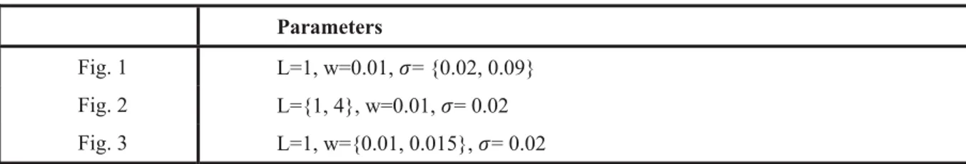
In Fig. 1, we consider production units that have a liquidation value normalized to 1 and an input cost fixed at 0.01.10 In all plots in this figure, we vary the level of volatility from a low level of ߪ ൌ ͲǤͲʹ to a medium level of ߪ ൌ ͲǤͲͻ. The resulting distributions from varying the level of volatility for each level of efficiency are plotted as two overlapping histograms: for each plot, the histograms on the left (right)correspond to higher (lower) price volatility.
Fig. 1. Exit trigger prices for separable efficiency in a Cobb-Douglas production function with simulated returns to scale for different levels of output price volatility and efficiency
Note: Parameters: ܮ ൌ ͳ, ݓ ൌ ͲǤͲͳ, ߪ ൌ ሼͲǤͲͻǡͲǤͲʹሽ, and ߠ̱ܰሺͲǤͷǡͲǤͲͲͶͻሻ. Volatility ߪ ൌ ͲǤͲͻ (left histogram) and ߪ ൌ ͲǤͲʹ (right histogram). Efficiency: ݁ିథൌ ͲǤͶͻ (upper panel), ݁ିథൌ ͲǤ (middle panel), and ݁ିథൌ ͲǤͻ (lower panel). Sample size: 10,000. One observation was excluded to avoid negative ߜԢ.
For a given efficiency level, the higher the volatility is the more reluctant firms are to exit.
This is a standard result of real options theory. It is interesting to note, however, that the impact of efficiency depends on the level of price volatility. The higher the price risk, the lower is the impact of efficiency on the optimal price trigger. Looking at the left histograms,
10 When increasing returns to scale ߠ for an input level greater than 1, an increasing marginal product calls for decreasing trigger prices if the input cost ݓ is fixed. A decreasing marginal product, however, calls for increasing trigger prices if the input level is less than 1. In these simulations, we only use levels of input cost that ensure that input levels in correspondence of the trigger prices are greater than 1.
we see a lower shift to the left when there is more efficiency. That is, in a more volatile market one can expect to find a higher heterogeneity of firms with respect to their efficiency, at least in the short run.11 The graph also shows that different firms can coexist in the market at a given exit trigger price for different efficiency levels. If only firms more efficient than a certain threshold were to be in the market for a given output price, then distributions of exit trigger prices shall not overlap for the same volatility level.
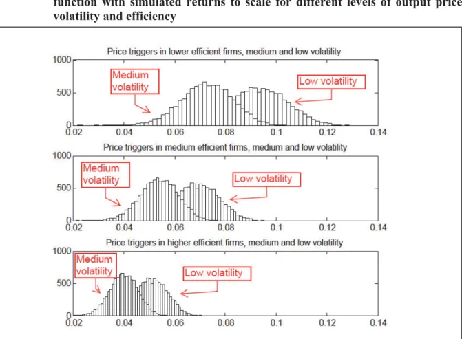
In Fig. 2, we consider what occurs when we vary the liquidation value of the production unit from 1 to 4 while keeping input cost fixed at 0.01. To isolate the effect of a varying liquidation value, we keep low the level of output price volatility, ߪ, at 0.02. At each level of efficiency, we obtain two distributions of trigger prices for each level of the liquidation value:
for each plot the histograms on the left correspond to the lower liquidation value and the histograms on the right correspond to higher liquidation value. Higher liquidation values reduce the reluctance to leave the market.
Fig. 2. Exit trigger prices for separable efficiency in a Cobb-Douglas production function with simulated returns to scale for different levels of liquidation value and efficiency levels
Note: Parameters: ܮ ൌ ሼͳǡͶሽ, ݓ ൌ ͲǤͲͳ, volatility ߪ ൌ ͲǤͲʹ, and ߠ̱ܰሺͲǤͷǡͲǤͲͲͶͻሻ. ܮ ൌ ͳ (left histogram) and ܮ ൌ Ͷ (right histogram). Efficiency: ݁ିథൌ ͲǤͶͻ (upper panel), ݁ିథൌ ͲǤ (middle panel), and ݁ିథൌ ͲǤͻ (lower panel). Sample size: 10,000.
11 This conclusion abstracts from liquidity aspects that may force firms to quit production.
In addition to shifting the distribution of exit trigger prices to the right, the higher liquidation value results in more heterogeneous reactions by firms. In particular, the reactions of less efficient firms are more heterogeneous than those by more efficient firms. The exit trigger prices for more efficient firms are more concentrated.
In Fig. 3, we consider the impact of different unit costs on exit trigger prices. We vary unit costs from 0.01 to 0.015 while the keeping liquidation value of the production units fixed at 1.
In addition, we keep the level of volatility of output price at ߪ ൌ ͲǤͲʹ.
Fig. 3. Exit trigger prices for separable efficiency in a Cobb-Douglas production function with simulated returns to scale for different levels of unit costs and efficiency levels
Note: Parameters: ܮ ൌ ͳ, ݓ ൌ ሼͲǤͲͳǡͲǤͲͳͷሽ, volatility ߪ ൌ ͲǤͲʹ, and ߠ̱ܰሺͲǤͷǡͲǤͲͲͶͻሻ. ݓ ൌ ͲǤͲͳ (left histogram) and ݓ ൌ ͲǤͲͳͷ (right histogram). Efficiency: ݁ିథൌ ͲǤͶͻ (upper panel), ݁ିథൌ ͲǤ
(middle panel), and ݁ିథൌ ͲǤͻ (lower panel). Sample size: 10,000.
For each plot, the histograms on the left (right) correspond to lower (higher) unit cost. Higher unit cost reduces the reluctance to exit the market irreversibly. Efficiency substantially influences firms that should be present in the market. In particular, it reduces the dispersion of trigger prices at which firms exit. More efficient firms tend to exit at more similar exit trigger price levels. Less efficient firms exit first, more efficient ones stay longer in the market.
To summarize the above scenarios, with increasing efficiency we find a monotonic decrease of exit trigger prices at varying degrees. This implies higher inertia for more efficient units.
3 Model extension: non-separable efficiency
In this section, we show that the relation between efficiency and exit in the separable case cannot be generalized with the same strength if efficiency is included in a non-separable manner in the production technology. A single multiplicative efficiency term restricts efficiency to act only as a shifter with respect to all production factors (Orea and Álvarez 2006). It also implies a unitary elasticity of output with respect to the efficiency term.
A natural extension is to include a non-multiplicative efficiency term. A non-multiplicative efficiency implies that efficiency cannot be separated from the inputs and output in determining the level of trigger prices. By assuming a specific functional form for non-separable efficiency and the production function, in a very simple framework we show that under decreasing returns to scale it is possible that less efficient firms are more reluctant to exit the market than more efficient ones.
3.1 Non-separable efficiency and Cobb-Douglas technology
In this subsection, we again use a Cobb-Douglas technology with one input to derive the optimal exit trigger prices. However, we now assume that the production function is directly transformed by efficiency. We rely on a Box-Cox transformation (Box and Cox 1964), but other transformations would also be possible. The observed output transformed by efficiency is:
(29) ݕ ൌሺವሺ௫ሻሻక ିଵൌ ሺ௫ഇሻకିଵ
where ߦ א ሺͲǡͳሻ is considered in this case as an efficiency parameter. The profit function then takes the form:
(30) ߨకሺǡ ݓǡ ߦሻ ൌ ିഇషభభ ݓഇషభഇ ቌቀଵకቁ ቀఏଵቁ
ഇ
ഇషభെ ቀఏଵቁ
భ
ഇషభቍ െక
where ߨకǣ Թାଷ ՜ Թା.
Second order conditions for a maximum impose that for a well-defined solution, ߦߠ ൏ ͳ.
Different combinations of returns to scale and efficiency can satisfy ߦߠ ൏ ͳ.12 To simplify the notation, we rewrite (30) as:
(31) ߨకሺǡ ݓǡ ߦሻ ൌ ܭఎെ ܦ
where ߟ ൌ െఏకିଵଵ , ܭ ൌ௪భషആఎିଵఏആ, and ܦ ൌఎିଵఎఏ 13. With this profit function, the value of the active firm should satisfy the following second order differential equation, which is analogous to (12):
12 In particular, either ߠ ൏ ͳȀߦ or ߦ ൏ ͳȀߠ.
13 The second term െܦ is mainly present because of the normalization present in the Box-Cox transformation used to provide continuity at 0. Without this, the first term most important for our results is still present.
(32) ܸԢሺሻߙ ଵଶܸԢԢሺሻߪଶଶെ ߩܸሺሻ ܭఎെ ܦ ൌ Ͳ.
Undertaking the same steps as in the previous section, we attain the following expression for the optimal exit trigger price:
(33) ఎᇱכആ ൌ ܮఉఉమ
మିఎሺଵାఈିఘሻఎᇱ כఉఉమିଵ
మିఎ
where ߟԢ ൌ ߩ െ ߙߟ െ ͳȀʹߪଶߟሺߟ െ ͳሻ is a risk adjusted discount rate. The left-hand side of equation (33) is the usual value of the net worth of the project appropriately discounted. The first term of the right-hand side is the fraction of the exit value ܮ that can be recovered upon exit from the market. This is very similar to the separable case apart from the influence of efficiency term ߦ on ߟ.
In additional, there is another term14 ሺଵାఈିఘሻఎᇱ כ, which rearranged is ሺଵାఈିఘሻఎᇱሺఎିଵሻכఎఏ and finally
ሺଵାఈିఘሻכ
కఎᇱ . This shows how efficiency and the price level interact directly. If ߦߠ ൏ ͳ then ߟ is greater than 1 and ఉఉమିଵ
మିఎ is lower than unity. Substituting back into ܭ and ܦ and rearranging terms, we obtain:
(34) ఎᇱଵ ቀכആ௪ఎିଵభషആఏആെሺଵାఈିఘሻఎିଵ כఎఏఉఉమିଵ
మିఎቁ െ ܮఉఉమ
మିఎൌ Ͳ.
Applying the chain rule allows us to see how efficiency affects (34). The derivative of ߟ with respect to ߦ is positive ሺଵିకఏሻఏ మ. Accordingly, the sign of the derivative of equation (34) with respect to ߦ15 will be the same as the sign of the derivative of (34) with respect to ߟ, given that ߟ ͳ. The latter derivative is:
(35) ఎଵᇲቆכആ௪భషആఏആ
ఎିଵ ቀכ ݓ ߠ െ ଵ
ఎିଵቁ െሺଵାఈିఘሻכሺఉమିଵሻ
ሺఉమିఎሻሺఎିଵሻ ቀିఏ
ఎିଵ ఏఎ
ఉమିఎቁቇ
ቀାቀିభమቁమቁ
ሺఎᇲሻమ ൬כߟݓߟെͳͳെߟߠߟെሺͳߙെߩߟെͳሻכߟߠߚߚʹെͳ
ʹെߟ൰ െ ܮ ఉమ
ሺఉమିఎሻమൌ Ͳ.
The signs in the first term of the derivative are positive except for כ ݓ ߠ െఎିଵଵ . The first part of the second term ቀାቀି
భ మቁమቁ
ሺఎᇲሻమ is positive. The sign depends on the second part ቀכആ௪ఎିଵభషആఏആെሺଵାఈିఘሻఎିଵ כఎఏఉఉమିଵ
మିఎቁ which can be recognized as a modified net worth of the project which by (33) shall be positive. In general, the whole derivative can be negative. In particular, for low values of the returns to scale parameter ߠ, lower efficiency can be linked to higher reluctance to exit. Under decreasing returns, very low efficient firms can be more reluctant to exit than more efficient ones. On the other hand, for higher values of ߠ, reluctance increases with efficiency.
14 Again, it is to be stressed that if we were to adopt other forms of non-separable efficiency terms, this result may not persist exist.
15 We note here that the sign of the derivative with respect to ߠ is also the same.
3.2 Simulations
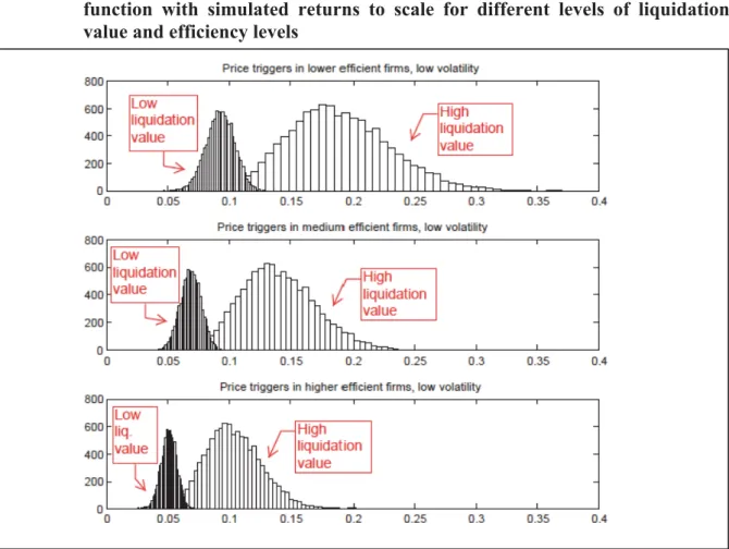
To illustrate the difference with the separable case in the previous section, we propose simula- tions that show the relationship between uncertainty, trigger prices, and a non-separable efficiency term. We illustrate the result by means of numerical simulations using similar parameter settings as in the separable case. Fig. 4 depicts the impact of efficiency under different levels of price risk (parameters: L=1, w=0.01, ߠ= 0.5, ߪ= {0.02, 0.2}). Here, we find a non-monotonic relationship for very low values of efficiency. This happens when very low levels of efficiency interact with low levels of returns to scale, which makes the degree of homogeneity of the function very low.
Fig. 4. Exit trigger prices for non-separable efficiency in a Cobb-Douglas production function with different levels of efficiency and levels of output price volatility for a medium returns to scale function
Note: Parameters: ݓ ൌ ͲǤͲͳ, ߠ ൌ ͲǤͷ, and volatility level of output prices vary from ߪ ൌ ͲǤͲʹ to ߪ ൌ ͲǤʹ.
In the following, we simulate a population of firms where the returns to scale parameter is simulated as in the separable case. To ease comparisons, for different levels of efficiency we have, as in the separable case, in each figure: in the upper plot ߦ ൌ ͲǤͷ, in the middle plot ߦ ൌ ͲǤ, and in the lower plot ߦ ൌ ͲǤͻ. An overview of the simulations parameters are provided in Table 2.
Table 2. Simulation parameters for the non-separable efficiency Cobb-Douglas case Parameters
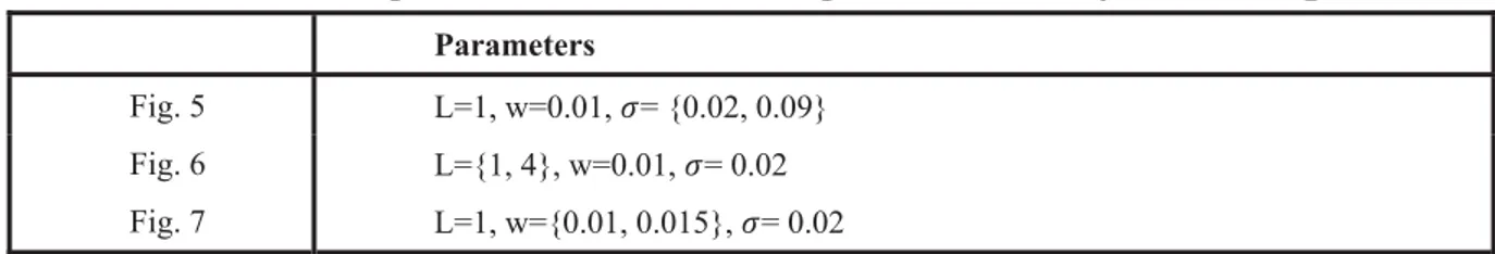
Fig. 5 L=1, w=0.01, ߪ= {0.02, 0.09}
Fig. 6 L={1, 4}, w=0.01, ߪ= 0.02 Fig. 7 L=1, w={0.01, 0.015}, ߪ= 0.02
Fig. 5 shows two series of overlapping histograms: in each plot, the histograms on the left corre- spond to higher volatility of prices (ߪ ൌ ͲǤͲͻ) and the histograms on the right correspond to lower volatility of prices (ߪ ൌ ͲǤͲʹ). Overall, the figures show a slight decrease of exit trigger prices when volatility increases for given level of efficiency. In this non-separable case, even more markedly, efficiency does not seem to discriminate between firms that should be in or out of the market.
Fig. 5. Exit trigger prices for non-separable efficiency in a Cobb-Douglas production function with simulated returns to scale for different levels of volatility of output price and efficiency levels
Note: Parameters: ܮ ൌ ͳ, ݓ ൌ ͲǤͲͳ, ߪ ൌ ሼͲǤͲͻǡͲǤͲʹሽ, and ߠ̱ܰሺͲǤͷǡͲǤͲͲͶͻሻ. Volatility ߪ ൌ ͲǤͲͻ (left histo- gram) and ߪ ൌ ͲǤͲʹ (right histogram). Efficiency: ߦ ൌ ͲǤͷ (upper panel), ߦ ൌ ͲǤ (middle panel), and ߦ ൌ ͲǤͻ (lower panel). Sample size: 10,000. Greater shifts toward left appear for a higher change in value of price risk, signaling higher reluctance to exit in the presence of higher price risk.
In Fig. 6, we consider varying the liquidation value, as in the separable case, between 1 and 4.
For each level of efficiency, for each plot the histograms on the left (right) correspond to a lower (higher) liquidation value. A higher liquidation value reduces reluctance to irreversibly exit the market. As in the separable case, with increases in liquidation values, exit trigger prices are more diversified.
Fig. 6. Exit trigger prices for non-separable efficiency in a Cobb-Douglas production function with simulated returns to scale for different levels of liquidation value and efficiency levels
Note: Parameters: ܮ ൌ ሼͳǡͶሽ, ݓ ൌ ͲǤͲͳ, ߪ ൌ ͲǤͲʹ, and ߠ̱ܰሺͲǤͷǡͲǤͲͲͶͻሻ. Liquidation value ܮ ൌ ͳ (left histogram) and ܮ ൌ Ͷ (right histogram). Efficiency: ߦ ൌ ͲǤͷ (upper panel), ߦ ൌ ͲǤ (middle panel), and ߦ ൌ ͲǤͻ (lower panel). Sample size: 10,000.
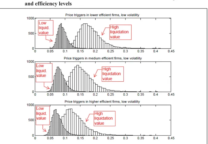
In Fig. 7, we consider the effect of varying unit costs from 0.01 to 0.015 on exit trigger prices.
For each plot, the histograms on the left (right) correspond to lower (higher) unit cost. Higher unit cost reduces reluctance to irreversibly exit the market. While we notice a clear effect on trigger prices due to higher unit costs among firms with similar efficiency levels, for the same level of costs we only notice a slight shift towards lower trigger prices when increasing efficiency. The efficiency effect seems less important when considered in a non-separable framework.
Fig. 7. Exit trigger prices for non-separable efficiency in a Cobb-Douglas production function with simulated returns to scale for different levels of unit costs and efficiency levels
Note: Parameters: ܮ ൌ ͳ, ݓ ൌ ሼͲǤͲͳǡͲǤͲͳͷሽ, and ߪ ൌ ͲǤͲʹ, ߠ̱ܰሺͲǤͷǡͲǤͲͲͶͻሻ. Input price ݓ ൌ ͲǤͲͳ (left histo- gram) and ݓ ൌ ͲǤͲͳͷ (right histogram). Efficiency: ߦ ൌ ͲǤͷ (upper panel), ߦ ൌ ͲǤ (middle panel), and ߦ ൌ ͲǤͻ (lower panel). Sample size: 10,000.
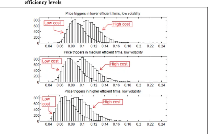
In Fig. 8, we illustrate more specifically the interaction of the level of volatility with the effect of increasing liquidation value. In particular, we note that reduction in reluctance (i.e., an increase in exit trigger prices) due to changes in liquidation value is much more pronounced for lower volatility levels than for higher ones. Higher volatility reduces the importance of the change in liquidation value.
Fig. 8. Exit trigger prices for non-separable efficiency in a Cobb-Douglas production function for high and low liquidation (exit) values, across different efficiency levels and levels of output price volatility
Note: Parameters: ݓ ൌ ͲǤͲͳ, ߠ ൌ ͲǤͷ, and liquidation value varies from ܮ ൌ ͳ to ܮ ൌ Ͷ.
Similarly, in Fig. 9 we show that the increase in exit trigger prices due to an equal increase in unit costs is proportionally lower for higher volatility levels.
Fig.9. Exit trigger prices for non-separable efficiency in a Cobb-Douglas production function for high and low unitary costs, across different efficiency levels and for levels of output price volatility
Note: Parameters: ܮ ൌ ͳ, ߠ ൌ ͲǤͷ, and input cost varies from ݓ ൌ ͲǤͲͳ to ݓ ൌ ͲǤͲͳͷ.
4 Conclusions
In this paper, we develop a model to include production efficiency in the evaluation of the exit behavior of firms when subject to a stochastic output price that follows a Geometric Brownian motion process. We do so by directly modeling the technological structure of a production firm and implicitly deriving a dual profit function through a Legendre transformation without assuming a functional form.
To exemplify this methodology, without assuming a specific functional form of the production function, a general class of results for homogeneous production functions is derived with an efficiency term separable from the rest of the production factors. More efficient firms are more reluctant to exit the market, believing in their potential to be profitable again if prices increase. Firms with a higher degree of homogeneity in inputs are generally more reluctant to irreversibly exit the market, even though this result depends on the chosen class of production functions.
These results are supported by analytical results derived for the exemplifying case of a Cobb- Douglas technology under separability of efficiency. Higher efficiency increases reluctance to exit from the market. Differently efficient production units with different returns to scale can coexist at a level of output price under the conditions developed in this study. Depending on the level of efficiency, volatility differently affects exit trigger prices.
We develop a set of numerical simulations for the specific Cobb-Douglas case to support the theoretical findings about the behavior of exit trigger prices under different efficiency levels and returns to scale. As expected, in the separable case lower efficiency increases the exit trigger prices, which raises the incentive to exit the market.
We then derive the case when the efficiency term is non-separable in a Cobb-Douglas tech- nology. Higher efficiency does not always increase reluctance to exit when very low returns to scale are present. In the numerical simulations for the non-separable case, because efficiency interacts directly with the returns to scale parameter, it has a less strong and not necessarily monotonic relationship with exit trigger prices. It seems that efficiency has a lower effect on exit trigger prices under non-separability because efficiency and returns to scale are, in a sense, substitutable in our model.
Finally, some classical results of theory of investment under uncertainty are common to all of our numerical simulations. In particular, while volatility increases reluctance to exit the market, higher unitary costs and higher liquidation values decrease the reluctance to irreversibly exit the market.
It is important to stress that our framework proposes a general methodology. Derived results are just an example of the possible assumptions on the primal technology that could result in different dual profit functions. Nonetheless, our example is general enough to show how efficiency can be included in a structural manner into the technology to derive firm exit behavior without assuming a specific production functional form.
The question of whether efficiency works as a shifter on the exit trigger or whether efficiency is non-monotonically related to the exit trigger and, if so, how it interrelates with price uncertainty needs to be answered using firm data. For example, one could use a two-stage procedure. In a first stage, the firm specific efficiency could be measured using standard approaches like a stochastic frontier analysis or data envelopment analysis. In a second stage, the predicted technical efficiency could then enter a binary choice model (stay or exit) or a hazard rate model as explanatory variable. Alternatively, firm specific efficiency and the likelihood of staying or exiting the market could be estimated jointly. Such econometric models not only allow for testing interaction effects between efficiency and uncertainty, but also allow for testing non-monotonic relations between efficiency and exit probability.
References
Box, G. E. P. and D. R. Cox (1964). An analysis of transformations. J. Roy. Stat. Soc.-B 26 (2), 211–
252.
Demsetz, H. (1973). Industry structure, market rivalry, and public policy. J. Law Econ. 16 (1), 1–9.
Dixit, A. K. (1989, June). Entry and exit decisions under uncertainty. J. Polit. Econ. 97 (3), 620–638.
Dixit, A. K. and R. S. Pindyck (1994). Investment under uncertainty. Princeton University Press.
Emvalomatis, G., S. E. Stefanou, and A. O. Lansink (2011). A reduced-form model for dynamic efficiency measurement: Application to dairy farms in Germany and the Netherlands. Am. J.
Ag. Econ. 93 (1), 161–174.
Fuss, M. and D. McFadden (1978). Production Economics: a dual approach to theory and applications.
Volume I: The theory of production. Eds. Amsterdam: North-Holland.
Goddard, E., A. Weersink, K. Chen, and C. G. Turvey (1993). Economics of structural change in agriculture. Can. J. Ag. Econ. 41 (4), 475–489.
Hüttel, S., R. Narayana, and M. Odening (2011). Measuring dynamic efficiency under uncertainty.
SiAg Working Paper 10.
Jorgenson, D. W. and L. J. Lau (1974). Duality and differentiability in production. J. Econ. Theory 9 (1), 23–42.
Kumbhakar, S. C. (2001). Estimation of profit functions when profit is not maximum. Am. J. Ag.
Econ. 83 (1), 1-19.
Kumbhakar, S. C. , E. Tsionas, and T. Sipiläinen (2009, June). Joint estimation of technology choice and technical efficiency: an application to organic and conventional dairy farming. J. Prod.
Anal. 31 (3), 151–161.
Lambarraa, F., S. E. Stefanou, and J. M. Gil (2009). The analysis of irreversibility, uncertainty and dynamic technical inefficiency on the investment decision in Spanish olive sector. 2009 Conference, August 16-22, 2009, Beijing, China 51397, International Association of Agricultural Economists, http://purl.umn.edu/51397. Accessed on 26th of July 2013.
Musshoff, O., M. Odening, C. Schade, S. C. Maart-Noelck, and S. Sandri (2012). Inertia in disinvestment decisions: experimental evidence. Eur. Rev. Agric. Econ., 40 (3), 463-485.
O’Brien, J. and T. Folta (2009). Sunk costs, uncertainty and market exit: A real options perspective.
Ind. Corp. Change 18 (5), 807–833.