urban areas for speed and travel time prediction
2
Allister Loder∗
3
IVT, ETH Zurich
4
CH-8093, Switzerland
5
Tel: +41 44 633 62 58
6
Email:aloder@ethz.ch
7
Thomas Otte
8
IMA, RWTH Aachen University
9
DE-52062, Germany
10
Tel: +49 241 809 11 64
11
Email:thomas.otte@ima.rwth-aachen.de
12
* Corresponding author
13
Paper submitted for presentation at the 100thAnnual Meeting Transportation Research Board,
14
Washington D.C., January 2021
15
Word count: 4970 words + 2 table(s)×250 + 500 (references) + 250 (abstract) = 6220 words
16
August 1, 2020
17
The prediction of journey speeds is important for decision making - not only for travelers, but
2
also for businesses such as urban freight companies. Journey speed is total travel distance divided
3
by total travel time, including all delays and additional stopping times. So far, methodologies to
4
model these interactions between cars and urban freight vehicles at an aggregated level have not
5
yet received much attention, although the demand for urban freight is growing. However, these
6
methodologies are required to identify solutions for optimal management and regulation of urban
7
freight.
8
This paper proposes a novel approach to model the interactions between cars and urban
9
freight vehicles for journey speed prediction in urban areas based on the multi-modal macroscopic
10
fundamental diagram (MFD). To ensure transferability to many applications, we formulate the
11
model in a generic way. We apply the proposed model to an synthetic network with parameters
12
oriented towards European cities to illustrate the model’s applicability and discuss trade-offs in
13
regulation of urban freight. As data related to (urban) freight movements (e.g., route planning
14
and load factors) are currently often treated as private resources by involved freight companies,
15
our generic model also provides a foundation to integrate actual freight data as soon as they are
16
available for cities as a consequence from the ongoing, continuous digital transformation. Thus,
17
the new approach not only helps cities on deriving urban freight strategies to optimize the overall
18
traffic in the network, but also helps businesses to make better decisions.
19
Keywords: urban freight transport; MFD; traffic flow; municipal decision-making; logistics; goods
20
movement
21
INTRODUCTION
1
In urban areas, many vehicles of different modes and services compete for scarce road space,
2
e.g., cars, public transport buses, pedestrians, cyclists, utility vehicles and urban freight vehicles.
3
The between-vehicle interactions among all of these vehicles create negative externalities – among
4
them additional congestion. So far, the plethora of multi-modal interactions and their congestion
5
effects in urban transportation networks have only received little attention. However, the gap is
6
beginning to close, especially the case of interactions between buses and cars (1,2) and the case of
7
ride sharing vehicles and cars (3). Contrary, among the less considered interaction cases is the case
8
between cars and urban freight vehicles (UFV) in urban areas, although the latter have a substantial
9
contribution to the urban traffic that is even expected to increase further in the following years (4).
10
In recent years, the externalities of urban freight transport (UFT) on urban areas (e.g., congestion,
11
emission of noise and pollutants) have been analyzed by, e.g., (5,6,7). In addition to the mentioned
12
works, (8) and (9) take a closer look at potential approaches to minimize the negative effects of
13
UFT and the related UFV movement inside urban areas (e.g., by shifting deliveries to off-hours).
14
In urban transportation networks with UFVs operating alongside cars, the vehicles’ journey
15
speed is an important input for business and policy decisions to optimize profits or social costs.
16
The journey speed is the total traveled distance over the total travel time and includes all delays
17
from stopping and moving. The more accurate and reliable this input becomes, the better decisions
18
can be made. In urban traffic, cars and UFVs interact physically due to their different behavior
19
and vehicle dimensions. For example, UFVs stop more frequently and for other purposes (e.g., for
20
delivering shipments) than cars and their acceleration is slower. These interactions make a reliable
21
speed prediction more complex and difficult. As physical vehicle interaction always leads to a
22
decrease in all vehicles’ journey speeds, too optimistic journey speed predictions could be costly
23
for businesses and could lead to inefficient control and regulation measures as well as long-term
24
infrastructure investment decisions for the urban transportation network. So far, however, methods
25
to capture these interaction delays in the journey speed prediction for car and UFV traffic in urban
26
areas at the network level are not existing.
27
In this paper, we use recent advances in macroscopic modeling of vehicles’ journey speed in
28
urban transportation networks with the macroscopic fundamental diagram (MFD) (10,11,12,13)
29
to address this gap. Based on the MFD, we propose a model that makes interaction speeds of
30
cars and UFVs better predictable, likely to improve business and policy decisions. The underlying
31
modeling idea is that bi-modal urban network traffic consisting of cars and UFVs is similar to
32
bi-modal urban traffic consisting of buses and cars, for which a variety of flexible and promising
33
approaches already exist (1, 2, 14, 15), but with the difference that many UFV network design
34
parameters are random variables rather than fixed parameters, e.g., stop distance, stop duration,
35
vehicle headway.
36
The transferability of bus network modeling approaches to urban freight follows from three
37
main reasons: first, the obstruction on the road is happening mostly on the curb-side lane, e.g.,
38
buses and UFVs double park when no separate infrastructure is available. Second, UFV operations
39
share various similarities with buses such as driving from stop to stop to perform their service at
40
each stop, while UFVs are expected to stop longer than buses. Third, the involved operators are
41
faced with similar design questions (e.g., route planning, headway). Thus, using existing methods
42
for bi-modal traffic with buses for UFV operations could achieve more reliable and accurate speed
43
predictions.
44
To predict journey speeds accurately from an aggregated network perspective, one key
45
aspect is to understandwhena bottleneck is activated and congestion starts to emerge in the urban
1
transportation network. For buses operating on a regular schedule, the bottleneck activation is quite
2
deterministic, whereas UFVs do not operate on a regular schedule, but have their routes, delivery
3
stop locations and their headway (the number of required vehicles) planned based on shipment
4
demand (origin, destination, time). With bottleneck activation by UFVs being a random process, its
5
microscopic prediction is difficult, while its macroscopic prediction relies on the expected values of
6
these random variables describing UFV operations. Another aspect that supports the macroscopic
7
approach is the limited availability of microscopic freight transport data (e.g., actual temporal and
8
spatial movement of UFVs) as addressed by, for example, (6, 16). For example, (16) address
9
the potential benefits of an increased and centralized (i.e., consolidated at a central point that is
10
administered by municipal decision-makers) data availability for the quality of municipal decision-
11
making processes as well as their positive effect on the urban transportation network. Various
12
research efforts exist to enhance data availability and accessibility (cf. reviews (6,17,18)), where
13
especially for filling the gap of microscopic data availability respectively central data accessibility
14
between different actors, various methods can be applied reaching from simulation (cf. (19) to
15
empirical data collection (cf. (20).
16
To illustrate the model’s applicability and discuss trade-offs in regulation of urban freight,
17
we apply the proposed journey speed prediction model to an synthetic network with parameters
18
oriented towards European cities. The parameters’ values are taken from freight activities in Ham-
19
burg, Cologne and Nuremberg, where BIEK (i.e. German Parcel and Express Logistics Associa-
20
tion, a domain-related association) publishes aggregated freight data on a regular basis.
21
In the following, we summarize first the fundamental concepts of each associated domain,
22
namely urban freight transport and macroscopic traffic modeling to make all readers familiar with
23
these concepts. Then we show how the interaction delays between cars and UFVs can be captured
24
at an aggregated network perspective for journey speed prediction. Thereafter, we show for ap-
25
plicability of the speed prediction model for policy scenario analyses. We end this paper with a
26
discussion and outlook for future research.
27
LITERATURE REVIEW
28
Predicting journey speeds in urban areas of mixed traffic with UFVs and cars requires knowledge
29
from at least three domains. First, how urban freight transport is organized and how it interacts
30
with other urban transportation systems. Second, how UFVs routes are obtained from supply of
31
vehicles and demand of shipments. Third, how speed can be predicted given the presence and flow
32
of vehicles. In the following, we present the fundamental concepts for each of the three domains.
33
Urban Freight Transport
34
The domain of urban freight transport (UFT) has been on the agenda of researchers for more than
35
two decades until now. In recent years, various overarching works have been presented by, for
36
example, (7), (6) and (21) with regard to UFT as well as directly related terms like for instance:
37
city logistics,urban logistics,urban goods movementandurban freight distribution.
38
One sub-topic inside the UFT domain is freight demand management (FDM). (5) define
39
FDM as ’the area of transportation policy that seeks to influence the demand generator - to achieve
40
urban freight systems that increase economic productivity and efficiency; and enhance sustainabil-
41
ity, quality of life, and environmental justice’ and understand it as the freight-related equivalent to
42
passenger demand management. Exemplary measures in FDM are initiatives fortemporal delivery
43
shifts(e.g., to off-hour or to off-peak) or forreceiver-led consolidation(e.g., by coordinating with
1
similar demands in the proximity). Aiming at sustainable urban freight systems, (5) showed that
2
FDM can have significant contribution to reducing both the freight traffic as well as the overall
3
traffic and thus the congestion inside the urban transportation network.
4
In their recent work, (22) suggested further approaches for the sustainable and efficient
5
integration of UFT into the urban transport network. Among others, they assign a central role to
6
the coordination of deliveries and suggest further investigations with this focus. The suggestion has
7
been picked up by (16) and (23) as a starting point to identify additional approaches to increasing
8
coordination in urban delivery processes. To contribute to the further development of cities in
9
the direction ofsmart cities, they study the potential benefits of an increased and centralized (i.e.,
10
collected from various data sources and consolidated in a central data infrastructure) availability
11
of both macroscopic and microscopic freight data for municipal decision-making processes. From
12
their perspective, the data availability is expected to increase in the course of the following years
13
as a consequence of the continuous digital transformation of existing business processes. Based
14
on that, enabling cities to access and process available freight data would be crucial in order for
15
cities to meet their responsibility to, on the one hand, maximize the productivity and efficiency of
16
the urban transportation network, while, on the other hand, minimizing the negative side effects of
17
the associated traffic volume - in particular: congestion and emissions.
18
Vehicle Routing Problems
19
The operations of UFVs are faced with a variety of mathematical optimization tasks, e.g., rout-
20
ing, capacity planning, scheduling. Typically, these tasks represent combinatorial optimization
21
problems that aim at finding an optimal solution inside a pre-defined search space.
22
One prominent problem is theVehicle Routing Problem (VRP)that is used to planoptimal
23
routes for delivering shipments using an existing vehicle fleet. The objective is to assign a set of
24
vehicles to a set of customers to satisfy their demands while minimizing the total traveled distance.
25
The vehicles start their tour at a central depot and return to the same depot after finalizing the
26
planned tour.
27
Originating from that basic VRP principle, different types of VRP exist and can be classi-
28
fied, for example, based on involved constraints, e.g., acess time windows, environmental cost. An
29
overview on VRP in the UFT domain can be found, for example, in (24). VRPs also occur beyond
30
the UFT domain - structured overviews on existing VRPs have been presented by, for example,
31
(25) and (26).
32
Macroscopic Fundamental Diagram
33
Predicting journey speeds in urban road networks on an aggregate level has been of interest since
34
more than fifty years (27,28) with its most recent development being the macroscopic fundamental
35
diagram (MFD) (11). The general idea is to predict not only the average journey speed, but also its
36
distribution in the network as a function a variables that cover the demand and physical properties
37
of the network. Predicting speeds on an aggregate level with the MFD is much faster than using a
38
traffic simulator, but slightly less accurate (29).
39
The MFD, originally for car transportation only, describes the relationship between the
40
number of vehicles circulating in the network N and their collective production of vehicle kilo-
41
metersΠ and journey speedv of vehicles that includes all driving and standing time throughout
42
the journey. Figure 1 shows the typical MFD shape: while production of vehicle kilometers first
43
a
𝑁
b
𝑁
𝑣Π
FIGURE 1 : Typical MFD shape: a travel production-accumulation relationship; b speed- accumulation relationship.
increases with the number of vehicles until congestion starts and production decreases with the
1
number of vehicles as Figure 1a, the average journey speed declines with the number of vehicles
2
in the network due to congestion as seen in Figure 1b.
3
The shape of the MFD is a characteristic fingerprint of each network and can either be
4
obtained analytically or from measurements (simulation, stationary detectors or floating car data)
5
(30). Multi-modal interactions between different transport modes are captured in multi-modal
6
MFDs that quantify the joint travel production and network average journey speed of all modes
7
as a function of each modes’ vehicle accumulation. Multi-modal MFDs can also be estimated
8
analytically (15, 31, 32) or from measurements (1, 2), where the analytical methods reportedly
9
face difficulties in capturing the complexity of multi-modal traffic in multi-modal MFDs, leaving
10
the measurement method as the robust alternative.
11
MODELING CAR AND UFV INTERACTIONS
12
The proposed speed model links the number of cars NC and number of UFVsNU FV in an urban
13
road network to their respective average journey speedvCandvU FV. These journey speeds include
14
the interaction effects of the two vehicle types as well as any stopping and moving time inside
15
the urban transportation network. Thus, we have to focus on stopping and moving time to fully
16
understand journey speeds (33). In the following paragraph, we present the assumptions for the
17
speed prediction model to model car-UFV interactions.
18
First, in Figure 2awe illustrate an abstract sequence of events involved in a typical ship-
19
ment delivery process, an UFV stopping process that creates a temporal bottleneck for other ve-
20
hicles in the network that are consequently experiencing longer stopping times. It can be derived
21
from Figure 2a that many factors influence the stopping time of UFVs, e.g., distance between
22
parking position and target destination in step 1 or visibility and accessibility of building entrance
23
in step 4. Second, the dimensions (e.g., weight) of UFVs are larger compared to cars, impacting
24
their acceleration. This leads to the behavior shown in Figure 2b where the two vehicle types’
25
moving speeds (not journey speeds) converge in congestion, while in free flow UFV speeds are
26
slightly lower than car speeds due to reduced acceleration. Third, the urban freight network design
27
b c
Route 1
Depot
Route 2
Vehicle Route t x y
𝑣! 𝑣"#$
=𝑣! 𝑣"#$,&'(
𝑣"#$
a
1. Park UFV 2. Unload
Shipment(s) 3. Lock UFV 4. Search Building
Entrance …
… 5. Ring and
Wait
6. Climb Stairs or Take
Elevator
7. Deliver
Shipment 8. Return to UFV
FIGURE 2: aTypical shipment delivery process following (34),bspeed relationship of cars and UFV due to differences in acceleration,cidealized vehicle routing graph with its key variables.
variables and many delivery process variables from Figure 2a are stochastic processes where the
1
bottleneck is not activated on a regular basis. Fourth, the UFV operator determines the routes, the
2
sequence of delivery stops and the amount of shipments for each UFV before all vehicles leave the
3
depot as seen in the vehicle routing graph in Figure 2c. In other words, the number of stops, the
4
stop locations and the (planned) routes are, determined either manually or automated using, e.g.,
5
VRP solvers (commercially available software), known for all UFVs in the network once they are
6
circulating. They are not changed during a tour, e.g., due to congestion. Once a UFV delivered all
7
shipments, it returns to the depot.
8
The input of the model, i.e., NC and NU FV, are linked to the output of the model, i.e., vC
9
andvU FV, using the multi-modal MFD as shown in Eqn. 1. The interactions are captured in the
10
multi-modal MFD using the two-fluid theory of town traffic (33) for car traffic, extended to the
11
multi-modal MFD (35).
1
vC, vU FV
=MFD
NC, NU FV
(1) The average journey speed expressed in the MFD includes the moving and stopping times
2
of all vehicles inside the network. Therefore, multi-modal interaction delays can be separated into
3
the average additional time for moving pm and stopping ps per unit distance that is nothing else
4
than the impact on pace, the inverse of speed (35). Then, the total pace of vehicles pcorresponds
5
to the pace without interactions p0and the two delayspmand ps as shown in Eqn. 2.
6
p=p0+pm+ps (2)
In this particular interaction case of cars and UFVs, we consider that the differences in
7
vehicle dimensions create additional moving delays for cars pm and that the delivery stopping
8
process creates additional stopping delayspsfor cars. In the following two subsections, we explain
9
each of the mentioned, additional delays in detail.
10
Moving delays
11
For the moving delays, let us first define thatϑ indicates the moving speed of vehicles that does
12
not include any stopping times. Thus, this speed differs from the average network speedvfrom the
13
MFD. The moving delays pmresult from the different vehicle dimensions, leading to the behavior
14
observed in Figure 2b. Recall that the moving speeds of both vehicle types differ in the free flow,
15
but converge in congestion. The additional moving delays for each vehicle can the be obtained
16
using Eqn. 3 as the difference in moving speeds that include vehicle interactions with other vehicle
17
typesϑinteractionand are without vehicle interactions with other vehicle typesϑno interaction.
18
pm= 1 ϑinteraction
− 1
ϑno interaction
(3) Stopping delays
19
We derive from Figure 2a that the total delivery time per stop τ results from two main factors,
20
namely urban topographyT (e.g., building accessibility, number of floors) and the delivery process
21
D(e.g., total amount of shipments per stop, amount of shipments per delivery, average dimension
22
of a single shipment, distribution of shipments at a stop location, availability of parking areas).
23
We consider that the average delivery stopping time in a network isτ in units seconds per stop is
24
network-specific and captures, e.g., parking behavior and policy, and must be calibrated from data.
25
We propose to model the delay per stopτ inspired by a Cobb-Douglas production function
26
with inputsT andDas introduced in Eqn. 4. The inputsT andDare, like in economics, aggregated
27
variables that can be, but are not limited to, the examples from the previous paragraph. We adopt
28
such a macroscopic and aggregated perspective to ensure that this framework applies to as many
29
different delivery processes as possible. Consequently, for each specific application, the inputsT
30
andDhave to be customized.
31
τ =τ·TθT·DθD (4)
This Cobb-Douglas formulation not only naturally ensures that τ >0, but also uses pa-
32
rametersθT and θD as output elasticities. They allow to adjust or determine whether delays are
33
produced with increasing, decreasing or constant returns to scale. The inputs can also be under-
1
stood as intermediate goods and are thus themselves outputs of another production function. We
2
define the specific inputs forT andDin the next section, where we show policy analyses with this
3
model. With inputs specified for an UFV application, all the parameters must be calibrated from
4
data.
5
Importantly,τis for a single stop, but Eqn. 2 requires the additional stopping delay per unit
6
distance. Therefore, we scale each stop’s delayτ by the average distance between UFV stopsdas
7
given in Eqn. 5 that results from the vehicle routing graph.
8
ps= τ
d (5)
Inhomogeneity of delays
9
The delays expressed in Eqns. 3 and 5 assume a homogeneous presence of delays along an urban
10
corridor. In their current formulation, they are formulated such that every car would experience
11
pm and ps. In real urban road networks, not every car is experiencing these delays all the time,
12
however, every car is experiencing the average delays from interacting and not interacting with
13
UFVs along its journey. Thus, let us define thatP is a random variable for moving and stopping
14
separately. Each variable has outcomes P= p in case of interactions and P=0 in case of no
15
interactions. Then, the expectation of additional delays can be obtained as formulated in Eqn. 6.
16
E[P] =0·Pr(P=0) +p·Pr(P=p) = p·Pr(P= p) (6) There are two ways to obtain information about the probabilities Pr. First, learn them from
17
data which is possible for UFV operators because they have access to their vehicles’ trip recorders
18
and to commercially available car speed recordings. Second, if no such access to data exists, they
19
can be approximated using (analytical) formulae. As this data is currently not available, we can
20
only introduce the idea to learn the probabilities from data. Until the data becomes available, we
21
approximate, and thus simplify, the probabilities for the moving process with a uniform distribution
22
(encountering a UFV while driving corresponds to the fraction of UFVs from all vehicles) and for
23
the stopping process with a binomial distribution (encountering one, two, N-times an UFV stopping
24
per unit distance) following the ideas discussed by (35).
25
POLICY SCENARIOS: MANAGING URBAN FREIGHT
26
In this policy analyses we study four different scenarios of parcel delivery in dense urban areas
27
with the previously introduced speed model for an abstract synthetic network. The delivery process
28
is assumed to follow the sequence in Figure 2a. We focus on scenarios that emphasize different
29
features of UFV operations and that are discussed for UFV regulation (e.g., (9)): (1) all-day normal
30
UFV operations, (2) restricting UFV operations during peak times, (3) more recipients at delivery
31
stops for the same amount of shipments, (4) cooperation of UFV operators that increases routing
32
and vehicle loading efficiency. All scenarios are compared for the same exogenous, dynamic
33
loading profile of cars in the network.
34
For this parcel delivery service, we define thatT (urban topology) andD(delivery process)
35
follow production functions like Eqn. 4. All inputs intoT andDare normalized by their calibra-
36
tion value. This ensures thatτ =τ (the average delivery duration) holds at the calibration point.
37
Furthermore, each input has an output elasticity ofθ that can capture whether delays are produced
38
with decreasing, constant or increasing returns to scale.
39
First, urban topographyT is expressed by the number of floors of buildingsH as defined
1
in Eqn. 7. Intuitively, for parcel delivery services, the average delivery time increases with the
2
average number of building floors in the city.
3
T = H
H θH
(7) Second, we consider thatDresults from the average amount of shipments per delivery stop
4
S, the average shipment dimensions (e.g., weight and volume)W, and the distribution of shipments
5
to recipients at a delivery stop, expressed in the Gini indexG. For G=1, one recipient receives
6
all the shipments, while forG=0, each shipment has another recipient. WhenS,W orGincrease,
7
the average delivery stopping time increases. Eqn. 8 shows the resulting production function for
8
D.
9
D= S
S θS
· W
W θW
· S+G(1−S) S+G 1−S
!θG
(8) For this policy analyses, we parameterize the functions with data from a survey on UFV
10
parcel delivery operations from German cities (34,36). We summarize the resulting parameters of
11
UFV operations and of the defining features of the abstract synthetic network in Table 1. The urban
12
transportation network has a symmetrical grid layout with 15 blocks of 100 m length on each side.
13
Thus, the network covers an area of 2.25 km2. Dense German cities reportedly have a demand of
14
at least 1000 parcels per km2and day (34,36) that we scale to a total demand of 10000 shipments
15
in the network for the policy analyses to describe high demand seasons, e.g. Christmas. We define
16
that the resulting parameters of the vehicle routing algorithm for UFVs are those given in Table 2.
17
Last, we set the output elasticities as followsθT =0.3,θD=0.7 andθH=θS=θW =θG=1. The
18
first two elasticities, we assume thatD has a greater impact than T on delays, while for the last
19
three elasticities we assume that all contribute equally to delays with increasing returns to scale.
20
In all four scenarios, we load the road network with the same exogenous time-series of car
21
accumulation shown in Figure 3a with a direct assignment. This series exhibits common distinct
22
morning and evening peaks with a smaller lunch-time peak. We assume that the VRP results for
23
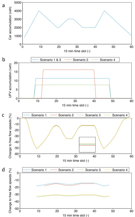
each scenario in the number of UFVs shown in Figure 3bas well as UFV operation parameters
24
given in Table 2. Note that the accumulation of UFVs is approximately two orders of magnitude
25
smaller than the accumulation of cars. We simulate the effect of UFV operations in 60 time slices of
26
15 min duration, i.e. ranging from 6:00 AM to 9:00 PM. As seen in Figure 3b, the UFV operation
27
hours in Scenarios 1, 3 and 4 range from 8:00 AM to 6:00 PM (e.g., as defined by the maximum
28
work allowance of a single driver), the limited operation hours for Scenario 2 range from 9:00 AM
29
to 4:00 PM. We follow a static accumulation-based perspective by considering the accumulation
30
of cars and UFVs fixed in each simulation interval and predict the speeds of each mode based on
31
the multi-modal MFD.
32
In Figures 3c-dwe then show the resulting speeds of cars and UFVs, respectively. In Figure
33
3cwe find the expected speed pattern resulting from the car accumulation pattern from Figure 3a
34
with speeds dropping to more than half the network average space-mean speed in the morning and
35
evening peak. In the congested time slots, we do not see an impact of the few UFVs (less than 20
36
UFVs compared to more than 4000 cars) as in congestion speeds of all modes typically converge.
37
Contrary, in the less congested time slots, we find an impact of the UFVs with Figure 3’s inlay
38
Network
Total network length 100 lane-km Average number of lanes per street 3
Blocks of 100 m length 15
UFVs
Total shipments 10 000
Number of stops per tour 100
Tour distance 60 km
Average stopping time per stop (τ) 4.5 min
Tour per vehicle and day 1
Free-flow moving speed 28 km/h
MFD capacity 0.1 veh/s
MFD jam density 0.1 veh/m
Cars
Free-flow moving speed 35 km/h
MFD capacity 0.149 veh/s
MFD jam density 0.145 veh/m
Interaction
H 1
W 1
S 2
G 1
θT 0.3
θD 0.7
θH =θS=θW =θG 1
TABLE 1 : Model parameters that are oriented towards European cities (cf. (2, 37)). As men- tioned, this delay model uses the methodology by (35) that requires more interaction parame- ters. Those not listed above are similar to those given by (35) for cars and buses, except for λcar=λU FV =0.01.
Scenario Defining feature Operation hours Shipments per stop Stops per hour
1 Normal operations 10 2 10
2 Limited operation hours 7 2 10
3 More recipients at delivery stops 10 2 10
4 Cooperation 10 3 11
TABLE 2: UFV operation parameters for each considered scenario.
0 1000 2000 3000 4000 5000
Car accumulation (veh)
0 10 20 30 40 50 60
15 min time slot (-)
-60 -50 -40 -30 -20 -10 0
Change to free flow speeds (%)
0 10 20 30 40 50 60
15 min time slot (-)
Scenario 1 Scenario 2 Scenario 3 Scenario 4
-50 -40 -30 -20 -10 0
Change to free flow speeds (%)
0 10 20 30 40 50 60
15 min time slot (-)
Scenario 1 Scenario 2 Scenario 3 Scenario 4
slot
0 5 10 15 20
UFV accumulation (veh)
0 10 20 30 40 50 60
15 min time slot (-)
Scenario 1 & 3 Scenario 2 Scenario 4
a
b
c
d
FIGURE 3: Results of the scenario analysis for UFV operations.aCar accumulation time-series for the simulation, bUFV accumulation time-series,cresulting changes in car journey speeds,d resulting changes in UFV journey speeds.
allowing to distinguish the four scenarios. The speed reduction is increasing from Scenario 4,
1
Scenario 1, Scenario 3 to Scenario 2 and results from the impact of UFV accumulation and stops.
2
The order is intuitive as Scenario 4 operations are optimized, while in Scenario 2 more stops per
3
hour are required to deliver all shipments, increasing the delays for cars.
4
In Figure 3dwe find that the network average space-mean speed of UFVs is substantially
5
below its free-flow speed resulting from the interaction with car traffic. The speeds in Scenario
6
3 and 4 are even lower due to increased number of stops and stopping times. Importantly, this
7
accumulation-based direct assignment does not consider whether shipments cannot be delivered
8
due to delays or UFVs have to circulate longer in the network, but both have a negative impact on
9
congestion and economics.
10
The results clearly emphasize the impact of bi-modal traffic of car and UFVs on car speeds
11
as well as UFV speeds. Even when the number of UFVs is small compared to the car accumulation,
12
an impact is seen which would be even amplified with more UFVs in the network. Nevertheless,
13
the results also emphasize the need for calibration and specification for the many specific UFV
14
operation systems that are in place in urban areas to capture the entire system dynamics.
15
DISCUSSION
16
In this paper, we presented a novel approach to model the interactions between cars and urban
17
freight vehicles in urban areas based on the macroscopic fundamental diagram (MFD). Information
18
on journey speeds that include interaction delays in multi-modal traffic are important not only for
19
businesses to make better decisions, but also for cities in order to derive optimal strategies, e.g.,
20
for managing urban freight deliveries. The interactions are captured in the journey speeds using
21
the two-fluid theory of town traffic (33) extended to the multi-modal MFD (35). We formulated
22
the model abstractly to ensure transferability to as many problems for different delivery processes
23
(e.g., vehicle routing or scheduling) as possible. When customizing the model for each specific
24
application, the data required for calibrating the model is available to urban freight fleet operators
25
(e.g., as an output of their fleet planning and vehicle routing problem calculations) and should
26
be shared with municipal decision-makers in order to calculate network-optimal solutions as this
27
will lead to long-term benefits (e.g., less congestion, higher journey speeds, higher delivery-trip
28
productivity, higher profitability) for each involved fleet operator with their individual intentions
29
(e.g., profit optimization) (16). Last, we showed the applicability of our proposed model to study
30
urban freight regulation and management scenarios.
31
The proposed speed model can be included in many optimization problems where the num-
32
ber of vehicles and their journey speed are key variables. These problems are found on the UFV
33
operator side, e.g., fleet management and routing, as well as on the municipal decision-maker side,
34
e.g., parking regulations or traffic control. Thus, when properly calibrated and validated, the model
35
and its resulting optimization problems allow to improve operations strategies in order to save costs
36
and improve service quality. Future research, therefore, should build this speed prediction model
37
as a module into applications relevant for fleet operators as well as municipal decision makers in
38
order to exploit the benefits of an increased prediction quality (e.g., in vehicle routing problems of
39
fleet operators or traffic volume and traffic flow predictions of municipal decision-makers).
40
The policy analyses in the previous section shows how the model applies for speed pre-
41
diction associated questions, while it also emphasizes that data is required for the calibration and
42
more importantly for deriving implications, but also for validation of the speed prediction model.
43
Such data is already available for UFV fleet carriers, but usually not for cities. However, new data
44
collection methods using technologies such as drones (37) allow to measure all interactions and
1
trajectories required for the calibration of speed prediction models like ours. In addition, macro-
2
scopic traffic data is also becoming more widely available that help to define bounding boxes speed
3
prediction models’ parameters. Only the availability of such data then allows to identify when and
4
where this simplification of reality is adding value for decision making. Thus, future research could
5
engage in finding methods to obtain the model parameters, especially the interaction probability,
6
with high accuracy for improving decision making.
7
The fact that freight data availability outside private companies is still one central issue
8
for cities as well as researchers indicates an (ongoing) gap between research and practice. As al-
9
ready highlighted by (38) more than ten years ago, exploiting long-term benefits for the overall
10
(urban) transportation network with measures such as consolidation, cooperation, or route opti-
11
mization still seems to be a comparatively idealistic goal as the freight transport market is highly
12
competitive. Thus, incentives for data exchange between private companies and cities as well as
13
researchers are needed in order to bridge the gap of data availability. In this course, it will be par-
14
ticularly important for the incentive measures to quantify and communicate the potential benefits
15
of a data exchange to the involved private actors as this might, in the next step, enable them to eval-
16
uate their risks and recognize their potential individual benefits (e.g., saving costs through better
17
speed predictions) which could subsequently leverage them to cooperate. Future research could
18
therefore focus on laying the foundation for the data exchange, especially by developing technical
19
frameworks for the data exchange (ensuring data security) as well as for the data storage (ensuring
20
data anonymization).
21
In closing, the growing demand for mobility in urban areas together with growing demand
22
for shipments increase the load on the urban infrastructure and calls for improvement management
23
as well as regulation of multi-modal traffic. This proposed model can help to make better decisions
24
for businesses and society, thus could lead to make urban traffic more sustainable.
25
AUTHOR CONTRIBUTION STATEMENT
26
The authors confirm contribution to the paper as follows: AL and TO conceived and conducted the
27
study as well as wrote the manuscript. AL developed the code.
28
References
29
[1] Geroliminis, N., N. Zheng, and K. Ampountolas, A three-dimensional macroscopic funda-
30
mental diagram for mixed bi-modal urban networks.Transportation Research Part C: Emerg-
31
ing Technologies, Vol. 42, 2014, pp. 168–181.
32
[2] Loder, A., L. Ambühl, M. Menendez, and K. W. Axhausen, Empirics of multi-modal traffic
33
networks – Using the 3D macroscopic fundamental diagram.Transportation Research Part
34
C: Emerging Technologies, Vol. 82, 2017, pp. 88–101.
35
[3] Erhardt, G. D., S. Roy, D. Cooper, B. Sana, M. Chen, and J. Castiglione, Do transportation
36
network companies decrease or increase congestion? Science Advances, Vol. 5, No. 5, 2019,
37
p. eaau2670.
38
[4] World Economic Forum,The Future of the Last-Mile Ecosystem: Transition Roadmaps for
39
Public- and Private-Sector Players, 2020.
40
[5] Holguín-Veras, J., I. Sánchez-Díaz, and M. Browne, Sustainable Urban Freight Systems and
41
Freight Demand Management.Transportation Research Procedia, Vol. 12, 2016, pp. 40–52.
42
[6] Lagorio, A., R. Pinto, and R. Golini, Research in urban logistics: a systematic literature
43
review. International Journal of Physical Distribution & Logistics Management, Vol. 46,
1
No. 10, 2016, pp. 908–931.
2
[7] Dolati Neghabadi, P., K. Evrard Samuel, and M. L. Espinouse, Systematic literature review
3
on city logistics: overview, classification and analysis.International Journal of Production
4
Research, Vol. 57, No. 3, 2018, pp. 865–887.
5
[8] Browne, M., Allen, Julian, Nemoto, Toshinori, D. Patier, and J. Visser, Reducing Social
6
and Environmental Impacts of Urban Freight Transport: A Review of Some Major Cities.
7
Procedia - Social and Behavioral Sciences, Vol. 39, 2012, pp. 19–33.
8
[9] Sánchez-Díaz, I., P. Georén, and M. Brolinson, Shifting urban freight deliveries to the off-
9
peak hours: a review of theory and practice.Transport Reviews, Vol. 37, No. 4, 2017, pp.
10
521–543.
11
[10] Daganzo, C. F., Urban gridlock: Macroscopic modeling and mitigation approaches.Trans-
12
portation Research Part B: Methodological, Vol. 41, No. 1, 2007, pp. 49–62.
13
[11] Geroliminis, N. and C. F. Daganzo, Existence of urban-scale macroscopic fundamental
14
diagrams: Some experimental findings. Transportation Research Part B: Methodological,
15
Vol. 42, 2008, pp. 759–770.
16
[12] Loder, A., L. Ambühl, M. Menendez, and K. W. Axhausen, Understanding traffic capacity of
17
urban networks.Scientific Reports, Vol. 9, No. 16283, 2019.
18
[13] Paipuri, M., Y. Xu, M. C. González, and L. Leclercq, Estimating MFDs, trip lengths and path
19
flow distributions in a multi-region setting using mobile phone data.Transportation Research
20
Part C: Emerging Technologies, Vol. 118, No. January, 2020, p. 102709.
21
[14] Daganzo, C. F., Structure of competitive transit networks. Transportation Research Part B:
22
Methodological, Vol. 44, No. 4, 2010, pp. 434–446.
23
[15] Loder, A., I. Dakic, L. Bressan, L. Ambühl, M. C. Bliemer, M. Menendez, and K. W.
24
Axhausen, Capturing network properties with a functional form for the three-dimensional
25
macroscopic fundamental diagram. Transportation Research Part B: Methodological, Vol.
26
129, 2019, pp. 1–19.
27
[16] Otte, T., A. Fenollar Solvay, and T. Meisen, The future of urban freight transport: Shifting
28
the cities role from observation to operative steering.Proceedings of 8th Transport Research
29
Arena TRA 2020, April 27-30, 2020, Helsinki, Finland, 2020.
30
[17] Patier, D. and J.-L. Routhier, How to Improve the Capture of Urban Goods Movement Data?
31
InTransport Survey Methods(P. Bonnel, M. Lee-Gosselin, J.-L. Madre, and J. Zmud, eds.),
32
Emerald Publishing Limited, Bingley, 0, 2009, pp. 251–287.
33
[18] Ambrosini, C. and J.-L. Routhier, Objectives, Methods and Results of Surveys Carried out
34
in the Field of Urban Freight Transport: An International Comparison.Transport Reviews,
35
Vol. 24, No. 1, 2004, pp. 57–77.
36
[19] Russo, F. and A. Comi, A modelling system to simulate goods movements at an urban scale.
37
Transportation, Vol. 37, No. 6, 2010, pp. 987–1009.
38
[20] Gonzalez-Calderon, C. A., I. Sánchez-Díaz, I. Sarmiento-Ordosgoitia, and J. Holguín-Veras,
39
Characterization and analysis of metropolitan freight patterns in Medellin, Colombia.Euro-
40
pean Transport Research Review : An Open Access Journal, Vol. 10, No. 2, 2018, pp. 1–11.
41
[21] Lindholm, M., Urban freight transport from a local authority perspective-A literature review.
42
European Transport, , No. 54, 2013.
43
[22] Sánchez-Díaz, I. and M. Browne, Accommodating urban freight in city planning.European
44
Transport Research Review : An Open Access Journal, Vol. 10, No. 2, 2018, pp. 1–4.
45
[23] Otte, T., A. Gannouni, and T. Meisen, The future of urban freight transport: A data-driven
1
consolidation approach to accompany cities on their path to zero redundancy in freight move-
2
ment.27th ITS World Congress, Los Angeles, USA. (accepted after peer-review, conference
3
canceled due to ongoing COVID-19 pandemic), 2020.
4
[24] Cattaruzza, D., N. Absi, D. Feillet, and J. González-Feliu, Vehicle routing problems for city
5
logistics.EURO Journal on Transportation and Logistics, Vol. 6, No. 1, 2017, pp. 51–79.
6
[25] Adewumi, A. O. and O. J. Adeleke, A survey of recent advances in vehicle routing problems.
7
International Journal of System Assurance Engineering and Management, Vol. 9, No. 1,
8
2018, pp. 155–172.
9
[26] Pillac, V., M. Gendreau, C. Guéret, and A. L. Medaglia, A review of dynamic vehicle routing
10
problems.European Journal of Operational Research, Vol. 225, No. 1, 2013, pp. 1–11.
11
[27] Smeed, R. J., Traffic studies and urban congestion. Journal of Transport Economics and
12
Policy, Vol. 2, 1968, pp. 33–70.
13
[28] Mahmassani, H., J. C. Williams, and R. Herman, Performance of urban traffic networks. In
14
10th International Symposium on Transportation and Traffic Theory(N. Gartner and N. H. M.
15
Wilson, eds.), Elsevier Science Publishing, 1987.
16
[29] Dandl, F., G. Tilg, M. Rostami-Shahrbabaki, and K. Bogenberger, Network Fundamental
17
Diagram Based Routing of Vehicle Fleets in Dynamic Traffic Simulations. IEEE Access,
18
2020.
19
[30] Leclercq, L., N. Chiabaut, and B. Trinquier, Macroscopic fundamental diagrams: A cross-
20
comparison of estimation methods.Transportation Research Part B: Methodological, Vol. 62,
21
2014, pp. 1–12.
22
[31] Dakic, I., L. Ambühl, O. Schümperlin, and M. Menendez, On the modeling of passenger
23
mobility for stochastic bi-modal urban corridors.Transportation Research Part C: Emerging
24
Technologies, Vol. 113, 2020, pp. 146–163.
25
[32] Castrillon, F. and J. Laval, Impact of buses on the macroscopic fundamental diagram of ho-
26
mogeneous arterial corridors.Transportmetrica B: Transport Dynamics, Vol. 6, No. 4, 2018,
27
pp. 286–301.
28
[33] Herman, R. and I. Prigogine, A two-fluid approach to town traffic.Science, Vol. 204, 1979,
29
pp. 148–151.
30
[34] Bundesverband Paket und Expresslogistik, Nachhaltige Stadtlogistik durch KEP. Cologne,
31
2015.
32
[35] Loder, A., L. Bressan, M. Wierbos, H. Becker, A. Emmonds, M. Obee, V. Knoop, M. Menen-
33
dez, and K. W. Axhausen, A general framework for multi-modal macroscopic fundamental
34
diagrams.Transportation Research Part B: Methodological, under review.
35
[36] Bundesverband Paket und Expresslogistik,KEP-Studie 2020. Cologne, 2020.
36
[37] Barmpounakis, E. and N. Geroliminis, On the new era of urban traffic monitoring with mas-
37
sive drone data: The pNEUMA large-scale field experiment.Transportation Research Part
38
C: Emerging Technologies, Vol. 111, 2020, pp. 50–71.
39
[38] van Duin, J. H. and H. J. Quak, City logistics: a chaos between research and policy making?
40
A review.WIT Transactions on the Built Environment, Vol. 96, 2007.
41