A stable and linear time discretization for a thermodynamically consistent model for two-phase

Universit¨ at Regensburg Mathematik

A stable and linear time discretization for a thermodynamically consistent model for two-phase incompressible flow

Harald Garcke, Michael Hinze and Christian Kahle

Preprint Nr. 03/2014

A stable and linear time discretization for a thermodynamically consistent model for two-phase

incompressible ow ^∗

Harald Garcke

, Michael Hinze

, Christian Kahle

February 26, 2014

Abstract

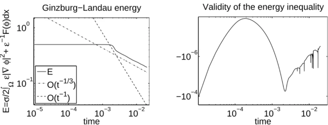
A new time discretization scheme for the numerical simulation of two-phase ow governed by a thermodynamically consistent diuse interface model is pre- sented. The scheme is consistent in the sense that it allows for a discrete in time energy inequality. An adaptive spatial discretization is proposed that conserves the energy inequality in the fully discrete setting by applying a suitable post pro- cessing step to the adaptive cycle. For the fully discrete scheme a quasi-reliable error estimator is derived which estimates the error both of the ow velocity, and of the phase eld. The validity of the energy inequality in the fully discrete setting is numerically investigated.

∗The authors gratefully acknowledge the nancial support by the Deutsche Forschungsgemeinschaft through the priority program SPP1506 entitled Transport processes at uidic interfaces.

†Fakultät für Mathematik, Universität Regensburg, 93040 Regensburg.

‡Fachbereich Mathematik, Universität Hamburg, Bundesstraÿe 55, 20146 Hamburg.

§Fachbereich Mathematik, Universität Hamburg, Bundesstraÿe 55, 20146 Hamburg.

Introduction

In the present work we propose a stable and (essentially) linear time discretization scheme for two-phase ows governed by the diuse interface model

ρ∂_tv+ ((ρv+J)· ∇)v−div(2ηDv) +∇p=µ∇ϕ+ρg ∀x∈Ω, ∀t∈I, (1) div(v) =0 ∀x∈Ω, ∀t∈I, (2)

∂_tϕ+v· ∇ϕ−div(m∇µ) =0 ∀x∈Ω, ∀t∈I, (3)

−σ∆ϕ+F⁰(ϕ)−µ=0 ∀x∈Ω, ∀t∈I, (4) v(0, x) =v₀(x) ∀x∈Ω, (5) ϕ(0, x) =ϕ₀(x) ∀x∈Ω, (6) v(t, x) =0 ∀x∈∂Ω,∀t ∈I, (7)

∇µ(t, x)·ν_Ω =∇ϕ(t, x)·ν_Ω =0 ∀x∈∂Ω,∀t ∈I, (8) where J = −_dϕ^dρm∇µ. This model is proposed in [AGG12]. Here Ω⊂ Rⁿ, n ∈ {2,3}, denotes an open and bounded domain, I = (0, T] with 0 < T < ∞ a time interval, ϕ denotes the phase eld, µ the chemical potential, v the volume averaged velocity, p the pressure, and ρ = ρ(ϕ) = ¹₂((ρ₂−ρ₁)ϕ+ (ρ₁+ρ₂)) the mean density, where 0 < ρ₁ ≤ ρ₂ denote the densities of the involved uids. The viscosity is denoted by η and can be chosen arbitrarily, fullling η(−1) = ˜η₁ and η(1) = ˜η₂, with individual uid viscosities η₁, η₂. The mobility is denoted by m = m(ϕ). The graviational force is denoted by g. By Dv = ¹₂(∇v+ (∇v)^t) we denote the symmetrized gradient. The scaled surface tension is denoted by σ and the interfacial width is proportional to . The free energy is denoted by F. For F we use a splitting F =F₊+F−, where F₊ is convex andF₋ is concave.

The above model couples the NavierStokes equations (1)(2) to the CahnHilliard model (3)(4) in a thermodynamically consistent way, i.e. a free energy inequality holds. It is the main goal to introduce and analyze an (essentially) linear time dis- cretization scheme for the numerical treatment of (1)(8), which also on the discrete level fullls the free energy inequality. This in conclusion leads to a stable scheme that is thermodynamically consistent on the discrete level.

Existence of weak solutions to system (1)(8) for a specic class of free energies F is shown in [ADG13a, ADG13b]. See also the work [Grü13], where the existence of weak solutions for a dierent class of free energies F is shown by passing to the limit in a numerical scheme. We refer to [LT98], [Boy02], [DSS07], [ADGK13], and the review [AMW98] for other diuse interface models for two-phase incompressible ow.

Numerical approaches for dierent variants of the NavierStokes CahnHilliard system have been studied in [KSW08], [Fen06], [Boy02], [AV12], [Grü13], [HHK13], [GK14] and [GLL].

This work is organized as follows. In Section 1 we derive a weak formulation of (1)(8) and formulate a time discretization scheme. In Section 2 we derive the fully discrete model and show the existence of solutions for both the time discrete, and the

fully discrete model, as well as energy inequalities, both for the time discrete model, and for the fully discrete model. In Section 3 we use the energy inequality to derive a residual based adaptive concept, and in Section 4 we numerically investigate properties of our simulation scheme.

Notation and assumptions

LetΩ⊂Rⁿ,n∈ {2,3}denote a bounded domain with boundary∂Ωand outer normal νΩ. Let I = (0, T) denote a time interval.

We use the conventional notation for Sobolev and Hilbert Spaces, see e.g. [AF03].

With L^p(Ω), 1 ≤ p ≤ ∞, we denote the space of measurable functions on Ω, whose modulus to the powerpis Lebesgue-integrable. L^∞(Ω)denotes the space of measurable functions onΩ, which are essentially bounded. Forp= 2we denote by L²(Ω)the space of square integrable functions onΩwith inner product(·,·)and normk · k. For a subset D ⊂Ω and functions f, g ∈ L²(Ω) we by (f, g)D denote the inner product of f and g restricted to D, and by kfk_D the respective norm. By W^k,p(Ω), k ≥ 1,1 ≤ p ≤ ∞, we denote the Sobolev space of functions admitting weak derivatives up to order k in L^p(Ω). If p = 2 we write H^k(Ω). The subset H₀¹(Ω) denotes H¹(Ω) functions with vanishing boundary trace.

We further set

L²₀(Ω) ={v ∈L²(Ω)|(v,1) = 0}, and with

H(div,Ω) ={v ∈H₀¹(Ω)ⁿ|(div(v), q) = 0∀q∈L²₍₀₎(Ω)}

we denote the space of all weakly solenoidal H₀¹(Ω) vector elds.

Foru∈L^q(Ω)ⁿ,q > n, and v, w∈H¹(Ω)ⁿ we introduce the trilinear form a(u, v, w) = 1

2 Z

Ω

((u· ∇)v)w dx− 1 2

Z

Ω

((u· ∇)w)v dx. (9) Note that there holds a(u, v, w) =−a(u, w, v), and especially a(u, v, v) = 0.

For the data of our problem we assume:

A1 There exists constants ρ ≥ ρ > 0, η ≥ η > 0, and m ≥ m > 0 such that the following relations are satised:

• ρ≥ρ(ϕ)≥ρ >0,

• η≥η(ϕ)≥η >0,

• m≥m(ϕ)≥m >0.

Especially we assume that the mobility is non degenerated. In addition we assume, that ρ,µ, and m are continuous.

A2 F :R→R is continuously dierentiable.

A3 F and the derivativesF₊⁰ andF₋⁰ are polynomially bounded, i.e. there existsC > 0 such that|F(x)| ≤C(1+|x|^q),|F₊⁰(x)| ≤C(1+|x|^q−1)and|F₋⁰(x)| ≤C(1+|x|^q−1) holds for some q ∈[1,4] if n= 3 and q∈[1,∞) if n = 2,

A4 F₊⁰ is Newton (sometimes called slantly) dierentiable (see e.g. [HIK03]) regarded as nonlinear operator F₊⁰ :H¹(Ω)→(H¹(Ω))^∗ with Newton derivative G satisfy- ing

(G(ϕ)δϕ, δϕ)≥0 for each ϕ∈H¹(Ω) and δϕ∈H¹(Ω).

To ensure Assumption A1 we introduce a cut-o mechanism to ensure the bounds onρ dened in Assumption A1 independently of ϕ. Note that η(ϕ) and m(ϕ) can be chosen arbitrarily fullling the stated bounds. We dene the mass density as a smooth, monotone and strictly positive functionρ(ϕ)fullling

ρ(ϕ) =







˜ ρ2−˜ρ1

2 ϕ+^{ρ˜1+ ˜}₂^ρ2 if −1−_ρ˜^ρ˜1

2−˜ρ1 < ϕ <1 + _ρ˜^ρ˜1

2−˜ρ1, const if ϕ >1 + _ρ˜^{2 ˜ρ1}

2−˜ρ1, const if ϕ <−1− _ρ˜^{2 ˜ρ1}

2−˜ρ1. For a discussion we refer to [Grü13, Remark 2.1].

Remark 1. The Assumptions A2A4 are for example fullled by the polynomial free energy

F^poly(ϕ) = σ

4 1−ϕ²2

.

Another free energy fullling these assumptions is the relaxed double-obstacle free energy given by

F^rel(ϕ) = σ

2 1−ϕ²+sλ²(ϕ)

, (10)

with

λ(ϕ) := max(0, ϕ−1) + min(0, ϕ+ 1),

where s 0 denotes the relaxation parameter. F^rel is introduced in [HHT11] as MoreauYosida relaxation of the double-obstacle free energy

F^obst(ϕ) = (_σ

2(1−ϕ²) if |ϕ| ≤1,

0 else,

which is proposed in [BE91] to model phase separation.

In the numerical examples of this work we use the free energy F ≡ F^rel. For this choice the splitting into convex and concave part reads

F₊(ϕ) =sσ

2λ²(ϕ), F−(ϕ) = σ

2(1−ϕ²).

1 The time discrete setting

In the present section we formulate our time discretization scheme that is based on a weak formulation of (1)(8) which we derive next. To begin with, note that for a suciently smooth solution (ϕ, µ, v) of (1)(8) we can rewrite (1), using the linearity of ρ, as

∂_t(ρv) +div(ρv⊗v) +div(v⊗J)−div(2ηDv) +∇p=µ∇ϕ+ρg, (11) see [AGG12, p. 14].

We also note that the term ρv+J in (1) is not solenoidal (which might lead to diculties both in the analytical and the numerical treatment) and that the trilinear form(((ρv+J)· ∇)u, w) is not anti-symmetric. To obtain a weak formulation yielding an anti-symmetric convection term we use a convex combination of (1) and (11) to dene a weak formulation. We multiply equations (1) and (11) by the solenoidal test function ¹₂w ∈ H(div,Ω), integrate over Ω, add the resulting equations and perform integration by parts. This gives

1 2

Z

Ω

(∂_t(ρv) +ρ∂_tv)w dx+ Z

Ω

2ηDv:Dw dx+a(ρv+J, v, w) = Z

Ω

µ∇ϕw+ρgw dx.

Equations (3)(4) are treated classically. This leads to

Denition 1. We call v, ϕ, µ a weak solution to (1)(8) if v(0) = v₀, ϕ(0) = ϕ₀, v(t)∈H(div,Ω)for a.e. t ∈I and

1 2

Z

Ω

(∂_t(ρv) +ρ∂_tv)w dx+ Z

Ω

2ηDv:Dw dx +a(ρv+J, v, w) =

Z

Ω

µ∇ϕw+ρgw dx ∀w∈H(div,Ω), (12) Z

Ω

(∂_tϕ+v · ∇ϕ) Φdx+ Z

Ω

m(ϕ)∇µ· ∇Φdx= 0 ∀Φ∈H¹(Ω), (13) σ

Z

Ω

∇ϕ· ∇Ψdx+ Z

Ω

F⁰(ϕ)Ψdx− Z

Ω

µΨdx= 0 ∀Ψ∈H¹(Ω), (14) is satised for almost all t ∈I.

Theorem 1. Letv, ϕ, µbe a suciently smooth solution to (12)(14). Then there holds 1

2 d dt

Z

Ω

ρ|v|²+σ|∇ϕ|²+F(ϕ)dx

=− Z

Ω

2η|Dv|²+m|∇µ|²dx+ Z

Ω

ρgv dx.

Proof. By testing (12) withw≡v, (13) withΦ≡µand (14) withΨ≡∂_tϕand adding the resulting equations the claim follows.

In [ADG13a, ADG13b] an alternative weak formulation of (1)(8) is proposed, for which the authors show existence of weak solutions.

We now introduce a time discretization which mimics the energy inequality in The- orem 1 on the discrete level. Let 0 =t₀ < t₁ < . . . < tk−1 < t_k < t_k+1 < . . . < t_M =T denote an equidistant subdivision of the interval I = [0, T] with τ_k+1−τ_k = τ. From here onwards the superscriptk denotes the corresponding variables at time instance t_k. Time integration scheme

Letϕ0 ∈H¹(Ω) and v0 ∈H(div,Ω). Initialization for k = 0:

Set ϕ⁰ =ϕ₀ and v⁰ =v₀.

Find ϕ¹ ∈ H¹(Ω), µ¹ ∈ H¹(Ω), v¹ ∈ H(div,Ω), such that for all w ∈ H(div,Ω), Φ∈H¹(Ω), andΨ∈H¹(Ω) it holds

1 τ

Z

Ω

ρ¹(v¹−v⁰)w dx+ Z

Ω

((ρ⁰v⁰+J¹)· ∇)v¹·w dx +

Z

Ω

2η¹Dv¹ :Dw dx− Z

Ω

µ¹∇ϕ¹w+ρ¹gw dx= 0 ∀w∈H(div,Ω), (15) 1

τ Z

Ω

(ϕ¹ −ϕ⁰)Φdx+ Z

Ω

(v⁰· ∇ϕ⁰)Φdx +

Z

Ω

m(ϕ⁰)∇µ¹· ∇Φdx= 0 ∀Φ∈H¹(Ω), (16) σ

Z

Ω

∇ϕ¹· ∇Ψdx− Z

Ω

µ¹Ψdx +

Z

Ω

((F+)⁰(ϕ¹) + (F−)⁰(ϕ⁰))Ψdx= 0 ∀Ψ∈H¹(Ω), (17) whereJ¹ :=−_dϕ^dρ(ϕ¹)m¹∇µ¹.

Two-step scheme for k ≥1:

Givenϕ^k−1 ∈H¹(Ω), ϕ^k ∈H¹(Ω), µ^k∈W^1,q(Ω), q > n,v^k ∈H(div,Ω),

nd v^k+1 ∈H(div,Ω),ϕ^k+1 ∈H¹(Ω), µ^k+1 ∈H¹(Ω) satisfying 1

2τ Z

Ω

ρ^kv^k+1−ρ^k−1v^k

w+ρ^k−1(v^k+1−v^k)w dx +a(ρ^kv^k+J^k, v^k+1, w) +

Z

Ω

2η^kDv^k+1 :Dw dx

− Z

Ω

µ^k+1∇ϕ^kw−ρ^kgw dx= 0 ∀w∈H(div,Ω), (18) 1

τ Z

Ω

(ϕ^k+1−ϕ^k)Φdx+ Z

Ω

(v^k+1· ∇ϕ^k)Φdx +

Z

Ω

m(ϕ^k)∇µ^k+1· ∇Φdx= 0 ∀Φ∈H¹(Ω), (19) σ

Z

Ω

∇ϕ^k+1· ∇Ψdx− Z

Ω

µ^k+1Ψdx +

Z

Ω

((F₊)⁰(ϕ^k+1) + (F−)⁰(ϕ^k))Ψdx= 0 ∀Ψ∈H¹(Ω), (20) whereJ^k:=−^dρ_dϕ(ϕ^k)m^k∇µ^k.

We note that in (18)(20) the only nonlinearity arises from F₊⁰ and thus only the equation (20) is nonlinear. Let us summarize properties of this scheme in the following remark.

Remark 2.

• The time discretization (15)(17) used in the initialization step is motivated by the time discretization in [KSW08] for the equal density case. In particular it yields a sequential coupling of the CahnHilliard and the NavierStokes systems.

Concerning the existence of a unique solution we refer to e.g. [HHK13]. From the regularity theory for the Laplace operator we have µ¹ ∈H²(Ω).

• Existence and uniqueness of a solution to the time discrete model (18)(20) is shown in Theorem 6. Using the Assumption A4 posed on F, it can be shown that Newton's method in function space can be used to compute a solution to (18)(20) using the steps from Theorem 6.

• Through the use of ρ^k−1, (18)(20) is a 2-step scheme. However, by replacing (18) with

1 2τ

Z

Ω

ρ^k+1v^k+1−ρ^kv^k

w+ρ^k(v^k+1−v^k)w dx +a(ρ^kv^k+J^k, v^k+1, w) +

Z

Ω

2ηDv^k+1 :Dw dx

− Z

Ω

µ^k+1∇ϕ^kw+ρ^kgw dx= 0 ∀w∈H(div,Ω),

one obtains an one-step scheme, which then also is nonlinear in the time dis- cretization of (12). The resulting system is analyzed in a forthcoming paper.

In [GK14] Grün and Klingbeil propose a time-discrete solver for (1)(8) which leads to strongly coupled systems for v, ϕ and p at every time step and requires a fully nonlinear solver. For this scheme Grün in [Grü13] proves an energy inequality and the existence of so called generalized solutions.

2 The fully discrete setting and energy inequalities

For a numerical treatment we next discretize the weak formulation (18)(20) in space.

We aim at an adaptive discretization of the domain Ω, and thus to have a dierent spatial discretization in every time step.

Let T^k = SN T

i=1T_i denote a conforming triangulation of Ω with closed simplices T_i, i= 1, . . . , N T and edges E_i, i= 1, . . . , N E, E^k =SN E

i=1E_i. Here k refers to the time instancetk. On T^k we dene the following nite element spaces:

V¹(T^k) ={v ∈C(T^k)|v|_T ∈P¹(T)∀T ∈ T^k}=:span{Φⁱ}^{N P}_i=1, V²(T^k) ={v ∈C(T^k)|v|_T ∈P²(T)∀T ∈ T^k},

whereP^l(S) denotes the space of polynomials up to order l dened on S. We introduce the discrete analogon to the space H(div,Ω):

H(div,T^k) = {v ∈ V²(T^k)ⁿ|(divv, q) = 0∀q∈ V¹(T^k)∩L²₍₀₎(Ω), v|∂Ω = 0}

:=span{bⁱ}^{N F}_i=1,

We further introduce a H¹-stable projection operator P^k :H¹(Ω) → V¹(T^k) satis- fying

kP^kvk_L^p_(Ω)≤ kvk_L^p_(Ω) and k∇P^kvk_L^r_(Ω) ≤ k∇vk_L^r_(Ω)

for v ∈ H¹(Ω) with r ∈ [1,2] and p ∈ [1,6) if n = 3, and p ∈ [1,∞) if n = 2. Possible choices are the Clément operator ([Clé75]) or, by restricting the preimage to C(Ω)∩H¹(Ω), the Lagrangian interpolation operator.

Using these spaces we state the discrete counterpart of (18)(20):

Let k ≥ 1, given ϕ^k−1 ∈ V¹(T^k−1), ϕ^k ∈ V¹(T^k), µ^k ∈ V¹(T^k), v^k ∈ H(div,T^k), nd v^k+1_h ∈ H(div,T^k+1), ϕ^k+1_h ∈ V¹(T^k+1), µ^k+1_h ∈ V¹(T^k+1) such that for all w ∈ H(div,T^k+1), Φ∈ V¹(T^k+1), Ψ∈ V¹(T^k+1) there holds:

1

2τ(ρ^kv_h^k+1−ρ^k−1v^k+ρ^k−1(v_h^k+1−v^k), w) +a(ρ^kv^k+J^k, v_h^k+1, w)

+(2η^kDv^k+1_h , Dw)−(µ^k+1_h ∇ϕ^k+ρ^kg, w) = 0, (21) 1

τ(ϕ^k+1_h − P^k+1ϕ^k,Φ) + (m(ϕ^k)∇µ^k+1_h ,∇Φ) + (v^k+1_h ∇ϕ^k,Φ) = 0, (22) σ(∇ϕ^k+1_h ,∇Ψ) + (F₊⁰(ϕ^k+1_h ) +F₋⁰(P^k+1ϕ^k),Ψ)−(µ^k+1_h ,Ψ) = 0, (23)

where ϕ⁰ = P ϕ₀ denotes the L² projection of ϕ₀ in V¹(T⁰), v⁰ = P^Lv₀ denotes the Leray projection ofv₀ inH(div,T⁰) (see [CF88]), andϕ¹_h, µ¹_h, v_h¹ are obtained from the fully discrete variant of (15)(17).

2.1 Existence of solution to the fully discrete system

We next show the existence of a unique solution to the fully discrete system (21)(23).

Theorem 2. There exist v_h^k+1 ∈ H(div,T^k+1), ϕ^k+1_h ∈ V¹(T^k+1), µ^k+1_h ∈ V¹(T^k+1) solving (21)(23).

Proof. By testing (22) with Φ ≡ 1, integration by parts in (v^k+1_h ∇ϕ^k,1) and using v_h^k+1 ∈H(div,T^k+1) we obtain

(ϕ^k+1_h ,1) = (P^k+1ϕ^k,1).

We dene α= _|Ω|¹ R

ΩP^k+1ϕ^kdx and set

V₍₀₎ :={v_h ∈ V¹(T^k+1) | (v_h,1) = 0}.

Thenz^k+1 :=ϕ^k+1−αfullls z^k+1 ∈V₍₀₎. In the following we use z^k+1 as unknown for the phase eld, since the mean value of ϕ is xed. In addition we introduce y^k+1 :=

µ^k+1_h −_|Ω|¹ R

µ^k+1_h dxand require (22)(23) preliminarily only for test functions with zero mean value.

We dene

X =H(div,T^k+1)×V₍₀₎×V₍₀₎, with the inner product

((v₁, y₁, z₁),(v₂, y₂, z₂))_X := (Dv₁, Dv₂) + (∇y₁,∇y₂) + (∇z₁,∇z₂),

and norm k · k²_X = (·,·)_X. It follows from the inequalities of Korn and Poincaré that (·,·)_X indeed forms an inner product onX. For (v, y, z)∈X we dene

(G(v, y, z),(v, y, z))_X :=

1

2(ρ^k+ρ^k−1)v−ρ^k−1v^k, v

+τ a(ρ^kv^k+J^k, v, v) +τ(2η^kDv, Dv)−τ(y∇ϕ^k, v)−τ(ρ^kg, v)

+ (z− P^k+1ϕ^k, y) +τ(m(ϕ^k)∇y,∇y) +τ(v∇ϕ^k, y) +σ(∇z,∇z) + (F₊⁰(z+α) +F₋⁰(P^k+1ϕ^k), z)−(y, z).

Now we show(G(v, y, z),(v, y, z))X >0fork(v, y, z)kX large enough and thatGsatises the supposition of [Tem77, Lem. II.1.4]. It then follows from [Tem77, Lem. II.1.4], that Gadmits a root (v^∗, y^∗, z^∗)∈X.

The function Gis obviously continuous. We now estimate (G(v, y, z),(v, y, z))_X ≥ρ(v, v) + 2τ η(Dv, Dv)

+τ m(∇y,∇y) +σ(∇z,∇z) + (F₊⁰(z+α), z)

−(ρ^k−1v^k, v)−τ(ρ^kg, v)−(P^k+1ϕ^k, y) + (F₋⁰(P^k+1ϕ^k), z).

Using the convexity ofF+, which implies that F₊⁰ is monotone, we obtain (24)

(F₊⁰(z+α), z) = (F₊⁰ (z+α)−F₊⁰(α), z) + (F₊⁰(α), z)≥(F₊⁰(α), z).

By using Hölder's and Poincaré's inequality in (24) we obtain (G(v, y, z),(v, y, z))_X >0

fork(v, y, z)k_X ≥RifRis large enough. Now [Tem77, Lem. II.1.4] implies the existence of (v^∗, y^∗, z^∗) ∈X such that G(v^∗, y^∗, z^∗) = 0. Dening (v, µ, ϕ) = (v^∗, y^∗+β, z^∗+α) withβ such that(β,1) = (F₊⁰(ϕ) +F₋⁰(P^k+1ϕ^k),1)we obtain that(v, µ, ϕ)solves (21) (23).

Remark 3. Note that we do not need that the variables from old time instances are dened on the mesh used on the current time instance. We further do not need any smallness requirement on the mesh size h or on the time step length τ.

Theorem 3. Let(ϕ^k+1_h , µ^k+1_h , v_h^k+1) be a solution to (21)(23). Then fork ≥1: 1

2 Z

Ω

ρ^k v_h^k+1

2 dx+σ 2

Z

Ω

|∇ϕ^k+1_h |²dx+ Z

Ω

F(ϕ^k+1_h )dx +1

2 Z

Ω

ρ^k−1|v^k+1_h −v^k|²dx+ σ 2

Z

Ω

|∇ϕ^k+1_h − ∇P^k+1ϕ^k|²dx +τ

Z

Ω

2η^k|Dv_h^k+1|²dx+τ Z

Ω

m^k|∇µ^k+1_h |²dx

≤ 1 2

Z

Ω

ρ^k−1 v^k

2 dx+ σ 2

Z

Ω

|∇P^k+1ϕ^k|²dx+ Z

Ω

F(P^k+1ϕ^k)dx+τ Z

Ω

ρ^kgv_h^k+1. (25) Proof. We have

1

2 ρ^kv_h^k+1−ρ^k−1v^k

·v_h^k+1+1

2ρ^k−1 v_h^k+1−v^k

·v_h^k+1

= 1 2ρ^k

v_h^k+1

2+1 2ρ^k−1

v_h^k+1−v^k

2−1 2ρ^k−1

v^k

2, (26)

∇ϕ^k+1_h · ∇ϕ^k+1_h − ∇ϕ^k

=1

2|∇ϕ^k+1_h |²− 1

2|∇ϕ^k|²+1

2|∇ϕ^k+1_h − ∇ϕ^k|², (27)

and since F₊ is convex and F− is concave,

F₊(ϕ^k+1_h )−F₊(ϕ^k)≤F₊⁰(ϕ^k+1_h )(ϕ^k+1_h −ϕ^k), (28) F₋(ϕ^k+1_h )−F₋(ϕ^k)≤F₋⁰(ϕ^k)(ϕ^k+1_h −ϕ^k). (29) The inequality is now obtained from testing (18) with v_h^k+1, (19) with µ^k+1_h , (20) with (ϕ^k+1_h − P^k+1ϕ^k)/τ, and adding the resulting equations. This leads to

1

2τ(ρ^kv_h^k+1−ρ^k−1v^k, v_h^k+1) + 1

2τ(ρ^k−1(v_h^k+1−v^k), v^k+1_h ) +a(ρ^kv+J^k, v_h^k+1, v_h^k+1) + (2η^kDv_h^k+1 :Dv_h^k+1)−(µ^k+1_h ∇ϕ^k, v^k+1_h ) +1

τ(ϕ^k+1_h − P^k+1ϕ^k, µ^k+1_h ) + (v_h^k+1∇ϕ^k, µ^k+1_h ) + (m^k∇µ^k+1_h ,∇µ^k+1_h ) +σ1

τ(∇ϕ^k+1_h ,∇(ϕ^k+1_h − P^k+1ϕ^k))− 1

τ(µ^k+1_h , ϕ^k+1_h − P^k+1ϕ^k) +1

τ(F₊⁰(ϕ^k+1_h ), ϕ^k+1_h − P^k+1ϕ^k) + 1

τ(F₋⁰(ϕ^k), ϕ^k+1_h − P^k+1ϕ^k)

−(ρ^kg, v^k+1_h ) = 0.

The equalities (26) and (27) and the inequalities (28) and (29) now imply 1

2τ Z

Ω

ρ^k|v^k+1_h |²+ρ^k−1|v_h^k+1−v^k|² −ρ^k−1|v^k|² dx +

Z

Ω

2η^k|Dv^k+1_h |²dx+ Z

Ω

m^k|∇µ^k+1_h |²dx +σ

2τ Z

Ω

|∇ϕ^k+1_h |²dx− σ 2τ

Z

Ω

|∇P^k+1ϕ^k|²dx+ σ 2τ

Z

Ω

|∇ϕ^k+1_h − ∇P^k+1ϕ^k|²dx +1

τ Z

Ω

F(ϕ^k+1_h )−F(P^k+1ϕ^k) dx−

Z

Ω

ρ^kgv_h^k+1dx≤0, which is the claim.

Theorem 4. System (21)(23) admits a unique solution.

Proof. Assume there exist two dierent solutions to (21)(23) denoted by (v¹, ϕ¹, µ¹) and (v², ϕ², µ²). We show that the dierence v =v¹ −v², ϕ =ϕ¹−ϕ², µ =µ¹ −µ² is zero.

After inserting the two solutions into (21)(23) and substracting the two sets of equations we perform the same steps as for the derivation of the discrete energy esti- mate, Theorem 3, and obtain

0 =1 2

Z

Ω

(ρ^k+ρ^k−1)v²dx+ 2τ Z

Ω

η^k|Dv|²dx +τk√

m^k∇µk² +σk∇ϕk²+ F₊⁰(ϕ¹)−F₊⁰(ϕ²), ϕ¹−ϕ² .

Since all these terms are non negative we obtain 1

2 Z

Ω

(ρ^k+ρ^k−1)v²dx=0,

Z

Ω

η^k|Dv|²dx=0, k∇µk² =0, k∇ϕk² =0.

Since bothη(·)andρ(·)are strictly positive by Assumption A1 we concludekvk_H¹_(Ω)ⁿ = 0and thus the uniqueness of the velocity eld.

By testing (22) by Φ ≡ 1 we obtain (ϕ¹,1) = (ϕ²,1) = (P^k+1ϕ^k,1) and thus (ϕ¹−ϕ²,1) = 0. Poincaré-Friedrichs inequality then yieldskϕk_H¹_(Ω) = 0, and thus the uniqueness of the phase eld.

Last we directly obtain that the chemical potential is unique up to a constant.

By testing (23) with Ψ ≡ 1 and inserting the two solutions we obtain (µ¹−µ²,1) = (F₊⁰(ϕ¹)−F₊⁰(ϕ²),1) = 0 and thus kµk_H¹_(Ω) = 0, again by using Poincaré-Friedrichs inequality.

Theorem 3 estimates the Ginzburg Landau energy of the current phase eld ϕ^k+1 against the Ginzburg Landau energy of the projection of the old phase eld P^k+1(ϕ^k). Our aim is to obtain global in time inequalities estimating the energy of the new phase eld against the energy of the old phase eld at each time step. For this purpose let us state an assumption that later will be justied.

Assumption 1. Let ϕ^k ∈ V¹(T^k) denote the phase eld at time instance t_k. Let P^k+1ϕ^k ∈ V¹(T^k+1) denote the projection of ϕ^k in V¹(T^k+1). We assume that there holds

F(P^k+1ϕ^k) + 1

2σ|∇P^k+1ϕ^k|² ≤F(ϕ^k) + 1

2σ|∇ϕ^k|². (30) This assumption means, that the Ginzburg Landau energy is not increasing through projection. Thus no energy is numerically produced.

Assumption 1 is in general not fullled for arbitrary sequences (T^k+1) of triangula- tions. To ensure (30) we add a post processing step to the adaptive space meshing, see Section 3.

Theorem 5. Assume that for every k = 0,1, . . . Assumption 1 holds. Then for every

1≤k < l we have 1

2(ρ^k−1_h v^k_h, v^k_h)+

Z

Ω

F(ϕ^k_h)dx+ 1

2σ(∇ϕ^k_h,∇ϕ^k_h) +τ

l−1

X

m=k

(ρ^mg, v_h^m+1)

≥ 1

2(ρ^l−1v_h^l, v_h^l) + Z

Ω

F(ϕ^l_h)dx+1

2σ(∇ϕ^l_h,∇ϕ^l_h) +

l−1

X

m=k

(ρ^m−1(v_h^m+1−v^m_h),(v_h^m+1−v^m_h))

+τ

l−1

X

m=k

(2η^mDv_h^m+1, Dv_h^m+1)

+τ

l−1

X

m=k

(m(ϕ^m_h)∇µ^m+1_h ,∇µ^m+1_h )

+ 1 2σ

l−1

X

m=k

(∇ϕ^m+1_h − ∇P^m+1ϕ^m_h,∇ϕ^m+1_h − ∇P^m+1ϕ^m_h).

Proof. The stated result is obtained immediately from the energy estimate over one time step (3) together with the Assumption 1.

Remark 4. We note that using Φ = 1 in (22) and using integration by parts only delivers (ϕ^k+1_h ,1) = (P^k+1ϕ^k,1) instead of (ϕ^k+1_h ,1) = (ϕ^k,1). If we use the quasi interpolation operator Q^k+1 introduced by Carstensen in [Car99] for our generic pro- jectionP^k+1, we would obtain (ϕ^k+1_h ,1) = (ϕ^k,1)since Q^k+1 preserves the mean value, i.e. (ϕ^k+1_h ,1) = (Q^k+1ϕ^k,1) ∀ϕ∈L¹(Ω).

On the other hand if we use Lagrange interpolation I^k+1 we have |(I^k+1ϕ^k,1)_T − (ϕ^k,1)_T| ≤Ch³_Tkϕ^kk_T, and the deviation of (I^k+1ϕ^k,1) from (ϕ^k,1) remaines small if we use bisection as renement strategy, since thenI^k+1ϕ^k∈ V¹(T^k+1)andϕ^k∈ V¹(T^k) only dier on coarsened patches.

2.2 Existence of a solution to the time discrete system

Now we have shown that there exists a unique solution to (21)(23). The energy inequality can be used to obtain uniform bounds on the solution and will be used to obtain a solution to the time discrete system (18)(20) by a Galerkin method.

Theorem 6. Letv^k∈H(div,Ω), ϕ^k−1 ∈H¹(Ω), ϕ^k∈H¹(Ω), andµ^k ∈W^1,q(Ω), q > n be given data. Then there exists a weak solution to (18)(20). Moreover,ϕ^k+1 ∈H²(Ω) and µ^k+1 ∈H²(Ω) holds.

Proof. We proceed as follows. We construct a sequence of meshes (T_l^k+1)l→∞ with gridsizeh_l ^l→∞−→0. We show that the sequence (v^k+1_l , ϕ^k+1_l , µ^k+1_l )of unique and discrete

solutions to (21)(23) is bounded independently of l, and thus a weakly convergent subsequence exists which we show to converge to a weak solution of (18)(20).

Let us start with dening the sequence of meshes. Let T₀^k+1 = T^k+1 and T_l+1^k+1, l = 0,1, . . ., be obtained from T_l^k+1 by bisection of all triangles. The projection onto T_l^k+1 we denote byP_l^k+1.

From the discrete energy inequality (25) we obtain 1

2 Z

Ω

ρ^k v_l^k+1

2 dx+ σ 2

Z

Ω

|∇ϕ^k+1_l |²dx+ Z

Ω

F(ϕ^k+1_l )dx +1

2 Z

Ω

ρ^k−1|v_l^k+1−v^k|²dx+σ 2

Z

Ω

|∇ϕ^k+1_l − ∇P_l^k+1ϕ^k|²dx +τ

Z

Ω

2η^k|Dv_l^k+1|²dx+τ Z

Ω

m^k|∇µ^k+1_l |²dx

≤ 1 2

Z

Ω

ρ^k−1 v^k

2 dx+ σ 2

Z

Ω

|∇P_l^k+1ϕ^k|²dx+ Z

Ω

F(P_l^k+1ϕ^k)dx+τ Z

Ω

ρ^kgv^k+1_l . We have the stability of the projection operator and thus

Z

Ω

|∇P_l^k+1ϕ^k|²dx≤ k∇ϕ^kk²_L2(Ω).

Due to Assumption A3 onF there exists a constant C >0 such that Z

Ω

F(P_l^k+1ϕ^k)dx≤C Z

Ω

|P_l^k+1ϕ^k|^q+ 1dx

≤C

kP_l^k+1ϕ^kk^q_Lq(Ω)+ 1

≤C

kϕ^kk^q_Lq(Ω)+ 1 ,

where we again use theL^q-stability of the projection operator together with the Sobolev embeddingH¹(Ω),→L^q(Ω) with q as in Assumption A3. By using Hölder's inequality and Young's inequality we further have

τ Z

Ω

ρ^kgv_l^k+1dx≤τ Z

Ω

ρ^k|g|²dx

1/2Z

Ω

ρ^k|v^k+1_l |²dx 1/2

≤τ² Z

Ω

ρ^k|g|²dx+ 1 4

Z

Ω

ρ^k|v_l^k+1|²dx

Since ρ^k−1 > 0, ρ^k > 0, η^k > 0, and m^k > 0 by Assumption A1 we obtain that kv_l^k+1k_H¹_(Ω), k∇ϕ^k+1_l k and k∇µ^k+1_l k are uniformly bounded independend of l.

By inserting Φ ≡ 1 in (22) we obtain (P_l^k+1ϕ^k,1) = (ϕ^k+1_l ,1) and by Poincaré- Friedrichs inequality thus

kϕ^k+1_l k_H¹_(Ω) ≤C k∇ϕ^k+1_l k+ (P_l^k+1ϕ^k,1)

≤C k∇ϕ^k+1_l k+kP_l^k+1ϕ^kk

≤C k∇ϕ^k+1_l k+kϕ^kk .

Thuskϕ^k+1_l k_H¹_(Ω) is uniformly bounded.

By inserting Ψ≡1 in (23) we obtain(µ^k+1_l ,1) = (F₊⁰(ϕ^k+1_l ) +F₋⁰ (P_l^k+1ϕ^k),1). Due to the Assumption A3 onF₊⁰ the rst part can be bounded byC(kϕ^k+1_l k^q_Lq(Ω)+ 1)which is bounded by Sobolev embedding. Also due to Assumption A3 on F− and due to the L^q stability ofP_l^k+1 the second part can be bounded byC(kϕ^kk^q_Lq(Ω)+ 1). Thus, by the same arguments as kϕ^k+1_l k_H¹_(Ω), also kµ^k+1_l k_H¹_(Ω) is uniformly bounded.

Consequently there exist v ∈ H₀¹(Ω)ⁿ, ϕ ∈ H¹(Ω), µ ∈ H¹(Ω) and a subsequence l_i such thatv^k+1_l

i * v inH₀¹(Ω)ⁿ, ϕ^k+1_l

i * ϕ in H¹(Ω), µ^k+1_l

i * µ in H¹(Ω) for l_i → ∞. We show that this triple of functions indeed is a weak solution to (18)(20). Inserting the sequence into (18)(20) yields

1 2τ

Z

Ω

ρ^kv_l^k+1

i −ρ^k−1v^k

w+ρ^k−1(v^k+1_l

i −v^k)w dx +a(ρ^kv^k+J^k, v_l^k+1

i , w) + Z

Ω

2η^kDv_l^k+1

i :Dw dx

− Z

Ω

µ^k+1_l

i ∇ϕ^kw+ρ^kgw dx= 0, ∀w∈H(div,Ω) (31) τ⁻¹

Z

Ω

(ϕ^k+1_l

i −ϕ^k)Φdx+

Z

Ω

(v^k+1_l

i · ∇ϕ^k)Φdx

+ Z

Ω

m(ϕ^k)∇µ^k+1_l

i · ∇Φdx= 0, ∀Φ∈H¹(Ω) (32)

σ Z

Ω

∇ϕ^k+1_l

i · ∇Ψdx−

Z

Ω

µ^k+1_l

i Ψdx

+ Z

Ω

((F₊)⁰(ϕ^k+1_l

i ) + (F−)⁰(ϕ^k))Ψdx= 0.∀Ψ∈H¹(Ω). (33) Now there holds

1 2τ

Z

Ω

ρ^k+ρ^k−1 v_l^k+1

i w dx≤ 1

τρkv_l^k+1

i k_L²_(Ω)kwk_L²_(Ω) and thus _2τ¹ R

Ω ρ^k+ρ^k−1

w· dx∈(H₀¹(Ω)ⁿ)^∗ yielding 1

2τ Z

Ω

ρ^k+ρ^k−1 v_l^k+1

i w dx → 1

2τ Z

Ω

ρ^k+ρ^k−1

vw dx.

Since µ^k ∈W^1,q(Ω), q > n there holds J^k ∈L^q(Ω) and thus by Sobolev embedding we obtain

Z

Ω

ρ^kv^k+J^k

· ∇ v_l^k+1

i

w dx

≤Ck ρ^kv^k+J^k

wkk∇v^k+1_l

i k,

Z

Ω

ρ^kv^k+J^k

· ∇ w

v_l^k+1

i dx

≤Ck ρ^kv^k+J^k

∇ wk

L

2q q+2kv_l^k+1

i k

L

2q q−2,

and thusa(ρ^kv^k+J^k,·, w)∈(H₀¹(Ω)ⁿ)^∗. This gives a(ρ^kv^k+J^k, v^k+1_l

i , w)→a(ρ^kv^k+J^k, v, w)

The convergence of the remaining terms can be concluded in a similar manner.

Since ϕ^k+1_l

i * ϕ inH¹(Ω) there exists a subsequence, again denoted by l_i such that ϕ^k+1_l

i →ϕ inL^q(Ω), q as in Assumption A3. From Assumption A3 and the dominated convergence theorem we thus obtain

Z

Ω

F₊⁰(ϕ^k+1_l

i )Ψdx →

Z

Ω

F₊⁰(ϕ)Ψdx.

Next we show the weak solenoidality of v. To begin with we note that every q ∈ L²₍₀₎(Ω) can be approximated by a sequence (ql)l∈N ⊂ V¹(T_l^k+1)∩L²₍₀₎(Ω), so that for every ξ > 0 an index N_ξ exists, such that kq−q_lk ≤ ξ for l ≥ N_ξ. Now we have for arbitraryq ∈L²₍₀₎(Ω)

|(div v, q)| ≤ |(divv, q−q_l)|+|(div v−div v_li, q_l)|+|(div v_li, q_l)|.

Letξ >0be given. For the rst addend we have|(div v, q−q_l)| ≤ kdiv vkkq−q_lk ≤Cξ forl ≥N_ξ.

Since the sequence q_l is dened on the same hierarchy of meshes as v_l we may restrict q_l to the subsequence l_i and obtain that both q_li and v_li are dened on the same meshes. We set k := min{l_i|l_i ≥ N_ξ}. Now we have (div v_li, q_k) = 0 for l_i ≥ k, since then q_k ∈ V¹(T_l^k+1

i ), i.e. the third addend vanishes. By choosing l_i so large that

|(div v −divv_li, q_k)| ≤ Cξ holds by weak convergence of v_li, the weak solenoidality of v is shown, sinceξ >0 is chosen arbitrarily.

Thus the triplev, ϕ, µ indeed is a weak solution.

It remains to obtain the stated higher regularity for µ^k+1 and ϕ^k+1. This directly follows by regularity results for the Laplacian, see [EG04, Thm. 3.10]. Since µ^k+1− F₊⁰ (ϕ^k+1)−F₋⁰(ϕ^k) ∈ L²(Ω) it follows that ϕ^k+1 ∈ H²(Ω) and thus, since we have τ⁻¹(ϕ^k+1−ϕ^k) +v^k+1∇ϕ^k ∈L²(Ω), also µ^k+1 ∈H²(Ω).

The uniqueness of the solution follows by the same steps as the uniqueness of the discrete solutions, see Theorem 4. Like the fully discrete scheme, also the time-discrete scheme fullls an energy inequality.

Theorem 7. Letϕ^k+1, µ^k+1, v^k+1 be a solution to (18)(20). Then the following energy

inequality holds.

1 2

Z

Ω

ρ^k v^k+1

2 dx+σ 2

Z

Ω

|∇ϕ^k+1|²dx+ Z

Ω

F(ϕ^k+1)dx +1

2 Z

Ω

ρ^k−1|v^k+1−v^k|²dx+ σ 2

Z

Ω

|∇ϕ^k+1− ∇ϕ^k|²dx +τ

Z

Ω

2η^k|Dv^k+1|²dx+τ Z

Ω

m^k|∇µ^k+1|²dx

≤ 1 2

Z

Ω

ρ^k−1 v^k

2 dx+ σ 2

Z

Ω

|∇ϕ^k|²dx+ Z

Ω

F(ϕ^k)dx.+ Z

Ω

ρ^kgv^k+1

Proof. The inequality is obtaind from testing (18) withv^k+1, (19) with µ^k+1, (20) with (ϕ^k+1−ϕ^k)/τ and using the same arguments as in the proof for Theorem 3.

Remark 5. Let F denote the relaxed double-obstacle free energy introduced in Re- mark 1, with relaxation parameters. Let(v_s, ϕ_s, µ_s)s∈R denote the sequence of solutions of (18)(20) for a sequence(s_l)l∈N. From the linearity of (18) and [HHT11, Prop. 4.2]

it follows, that there exists a subsequence, still denoted by (vs, ϕs, µs)s∈R, such that (v_s, ϕ_s, µ_s)_s∈R→(v^∗, ϕ^∗, µ^∗) in H¹(Ω),

where (v^∗, ϕ^∗, µ^∗) denotes the solution of (18)(20), whereF^obst, denoted in Remark 1, is chosen as free energy. Especially |ϕ^∗| ≤ 1 holds. In the following argumentation we concentrate on the phase eld only. From the regularity ϕ_s ∈ H²(Ω) together with a-priori estimates on the solution of the Poisson problem and the energy inequality of Theorem 7, we obtain the existence of a strongly convergent subsequence ϕ_s⁰ → ϕ^∗ in C^0,α(Ω), where we use the compact embedding H²(Ω),→C^0,α(Ω) for 2α <4−n.

Thus for s large enough we have |ϕ_s| ≤1 +θ with θ arbitrarily small. Currently we are not able to quantify how large s has to be chosen in dependence of θ to guarantee this bound. Therefore we use the cut-o procedure described before Remark 1.

3 The A-Posteriori Error Estimation

For an ecient solution of (21)(23) we next describe an a-posteriori error estimator based mesh renement scheme that is reliable and ecient up to terms of higher order and errors introduced by the projection. We also describe how Assumption 1 on the evolution of the free energy, given in (25), under projection is fullled in the discrete setting.

Let us briey comment on available adaptative concepts for the spatial discretization of CahnHilliard NavierStokes systems. Heuristic approaches exploiting knowledge of the location of the diuse interface can be found in [KSW08, BBG11, AV12, GK14]. In [HHK13] a fully adaptive, reliable and ecient, residual based error estimator for the CahnHilliard part in the CahnHilliard NavierStokes system is proposed, which ex- tends the results of [HHT11] for CahnHilliard to CahnHilliard NavierStokes systems