Fate of terrestrial organic carbon and associated CO2

(1)

www.biogeosciences.net/13/691/2016/

doi:10.5194/bg-13-691-2016

Fate of terrestrial organic carbon and associated CO ₂ and CO emissions from two Southeast Asian estuaries

D. Müller^1,2, T. Warneke¹, T. Rixen^2,3, M. Müller⁴, A. Mujahid⁵, H. W. Bange⁶, and J. Notholt^1,7

1Institute of Environmental Physics, University of Bremen, Otto-Hahn-Allee 1, 28359 Bremen, Germany

2Leibniz Center for Tropical Marine Ecology, Fahrenheitstr. 6, 28359 Bremen, Germany

3Institute of Geology, University of Hamburg, Bundesstr. 55, 20146 Hamburg, Germany

4Swinburne University of Technology, Faculty of Engineering, Computing and Science, Jalan Simpang Tiga, 93350 Kuching, Sarawak, Malaysia

5Department of Aquatic Science, Faculty of Resource Science and Technology, University Malaysia Sarawak, 94300 Kota Samarahan, Sarawak, Malaysia

6GEOMAR Helmholtz Centre for Ocean Research Kiel, Düsternbrooker Weg 20, 24105 Kiel, Germany

7MARUM Center for Marine Environmental Sciences, University of Bremen, Leobener Str., 28359 Bremen, Germany Correspondence to: D. Müller (dmueller@iup.physik.uni-bremen.de)

Received: 4 May 2015 – Published in Biogeosciences Discuss.: 5 June 2015

Revised: 6 January 2016 – Accepted: 14 January 2016 – Published: 4 February 2016

Abstract. Southeast Asian rivers convey large amounts of organic carbon, but little is known about the fate of this terrestrial material in estuaries. Although Southeast Asia is, by area, considered a hotspot of estuarine carbon dioxide (CO2) emissions, studies in this region are very scarce. We measured dissolved and particulate organic carbon, as well as CO₂partial pressures and carbon monoxide (CO) concentrations in two tropical estuaries in Sarawak, Malaysia, whose coastal area is covered by carbon-rich peatlands. We sur- veyed the estuaries of the rivers Lupar and Saribas during the wet and dry season, respectively. Carbon-to-nitrogen ratios suggest that dissolved organic matter (DOM) is largely of terrestrial origin. We found evidence that a large fraction of this carbon is respired. The median pCO₂ in the estuaries ranged between 640 and 5065 µatm with little seasonal variation. CO2fluxes were determined with a floating chamber and estimated to amount to 14–268 mol m⁻²yr⁻¹, which is high compared to other studies from tropical and subtropical sites. Estimates derived from a merely wind-driven turbulent diffusivity model were considerably lower, indicating that these models might be inappropriate in estuaries, where tidal currents and river discharge make an important contribution to the turbulence driving water–air gas exchange. Although an observed diurnal variability of CO concentrations suggested that CO was photochemically pro-

duced, the overall concentrations and fluxes were relatively moderate (0.4–1.3 nmol L⁻¹and 0.7–1.8 mmol m⁻²yr⁻¹) if compared to published data for oceanic or upwelling systems. We attributed this to the large amounts of suspended matter (4–5004 mg L⁻¹), limiting the light penetration depth and thereby inhibiting CO photoproduction. We concluded that estuaries in this region function as an efficient filter for terrestrial organic carbon and release large amounts of CO₂ to the atmosphere. The Lupar and Saribas rivers deliver 0.3±0.2 Tg C yr⁻¹ to the South China Sea as organic carbon and their mid-estuaries release approximately 0.4±0.2 Tg C yr⁻¹into the atmosphere as CO₂.

1 Introduction

Estuaries are net heterotrophic systems (Duarte and Prairie, 2005; Cole et al., 2007) and act as a source of carbon dioxide (CO₂) to the atmosphere, releasing 150 Tg C annually (Laruelle et al., 2013). Southeast Asia is considered one of the hotspot regions of aquatic CO₂ emissions to the atmosphere (Regnier et al., 2013), because many Southeast Asian rivers exhibit high organic carbon concentrations (Alkhatib et al., 2007; Moore et al., 2011, 2013; Müller et al., 2015). It has been estimated that Indonesian rivers alone account for

(2)

10 % of the dissolved organic carbon (DOC) exported to the ocean globally (Baum et al., 2007), which was attributed to the presence of tropical peatlands. Southeast Asian peatlands store 68.5 Gt carbon (Page et al., 2011) and represent a globally important carbon pool. DOC concentrations in South- east Asian peat-draining rivers range up to 5667 µmol L⁻¹ (Moore et al., 2013). Although a small fraction of this DOC is respired in the river and released to the atmosphere as CO₂, the larger part is transported downstream (Müller et al., 2015), ultimately reaching the estuary and the coastal ocean.

So far, the fate of this carbon fraction remains unclear, and data particularly in this region are scarce.

Peat-derived organic matter consists mainly of lignin and its derivates (Andriesse, 1988) and is thus relatively recalcitrant to degradation. In addition, short water residence times constrain organic matter decomposition (Müller et al., 2015).

However, high organic carbon loads and high temperatures suggest high microbial activity both in the water column and in the sediments, leading to high decomposition rates.

Additionally, photodegradation was proposed as an important removal mechanism for terrestrial organic matter in the ocean (Miller and Zepp, 1995). Chromophoric dissolved organic matter (CDOM) absorbs light, mainly in the UV region. The absorbed photons initiate abiotic photochemical reactions, during which carbon monoxide (CO) and CO₂ are produced (Stubbins, 2001), with the CO2production be- ing 14 to 20 times larger than CO production (Vähätalo, 2010). Photochemistry might be of particular importance in estuaries (Ohta et al., 2000), where dissolved organic matter (DOM) is largely of terrestrial origin. Terrestrial CDOM was found to be more efficient in producing CO than marine CDOM (Zhang et al., 2006), making estuaries a significant source of CO to the atmosphere (Valentine and Zepp, 1993).

Ultimately, recalcitrant terrestrial organic matter might be subject to photobleaching (Vähätalo, 2010), increasing its bioavailability to the heterotrophic community.

In order to investigate whether and how terrestrial organic carbon is processed in tropical estuaries, we studied organic carbon, dissolved CO₂and CO in two Malaysian estuaries, both of which receive terrestrial carbon from rivers draining a catchment that is partially covered by peat.

2 Materials and methods 2.1 Study area

Sarawak is Malaysia’s largest state and is located in the northwest of the island of Borneo, which is divided between Indonesia, Brunei and Malaysia. It is separated from peninsu- lar Malaysia by the South China Sea. Sarawak has a tropical climate. The mean annual air temperature in Sarawak’s cap- ital Kuching (1.56^◦N, 110.35^◦E) is 26.1^◦C (average 1961–

1990, DWD, 2007). Rainfall is high throughout the year, but

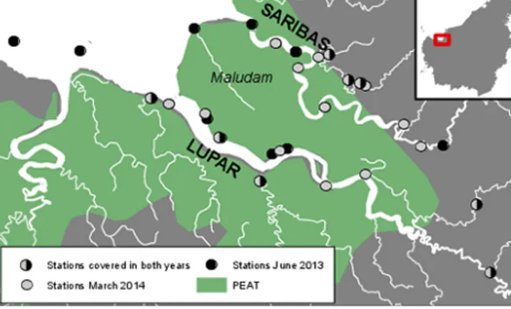
Figure 1. Map of the study area. The stations are indicated by the grey and black dots; peat soils (histosols) are indicated in green (as of FAO, 2009).

pronounced during the northeastern monsoon, which occurs between November and February.

Our study focused on two macrotidal estuaries in western Sarawak (tidal range 3–4 m). The coastal area of western Sarawak is covered by peatlands. The largest peat dome is found on the Maludam peninsula. It is rainwater-fed and covered by dense peat swamp forest, which has been protected ever since Maludam was gazetted as a national park in 2000.

The peninsula is enclosed by the rivers Lupar and Saribas (Fig. 1), which originate in upland areas. Six channels from the Maludam peat swamp forest drain into the Lupar estuary and six into the Saribas, respectively (Kselik and Liong, 2004). With reference to their catchment areas, the peat coverage in the Lupar and Saribas basins is 30.5 and 35.5 %, respectively (FAO, 2009), whereas the peat is located very close to the coast (Fig. 1). The catchment sizes are 6558 km² (Lupar) and 1943 km²(Saribas) (Lehner et al., 2006).

Sampling was performed during two ship cruises in 2013 and 2014. The 2013 cruise took place in June (18–23 June) during the dry season. The 2014 cruise was performed in March (10–19 March), right after the end of the monsoon season. We sampled 20 stations in 2013 and 23 stations in 2014 (Fig. 1). Here, we report the data separately for the lower (salinity >25), middle (salinities 2–25) and upper (salinity<2) estuaries. In 2014, we went further upstream than in 2013. Therefore, when it comes to the mid-estuaries, we report medians for the “2013 spatial extent”, i.e., refer to the spatial coverage of 2013.

2.2 Discharge and flow velocity

We estimated river discharge (Q) from the difference between precipitation (P) and evapotranspiration (ET). Precip- itation was taken from NOAA NCEP Reanalysis data set for the nearest upstream grid (0.95^◦N, 110.625^◦E, www.

esrl.noaa.gov/psd/data/reanalysis/reanalysis.shtml). Evapo- transpiration was taken from the literature (Kumagai et al.,

(3)

2005). Ultimately, we derivedQ=(P−ET)·A, whereAis the catchment area (m²). The rivers’ flow velocity was estimated from the drift during the stations, when the boat drifted freely. To this end, we used the GPS information of a CTD at the beginning and the end of the cast, and the duration of the cast to calculate the flow velocity (2014 data only). Note that as boat drift might have been affected by wind, these flow velocity estimates have limited accuracy. However, a very rough estimate of flow velocity is sufficient for our purposes.

2.3 Water chemistry

Salinity and temperature profiles were measured at each station with a CastAway CTD (conductivity, temperature, depth; Sontek, USA). Additionally, water pH, dissolved oxygen (DO), and conductivity were measured in the surface water with a Multi3420, using an FDO 925 oxygen sensor, a SenTix 940 pH sensor, and a TetraCon 925 conductivity sensor (WTW, Germany). The pH sensor was calibrated with NIST (National Institute of Standards and Technology, for- merly National Bureau of Standards, NBS) traceable buffers and is reported on NBS scale. Apparent oxygen utilization (AOU) was calculated as the difference between the saturation oxygen concentration and the measured oxygen concentration.

AOU =O^sat₂ −O^meas₂ (1)

Oxygen solubility for a given temperature and salinity was calculated with constants from Weiss (1970).

Samples for determination of dissolved inorganic nitrogen (DIN) concentrations were taken at every station from approximately 1 m below the water surface. The water was filtered through a Whatman glass microfiber filter (pore size 0.7 µm), preserved with a mercuric chloride (HgCl2) solu- tion and stored cooled and upright until analysis (approx.

2 months after sampling). Concentrations of nitrate (NO⁻₃), nitrite (NO⁻₂) and ammonia (NH⁺₄) were determined spec- trophotometrically (Grasshoff et al., 1999) with a Continuous Flow Analyzer (Alliance, Austria).

2.4 Organic carbon and carbon isotope analysis Dissolved organic carbon (DOC) samples were filtered (pore size 0.45 µm) and acidified with 21 % phosphoric acid (H3PO4) until the pH had dropped below 2. Samples were stored frozen until analysis (approx. 2 months after sampling). DOC concentrations were determined through high temperature combustion and subsequent measurement of the evolving CO₂ with a non-dispersive infrared detector. In 2014, those samples were also analyzed for total dissolved nitrogen (TDN) using a TOC-VCSH with a TNM-1 analyzer (Shimadzu, Japan). Dissolved organic nitrogen (DON) was then calculated by subtracting DIN from TDN.

Particulate material was sampled by filtering water through pre-weighed and pre-combusted Whatman glass

fiber filters. The net sample weight was determined. 1 N hy- drochloric acid was added in order to remove inorganic carbon and samples were dried at 40^◦C. Organic carbon and nitrogen contents were determined by flash combustion with a Euro EA3000 Elemental Analyzer (Eurovector, Italy). The abundance of the stable isotope ¹³C was determined with a Finnigan Delta plus mass spectrometer (Thermo Fisher Sci- entific, USA).

Samples for determination ofδ¹³C in dissolved inorganic carbon (DIC) were preserved with HgCl₂, sealed against ambient air and stored cool, upright and in the dark until analysis (3–4 months after sampling). 10 mL vials were prepared with 50 µL of 98 % H3PO4and a He headspace. Depending on the salinity, 1–4 mL sample volume was injected through the septum using a syringe. The prepared sample was al- lowed to equilibrate for 18 h and the¹³C/¹²C ratio was determined with mass spectrometry (MAT 253, Thermo Scien- tific, USA).δ¹³C values are reported against Pee Dee Belem- nite (PDB).

2.5 CO₂and CO measurements

In order to determine partial pressures of dissolved CO₂ and CO in the water, we used a Weiss equilibrator (John- son, 1999). Water from approximately 1 m below the surface was pumped through the equilibrator at a rate of approximately 20 L min⁻¹. Dry air mole fractions of CO2 and CO in the equilibrator’s headspace were determined with an in situ Fourier Transform InfraRed (FTIR) trace gas analyzer.

The instrument was manufactured at the University of Wol- longong, Australia, and is described in detail by Griffith et al.

(2012). The equilibrator headspace air circulated between the FTIR and the equilibrator at a rate of 1 L min⁻¹in a closed loop, whereas the air was dried before entering the analyzer using a Nafion^® drier and a magnesium perchlorate mois- ture trap (Griffith et al., 2012). The equilibrator and the sampling lines were covered with aluminum foil to avoid CO photoproduction in the sampled air. FTIR spectra were averaged over 5 min, and dry air mole fractions were retrieved using the MALT5 software (Griffith, 1996). The gas dry air mole fractions were corrected for pressure, water and temperature cross-sensitivities with empirically determined fac- tors (Hammer et al., 2013). Calibration was performed twice during each ship cruise with a suite of gravimetrically prepared gas mixtures (Deuste Steininger) ranging from 380 to 10 000 ppm CO₂and 51 to 6948 ppb CO. Those gas mixtures were calibrated against the World Meteorological Organiza- tion (WMO) reference scale at the Max Planck Institute for Biogeochemistry in Jena, Germany.

Water temperature was measured both in the equilibrator and in the water using a Pico PT-104 temperature data recorder (Pico Technology, UK). Ambient air temperature and pressure were recorded over the entire cruise with an SP-1016 temperature data recorder and a PTB110 barome- ter (Vaisala, Finland), respectively. Gas partial pressures for

(4)

dry air (pGas_dryair) were calculated from the FTIR measurements and our records of ambient pressure. We corrected for the removal of water (Dickson et al., 2007) using

pGas=pGas_dryair(1−VP(H₂O)), (2) where pGas is the corrected gas partial pressure and VP(H₂O) is the water vapor pressure, which was calculated with the equation given in Weiss and Price (1980).

Equilibrator measurements have been widely used for trace gas measurements in estuarine surface water (Chen et al. (2013) and references therein). For CO₂, the response time is usually short (<10 min) and the error associated with a remaining disequilibrium between water and headspace air is 0.2 % for a Weiss equilibrator (Johnson, 1999). CO, in contrast, takes much longer to reach full equilibrium, and an error of up to 25 % must be taken into account for measurements with a Weiss equilibrator (Johnson, 1999).

In the freshwater region, we were unable to carry out FTIR measurements, because the sampling spots could not be reached by ship. Instead, we performed headspace equi- libration measurements of discrete samples with an Li-820 CO₂analyzer (LICOR, USA), which was calibrated with the same secondary standards as the FTIR. We filled a 10 L canister with 9.5 L of sample water (2014: 0.6 L flask filled with 0.35 L of sample water) and left ambient air in the headspace.

We connected the Li-820 analyzer inlet to the headspace and the outlet to the bottom of the canister, so that air could bubble through the sample water, accelerating the equilibra- tion process. ThepCO2obtained from headspace equilibra- tion measurements was corrected for water vapor pressure as well.

Following common practice, we will report CO₂levels in terms of CO₂partial pressure (pCO₂), but convert CO partial pressure to molar concentrations using solubilities according to Wiesenburg and Guinasso (1979).

2.6 Flux estimation

In 2014, we performed direct flux measurements with a floating chamber. The floating chamber was an upside-down flower pot with a volume of 8.7 L and a surface area of 0.05 m² which it enclosed with the water. Its walls ex- tended 1 cm into the water. The chamber headspace was connected to the Li-820 CO2analyzer, and CO2concentrations in the chamber were recorded over time. The concentration change was fitted linearly and the water-to-air CO2fluxF(in µmol m⁻²s⁻¹) was calculated according to

F =dc dt

pV

RTA, (3)

where ^dc_dt is the slope of the fitted curve (µmol mol⁻¹s⁻¹), p is the pressure (Pa),V is the chamber volume (m³),R is the universal gas constant,T the temperature (K) andAthe surface area (m²). The gas exchange velocity was calculated

with

kCO₂ = F

K0 pCO^water₂ −pCO^air₂ , (4) wherekCO₂ is the gas exchange velocity (m s⁻¹) of CO₂and pCO^air₂ is the atmospheric CO₂partial pressure, which was measured with the Li-820 CO₂ analyzer during the cruises.

For comparisons,k_CO₂ was normalized to a Schmidt number of 600 (Schmidt number Sc relates the diffusivity of the gas to the viscosity of the water):

k₆₀₀ k_CO₂ =

600

Sc_CO₂

−n

, (5)

withn=0.5 for rough surfaces (Jähne et al., 1987). Schmidt numbers were calculated from water temperature for both saline and freshwater (Wanninkhof, 1992), and evaluated for the in situ salinity assuming a linear dependency (Borges et al., 2004). CO2fluxes were calculated for every data point using updated solubilities,pCO2 values and exchange velocities and the average atmospheric partial pressure. The two estimates that were obtained for the two different seasons (2013 spatial extent) were averaged and the uncertainty was estimated from the uncertainty associated with the gas exchange velocity, which proved to cause the largest error.

The relationship with the Schmidt number was also ex- ploited for calculating CO fluxes. Schmidt numbers for CO were calculated using the coefficients given in Raymond et al. (2012) for freshwater, and the formula given in Zafiriou et al. (2008) for saltwater. Atmospheric CO mole fractions were obtained from the NOAA ESRL Carbon Cycle Coop- erative Global Air Sampling for the nearest station (Novelli and Masarie, 2014), which was Bukit Kototabang, Indone- sia (0.202^◦S, 100.3^◦E). Atmospheric CO monthly averages from the NOAA ESRL data set were available from 2004 to 2013. For our dry season data, we used the monthly average for June 2013, and for our wet season data, we calculated the average CO mixing ratio in March for the years that were available. CO fluxes were then calculated in the same way as CO₂fluxes.

Since many flux estimates in the literature were obtained using exchange velocities derived from empirical equations, we calculatedkalso using the wind speed parameterization from Wanninkhof (1992) for comparison. Wind speed data were taken from the NOAA NCEP Reanalysis data set for the closest coastal grid (2.85^◦N, 110.625^◦W). Here, we chose the most downstream grid because the upstream grid, which we picked for precipitation, is over land, where wind speeds might be much lower than in the estuary. We considered daily wind speeds for the time period of both our 2013 and 2014 cruise.

(5)

Jan Mar May Jul Sep Nov 0

50 100 150 200 250 300 350 400 450

Precipitation (mm/month)

Average 1980-2014

20132014

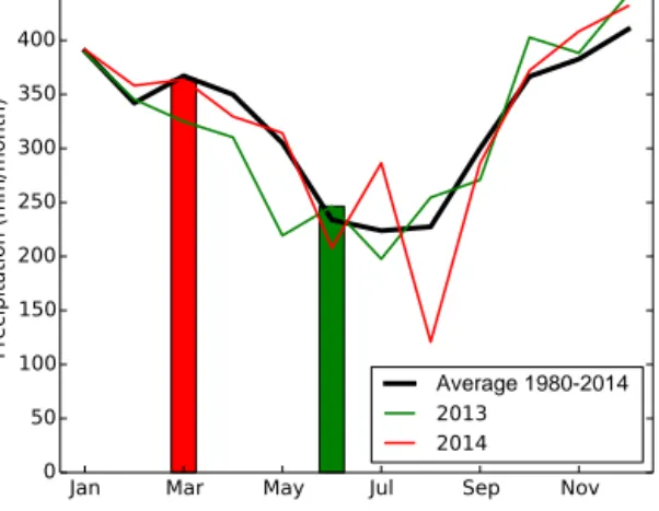
Figure 2. Average monthly precipitation during 1980–2014 (black), and monthly precipitation in 2013 (green) and 2014 (red). The bars indicate the rainfall during our sampling months. It can be seen that the rainfall pattern was not much different from the historical average during these periods.

3 Results 3.1 Discharge

Annual average precipitation from 1980 to 2014 amounted to 3903 mm yr⁻¹ in the chosen grid, corresponding to an average precipitation of 325 mm month⁻¹. The precipitation during June 2013 was below average (246 mm) and above average (364 mm) in March 2014. Both values do not de- viate much from the historical averages during 1980–2014 (March: 367 mm; June: 234 mm; see Fig. 2). In the following, we will refer to our measurements in June 2013 as representative of the dry season, and those in March 2014 as representative of the wet season.

With an average evapotranspiration of 4.2 mm d⁻¹ (Ku- magai et al., 2005), we estimated the average annual discharge for the Lupar river to be 490 and 160 m³s⁻¹ for the Saribas river. The flow velocities were estimated to be 2.5±1.4 m s⁻¹ (average±largest deviation from average) for the Lupar river, 0.7±0.7 m s⁻¹ for the Saribas, and 0.8±1.0 m s⁻¹for the Saribas tributary. Note that the measurements were taken during different stages of the tidal cycle, which explains the large variability.

3.2 Water chemistry

Our data covered a salinity range of 0–30.6 in the dry season and 0–31.0 in the wet season. Although relatively higher surface salinities were observed further upstream during the dry season if compared to the wet season, the geographical location of the mid-estuaries largely overlapped (Fig. 5a, b).

pH ranged between 6.7 and 8.0 in the dry season (2013) and between 6.8 and 7.6 in the wet season (2014) and was pos- itively correlated with surface salinity (r=0.8, data from both years). Notably, at salinity zero, pH was higher than

suggested by this correlation, and ranged between 6.7 and 7.3 (both seasons).

DIN concentrations in the surface water were generally rather low. During the dry season, DIN ranged between 1.7 and 87.1 µmol L⁻¹, whereas most concentrations were between 15 and 30 µmol L⁻¹. In the wet season, DIN concentrations ranged between 3.4 and 21.7 µmol L⁻¹. The medians for the individual estuaries show that overall, DIN concentrations were slightly higher in the dry season (Table 1).

Dissolved oxygen was mostly slightly undersaturated.

Oxygen saturation in the surface water was lower in the dry season than in the wet season (Table 1), with oxygen saturation ranging between 63.6–94.6 % (2013) and 79.0–100.4 % (2014). These values correspond to an AOU between 14 and 93 µmol L⁻¹(2013) and−1 and 52 µmol L⁻¹(2014), respectively. Negative AOU suggests net oxygen production and was only observed once in the lower estuary.

3.3 Organic carbon

DOC ranged from 80 to 784 µmol L⁻¹ in the dry season and from 172 to 1180 µmol L⁻¹in the wet season and was negatively correlated with salinity (Fig. 3), indicating that freshwater supplies DOC to the estuary, while seawater has a dilution effect. However, the end-member determined from the salinity-DOC correlation was not confirmed by the samples taken in the upper estuaries: the calculated end- member for Lupar was 673±274 µmol L⁻¹(intercept of the regression curve±standard error of the estimate), and the measured freshwater DOC median was 89 µmol L⁻¹(2013) and 208 µmol L⁻¹ (2014). For Saribas, the calculated end- member was 425±54 µmol L⁻¹, and the measured value was 312 µmol L⁻¹ (2013, Table 1). This discrepancy indicates that there is a source of DOC in the estuaries. With regards to their location, peatlands seemed a likely source of carbon to the estuaries. In a different study, we found DOC concentrations in a peat-draining river on the Maludam peninsula between 3612 and 3768 µmol L⁻¹(Müller et al., 2015).

With the average (3690 µmol L⁻¹) as a second zero-salinity end-member, we estimated how much carbon derives from peat-draining tributaries from the Maludam peninsula using a simple three-point mixing model (Fig. 3). The Maludam contributionf (in %) was calculated as

f = EM_calc− EM_meas

EM_Maludam− EM_meas·100, (6)

with EM_calc the calculated end-member, EM_meas the measured end-member and EM_Maludamthe peat-draining rivers’

end-member. Accordingly, 15 % of the DOC in the Lu- par river is derived from these peat-draining tributaries, and 3 % of DOC in the Saribas river. Following Baum et al.

(2007), the total DOC export to the ocean from Lupar and Saribas was estimated from the calculated zero-salinity end- members (673 and 425 µmol L⁻¹, respectively), assuming that they provide an average of non-peat and peat freshwa-

(6)

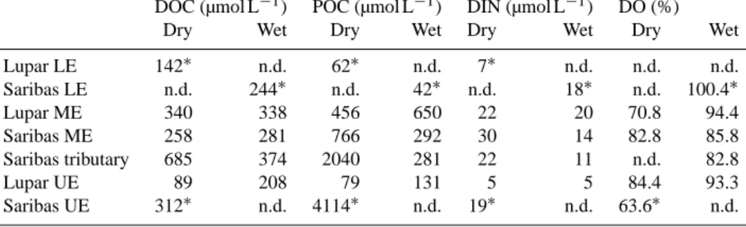
Table 1. Dissolved organic carbon (DOC), particulate organic carbon (POC) and dissolved inorganic nitrogen (DIN) median concentrations and oxygen saturation in the Lupar and Saribas estuaries.

DOC (µmol L⁻¹) POC (µmol L⁻¹) DIN (µmol L⁻¹) DO (%)

Dry Wet Dry Wet Dry Wet Dry Wet

Lupar LE 142^∗ n.d. 62^∗ n.d. 7^∗ n.d. n.d. n.d.

Saribas LE n.d. 244^∗ n.d. 42^∗ n.d. 18^∗ n.d. 100.4^∗

Lupar ME 340 338 456 650 22 20 70.8 94.4

Saribas ME 258 281 766 292 30 14 82.8 85.8

Saribas tributary 685 374 2040 281 22 11 n.d. 82.8

Lupar UE 89 208 79 131 5 5 84.4 93.3

Saribas UE 312^∗ n.d. 4114^∗ n.d. 19^∗ n.d. 63.6^∗ n.d.

LE: lower estuary (salinity>25). ME: mid-estuary (salinity 2–25, for the 2013 spatial extent of the rivers). UE: upper estuary.

∗denotes that only one data point was available.

0 5 10 15 20 25 30 Salinity 0

500 1000 1500 2000 2500 3000 3500

Doc (µmol L)−1

(a)

EMmeas

EMMaludam

EMcalc

Lupar

Dry (2013) Wet (2014)

0 5 10 15 20 25 30 Salinity

0 500 1000 1500 2000 2500 3000 3500

Doc (µmol L)−1

(b)

EMmeas

EMMaludam

EMcalc

Saribas

Dry (2013) Wet (2014)

Figure 3. Dissolved organic carbon (DOC) concentrations vs. salin- ity in the Lupar (a) and Saribas (b) estuaries. The red marker refers to the zero salinity end-member in the peat-draining tributaries. The line indicates the DOC-salinity regression line; labels refer to theo- retical and measured end-member values as described in the text.

ter inputs, and annual average discharge. Accordingly, Lupar and Saribas together convey 0.15±0.05 Tg yr⁻¹DOC to the South China Sea (Table 4).

Both the Lupar and Saribas estuaries were very turbid.

Suspended particulate matter (SPM) ranged from 3.7 to 5003.6 mg L⁻¹ in 2013 and from 13.8 to 3566.7 mg L⁻¹in 2014. Particulate organic carbon (POC) was higher during the dry season (Table 1), ranging from 51 to 4114 µmol L⁻¹ in 2013 and from 17 to 2907 µmol L⁻¹in 2014. The atomic carbon-to-nitrogen (C/N) ratio of particulate organic matter (POM) ranged between 8.5 and 14.1 in 2013 and between 8.1 and 13.8 in 2014 (see Fig. 4b).δ¹³C values ranged between−28.5 and−25.5 ‰ in 2013 and between−27.6 and

−24.4 ‰ in 2014. In contrast, the C/N ratio in the dissolved organic matter (DOM) was much higher: it ranged between 10.9 and 81.8 (2014 data; see Fig. 4a), whereas the lowest value was measured on the Lupar river, upstream of the Maludam peninsula, and the highest value was measured on the Lupar river at the mouth of a peat-draining left-bank tributary (see Fig. 1). The average for all samples was 40.6.

0 5 10 15 20 25 30 35 40 DON (µmol L⁻¹) 0

200 400 600 800 1000 1200

DOC (µmol L−1) peatleaves phytoplankton(a)

Lupar Saribas S.tributary

100 200 300 400 PON (µmol L⁻¹)

0500 10001500 20002500 30003500 4000

POC (µmol L−1) peat

leaves

phytoplankton (b)

Figure 4. Carbon-to-nitrogen (C/N) ratios in dissolved organic matter (a) and in particulate organic matter (b). Blue markers re- fer to samples from 2013; yellow markers refer to samples from 2014. The individual rivers are denoted by different symbols. Lines refer to the C/N ratios that would be expected for tropical peat and leaves (Baum, 2008) and for phytoplankton. Note that DON data shown in panel (a) were only available in 2014.

Since POC was not conservatively transported through the estuary, the export of POC to the South China Sea was estimated from the median POC concentration and discharge (see the Supplement). 0.10 Tg C yr⁻¹ are estimated to be delivered from the Lupar, and another 0.03 Tg C yr⁻¹ from the Saribas (Table 4). Taken together with the DOC export, this implies that Lupar and Saribas deliver approximately 0.3±0.2 Tg organic carbon to the South China Sea every year, approximately half of which is bound to particles.

3.4 CO₂and CO

In both years, both CO₂and CO were found to be above atmospheric equilibrium, indicating that the Lupar and Saribas estuaries were net sources of these gases to the atmosphere.

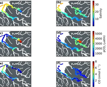
pCO₂ranged from 297 to 5504 µatm in 2013 and from 327 to 5014 µatm in 2014.pCO₂increased with decreasing salinity, indicating that highpCO₂can be attributed to freshwater input (Fig. 5). However, matters were different for the freshwater samples. The measured freshwater end-memberpCO₂

(7)

(a)

2013 (b) 2014

10 20 30

Salinity

(c) (d)

10002000 30004000 5000

pCO2 (µatm)

(e) (f)

2 4 6 8

CO (nmol L−1) Figure 5. Salinity (a, b), CO₂partial pressures (c, d) and CO con- centrations (e, f) measured during the two cruises in 2013 (left col- umn) and 2014 (right column).

was relatively moderate (1021–1527 µatm). Table 2 summa- rizes the medianpCO₂values in the lower, mid- and upper estuaries. It can be seen that like DOC,pCO₂was highest in the mid-estuaries. The difference between dry and wet season pCO₂was marginal (see Fig. 5). Excess CO₂(in µmol L⁻¹) was correlated with AOU for the Lupar river (dry season:

r=0.71,p=0.01; wet season:r=0.62,p=0.14). For the Saribas, the correlation was weak in the dry season (r=0.52, p=0.18). Due to the limited number of data points, no correlation could be established for the Saribas during the wet season (see Fig. 6).

Interestingly, Saribas and its tributary had a higherpCO2

(i.e., higherpCO2at the same salinity) than Lupar, but not higher DOC. δ¹³C-DIC ranged from−0.85 ‰ in the lower estuary to−15.70 ‰ in the freshwater region and increased with increasing salinity (not shown).

CO ranged from<0.1 to 5.8 nmol L⁻¹(<0.1 to 7.2 µatm) in the dry season (2013) and from 0.2 to 12.4 nmol L⁻¹(0.3 to 14.7 µatm) in the wet season (2014) and was spatially vari- able (Fig. 5). Median values are summarized in Table 2. CO concentrations were higher during daytime than during the night, independent of the boat’s location (Fig. 7). In both years, maximum CO concentrations were observed around noon and in the early afternoon. CO concentrations were not correlated with salinity, DOC, POC or SPM (not shown).

3.5 CO₂and CO fluxes

The CO₂ fluxes measured with the floating chamber showed large spatial variations and ranged from 63 to 935 mmol m⁻²d⁻¹. The lowest flux was measured in the Saribas mid-estuary, and the highest flux was measured on the Saribas tributary. k_600,FC values were averaged for the

20 0 20 40 60 80 100

AOU (µmol L⁻¹) 0

20 40 60 80 100 120 140

Excess CO (2µmol L)−1

1:1

Lupar, dry (2013) Saribas, dry (2013) Lupar, wet (2014)

Saribas, wet (2014) S.tributary, wet (2014)

Figure 6. Apparent oxygen utilization (AOU) vs. excess CO₂. Blue markers refer to samples from 2013; yellow markers refer to samples from 2014. The individual rivers are denoted by different symbols.

0 5 10 15 20

Hour of day LT 0

2 4 6 8 10 12 14

CO (n m ol L

−1

)

Dry (2013) Wet (2014)

Figure 7. CO concentrations depending on the hour of the day local time. The black areas refer to nighttime hours, while the light area denotes the daylight hours. All data are gathered in this figure; 2013 and 2014 data are distinguished with different colors and symbols.

Note that the boat was usually moving during daytime and more often not moving during nighttime.

individual rivers and are reported with the largest deviation of a single measurement from the mean. The Saribas tributary, which was the smallest of the studied rivers, had the highestk_600,FCof 23.9±14.8 cm h⁻¹. The largest river, Lu- par, had a highk_600,FCof 20.5±4.9 cm h⁻¹ as well, which is probably due to the high flow velocity (2.5 m s⁻¹). The Saribas main river had ak_600,FCof 13.2±11.0 cm h⁻¹, with

(8)

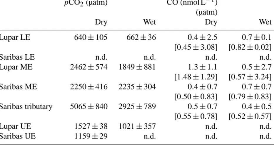
Table 2. Median CO₂partial pressures and CO concentrations (and partial pressures in brackets), respectively.

pCO₂(µatm) CO (nmol L⁻¹)

(µatm)

Dry Wet Dry Wet

Lupar LE 640±105 662±36 0.4±2.5 0.7±0.1

[0.45±3.08] [0.82±0.02]

Saribas LE n.d. n.d. n.d. n.d.

Lupar ME 2462±574 1849±881 1.3±1.1 0.5±2.7

[1.48±1.29] [0.57±3.24]

Saribas ME 2250±416 2235±304 0.4±0.7 0.7±0.7 [0.50±0.83] [0.79±0.83]

Saribas tributary 5065±840 2925±789 0.5±0.7 0.4±0.5 [0.55±0.78] [0.52±0.57]

Lupar UE 1527±38 1021±357 n.d. n.d.

Saribas UE 1159±29 n.d. n.d. n.d.

LE: lower estuary (salinity>25). ME: mid-estuary (salinity 2–25, for the 2013 spatial extent of the rivers). UE:

upper estuary. Values are median±1 standard deviation.

large spatial variability. The wind speed averaged 3.0 m s⁻¹ during our 2013 sampling period and 2.3 m s⁻¹ during the 2014 sampling period. The averagek_600,W92calculated with W92 were 1 order of magnitude lower than the experimen- tally determined ones, with 3.1 cm h⁻¹during the dry season and 1.9 cm h⁻¹during the wet season.

Atmospheric pCO₂ averaged 403.6 µatm in the dry season (2013) and 414.4 µatm in the wet season (2014). At- mospheric CO was 77.91 ppb in June 2013, corresponding to 77.49 natm. The average monthly mean for March was 145.93 ppb, corresponding to 145.58 natm. The calculated CO2and CO fluxes in the lower, mid- and upper estuaries are summarized in Table 3. Fluxes for the lower estuary were derived for the Lupar river (Fig. 5). Estimates for the upper estuaries were based on ourpCO₂measurements in the freshwater region and the averagek600,FCof Lupar and Saribas, respectively (Table 3). CO₂fluxes determined with the floating chamber (F_CO₂_,FC) ranged between 14 and 268 mol m⁻²yr⁻¹ and CO fluxes (F_CO,FC) between 0.7 and 1.8 mmol m⁻²yr⁻¹. For comparison, usingk_600,W92, we obtained CO₂fluxes between 2 and 30 mol m⁻²yr⁻¹.

Like pCO₂, the CO₂ fluxes were highest in the mid-estuaries, with F_CO₂_,FC ranging between 73 and 268 mol m⁻²yr⁻¹. The CO flux from Lupar was twice as high in the mid-estuary than in the lower estuary.

In order to calculate the total flux from these estuaries, we estimated the estuarine surface area of both systems in ArcGIS (for details see the Supplement). The Lupar estuary has a surface area of 220 km², which corresponds to 3 % of the catchment area, and the Saribas (excluding the tributary) estuary has a surface area of 102 km²(5 % of the catchment). The total water–atmosphere flux for the Lupar was 0.30±0.09 and 0.09±0.08 Tg C yr⁻¹ for the Saribas (see Table 4). The contribution of CO to these terms is negligi- ble.

4 Discussion

4.1 Sources and fate of carbon in the estuaries 4.1.1 Dissolved and particulate organic matter

It is striking that both DOC and CO2 are higher in the estuaries than in the freshwater region. This means that carbon is not conservatively transported to the ocean and that a source of both DOC and CO2exists in the estuaries. C/N ratios in DOM (average: 40.6) clearly suggest a terrestrial origin (Fig. 4a). Based on the calculated zero-salinity end- members, we estimated that 15 % of the DOC in the Lu- par and 3 % of the DOC in the Saribas estuary were derived from peat-draining tributaries. Given that peatlands cover 30.5 and 35.5 % of the catchments, we had expected a larger contribution. DOC concentrations in the Maludam river, the main river draining the Maludam peninsula, were more than ten times higher (3690 µmol L⁻¹, Müller et al., 2015) than the measured freshwater end-member of both Lu- par and Saribas. If we assume that all peat-draining tributaries exhibit these high DOC concentrations, elevated DOC concentrations would have been expected in the estuaries as well. Even though the estuarine DOC maximum indicates that peat-draining tributaries are indeed relevant sources of DOC to the estuaries, their contribution is small measured against the extent of peatlands in the catchment. Thus, the simple assumption that high-DOC inputs are proportional to the peatland coverage is not valid in this case, probably because the peatlands are located very close to the coast (Müller et al., 2015).

Likely, a part of the DOC that reaches the Lupar and Saribas estuaries is also retained through adsorption and floc- culation, which are promoted by mixing of saltwater and freshwater masses. Ertel et al. (1991) found that 1 to 12 % of DOC was converted to POC during laboratory experiments

(9)

Table 3. CO₂and CO fluxes in the Lupar and Saribas estuaries determined with a floating chamber.

FCO₂(mol m⁻²yr⁻¹) FCO (mmol m⁻¹yr⁻¹)

LE ME UE LE ME

Lupar 14±3 114±27 60±14 0.9±0.2 1.8±0.4

Saribas n.d. 73±61 33±28 n.d. 0.7±0.6

Saribas tributary n.d. 268±166 n.d. n.d. 0.9±0.6

LE: Lower estuariy (salinity>25). ME: Mid-estuary (salinity 2–25, for the 2013 spatial extent of the rivers). UE: upper estuary.

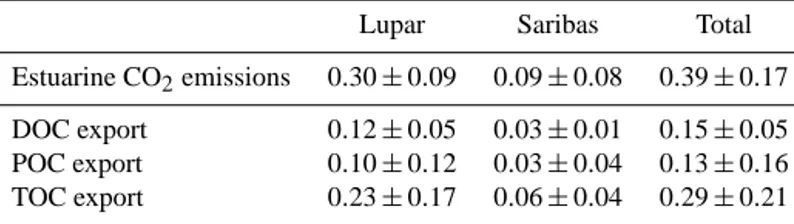
Table 4. Total carbon fluxes estimated for the Lupar and Saribas aquatic systems. All numbers are in Tg C yr⁻¹.

Lupar Saribas Total

Estuarine CO₂emissions 0.30±0.09 0.09±0.08 0.39±0.17 DOC export 0.12±0.05 0.03±0.01 0.15±0.05 POC export 0.10±0.12 0.03±0.04 0.13±0.16 TOC export 0.23±0.17 0.06±0.04 0.29±0.21

due to changes in salinity. The transformation of DOC to POC in the presence of saltwater was attributed both to particle precipitation and to adsorption of DOM onto riverine particles. Due to the high SPM concentrations in the Lupar and Saribas estuaries, we think that these processes could be important as well. A partial conversion of DOC to POC is consistent with the high POC concentrations and with the C/N ratios in particulate organic matter (POM) (8.1–14.1). This is likely a mixed signal from marine and terrestrial sources (Fig. 4b), in agreement with the relatively low δ¹³C values, which are indicative of both terrestrial soil and vascular plant material and phytoplankton (Bianchi and Bauer, 2011). We thus attribute those high POM concentrations to both river discharge and sediment resuspension due to the tidal currents.

In estuaries, POM may be degraded, deposited or exported to the continental shelf. It was shown that carbon burial in low-energy environments was a relevant sink of carbon in the Yangtze and Hudson estuaries (Zhu and Olsen, 2014).

For example, 42 % of the carbon deposited on intertidal sediments of the Scheldt estuary was buried (Middelburg et al., 1995), suggesting that sediments can make a significant contribution to the retention of carbon in estuaries. On the other hand, sediments can also act as a source of DOC to the estuarine waters, as DOC is released during the respiration of POC in sediments. This represents another possible explana- tion for the enhanced DOC levels in the estuaries if compared to the measured freshwater end-member.

4.1.2 Controls on CO₂

The elevatedpCO₂in the Lupar and Saribas estuaries and the depletion ofδ¹³C-DIC suggest that respiration plays an important role for the removal of organic matter (OM) in the

estuaries as well. Respiration could take place in the water column (pelagic respiration) or in the sediments (benthic respiration).

Generally, pelagic respiration rates are largely controlled by temperature and the availability of organic substrates (Hopkinson Jr. and Smith, 2005). The relatively high concentrations of terrestrial organic matter (DOM + POM) and the high temperatures in the Lupar and Saribas estuaries suggest considerable rates of pelagic respiration, which would explain the relatively highpCO₂and the correlation of CO₂ and AOU. The fact that this correlation was weak can be explained by the presence of other controls on CO₂(pH, trans- port) as well as the buffering capacity of the carbonate system, whereas changes in CO₂are buffered by DIC.

EstuarinepCO₂is usually highest in high-turbidity zones (Abril and Borges, 2004), where the light penetration depth and thereby photosynthetic CO2 uptake are limited. At the same time, the residence time of organic matter is prolonged (Abril et al., 1999), and particle-attached bacteria get the chance to decompose OM (Crump et al., 1998), resulting in pronounced net heterotrophy. Due to the strong tidal currents in the Lupar and Saribas estuaries, particle sedimentation is probably delayed by turbulence, leaving more time for the pelagic community to respire OM (Hopkinson Jr. and Smith, 2005).

Benthic respiration accounts on average for 24 % of the total system production in estuaries (Hopkinson Jr. and Smith, 2005). Although this respiration is largely aerobic, OM decomposition can also occur through denitrification, man- ganese, iron or sulfate reduction and methanogenesis. Mid- delburg et al. (1995) showed that 58 % of the carbon delivered to intertidal sediments in the Scheldt estuary was rem- ineralized. The produced CO2may be detected in estuarine waters (Cai et al., 1999) or escape to the atmosphere from

(10)

the exposed sediment surface. This represents an additional CO₂flux that we did not account for in our study. Therefore, future work should include the carbon supply to and reminer- alization rates in intertidal sediments.

Although pCO₂ is relatively high, oxygen depletion is quite moderate in comparison. For example, Chen et al.

(2008) measured CO₂ partial pressures between 690 and 2680 µatm in the eutrophicated Pearl river estuary (see Ta- ble 5) along with AOU up to 239 µmol kg⁻¹, resulting in hy- poxia at the river mouth. Although we found similarly high and even higherpCO2, oxygen depletion was much less pronounced. This suggests that more oxygen is available in the Lupar and Saribas estuaries. Reaeration might be more efficient, i.e., oxygen fluxes across the air–water interface are higher, which could be explained by a high gas exchange velocity, consistent with our measurements, and a shallower water column.

Another important control on pCO₂ is pH, which var- ied spatially by 1.3 (2013) and 0.8 (2014) in the Lupar and Saribas estuaries. This can largely be attributed to the mixing of seawater and freshwater along the estuary, as indicated by the correlation of pH with salinity. Additionally, inputs from peat-draining rivers, which are highly acidic (pH<4, Kselik and Liong, 2004; Müller et al., 2015), might decrease pH. Lower pH shifts the carbonate system towards more free CO2, consistent with the elevatedpCO2observed in the Lu- par and Saribas estuaries. On the other hand, respiratory CO2

might decrease pH. It cannot be ultimately resolved whether the pH drives pCO2 or whether respiration drives the pH.

In situ measurements of pelagic and benthic respiration rates could help resolve details about these mechanisms.

4.1.3 Photochemical degradation of organic matter In addition to respiration, the diurnal CO cycle observed in the Lupar and Saribas estuaries (Fig. 7) suggests that photodegradation is another pathway for the removal of DOC.

This diurnal pattern is well known for ocean surface water and explained by a balance of light-dependent production of CO and microbial consumption (Conrad and Seiler, 1980;

Conrad et al., 1982; Ohta, 1997). Average CO concentrations in the Lupar and Saribas estuaries were lower than in the East China Sea and Yellow Sea (average 2.25 nmol L⁻¹, Yang et al. (2011); see Table 5), which can be attributed to the high turbidity. A high concentration of suspended particulates limits the light penetration depth and increases microbial CO consumption (Law et al., 2002). On the other hand, CO can also be photochemically produced from particles (Xie and Zafiriou, 2009). These authors found that in coastal waters, CO photoproduction from particulates was 10–35 % that of CDOM. We could not establish a clear relationship between SPM and CO for the Lupar and Saribas estuaries.

However, the low CO concentrations suggest that particulates limited CO photoproduction rather than supported it.

Another reason for the low CO concentrations could be that

the terrestrial DOM in the Lupar and Saribas estuaries is not so susceptible to photodegradation, which would be in contrast to other studies (Valentine and Zepp, 1993; Zhang et al., 2006).

However, it would be too fast to conclude that photochemistry is only of little relevance for the DOM removal in our study area. First of all, most CO is probably produced di- rectly at the water surface and might quickly escape to the atmosphere. We might not have captured this volatile CO fraction with our measurements, since we sampled water from 1 m below the surface. While CDOM absorption is highest in the UV (e.g., Kitidis et al., 2011), the attenuation of light in natural waters is strongest in the UV as well. Therefore, CO concentrations usually decline rapidly with water depth (Ohta et al., 2000), so the numbers presented here can be considered conservative. Secondly, the relevance of photochemistry amounts to more than CO production. UV radia- tion changes the composition of CDOM (Zhang et al., 2009), which changes its bioavailability (Amon and Benner, 1996;

Moran et al., 2000). Tranvik et al. (2000) showed that in nutrient-poor (oligotrophic) systems, the net effect of radi- ation is an enhancement of bacterial growth, as photochemical reactions increased not only the bioavailability of organic carbon compounds, but also of nitrogen and phosphorous.

However, other studies have shown that photochemical reactions consume molecular oxygen (Kitidis et al., 2014) and produce reactive oxygen species (ROS), which may decrease the bioavailability of DOM (Scully et al., 2003). Thus, the role of photochemistry in our study area beyond the mere production of CO remains uncertain and would merit further investigation.

4.2 Comparison dry season vs. wet season

Expectedly, the differences between dry season and wet season DOC were marginal, which is in agreement with other studies in this region. Moore et al. (2011) argued that DOC concentrations vary only little, because DOC is released to rivers throughout the year due to the high precipitation. They found that POC concentrations exhibited a clear seasonal- ity, with higher concentrations during the dry season. Consis- tently, this was also observed in our study. The higher AOU and DIN values in the dry season indicate that respiration was higher then, possibly due to enhanced respiration of POC.

The higher availability of POC in the dry season was most obvious in the Saribas and its tributary, whereas in the latter, the hypothesis of POC-enhanced respiration is confirmed by slightly higherpCO₂. For Lupar and the Saribas main river, though, we did not observe any major differences between wet and dry seasonpCO₂and CO concentrations. The weak seasonal variability has some general implications for the research in our study area, which is mostly based on single campaigns and not on continuous measurements due to poor infrastructure. The little variation that we observe between our wet and dry season measurements could imply that sin-

(11)

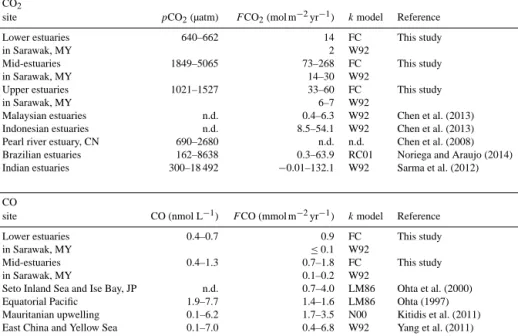
Table 5. Comparison of CO₂and CO values for partial pressure and concentration, respectively, and fluxes for different tropical and subtropical sites.

CO₂

site pCO₂(µatm) FCO₂(mol m⁻²yr⁻¹) kmodel Reference

Lower estuaries 640–662 14 FC This study

in Sarawak, MY 2 W92

Mid-estuaries 1849–5065 73–268 FC This study

in Sarawak, MY 14–30 W92

Upper estuaries 1021–1527 33–60 FC This study

in Sarawak, MY 6–7 W92

Malaysian estuaries n.d. 0.4–6.3 W92 Chen et al. (2013)

Indonesian estuaries n.d. 8.5–54.1 W92 Chen et al. (2013)

Pearl river estuary, CN 690–2680 n.d. n.d. Chen et al. (2008)

Brazilian estuaries 162–8638 0.3–63.9 RC01 Noriega and Araujo (2014)

Indian estuaries 300–18 492 −0.01–132.1 W92 Sarma et al. (2012)

CO

site CO (nmol L⁻¹) FCO (mmol m⁻²yr⁻¹) kmodel Reference

Lower estuaries 0.4–0.7 0.9 FC This study

in Sarawak, MY ≤0.1 W92

Mid-estuaries 0.4–1.3 0.7–1.8 FC This study

in Sarawak, MY 0.1–0.2 W92

Seto Inland Sea and Ise Bay, JP n.d. 0.7–4.0 LM86 Ohta et al. (2000)

Equatorial Pacific 1.9–7.7 1.4–1.6 LM86 Ohta (1997)

Mauritanian upwelling 0.1–6.2 1.7–3.5 N00 Kitidis et al. (2011)

East China and Yellow Sea 0.1–7.0 0.4–6.8 W92 Yang et al. (2011)

The gas exchange velocitykused to calculate the flux was determined using different approaches: FC=floating chamber measurements. W92=Wanninkhof (1992). N00=Nightingale et al. (2000). LM86=Liss and Merlivat (1986). RC01=Raymond and Cole (2001).

gle measurement campaigns in this region provide better in- sights than previously assumed. However, measurements at the peak of the monsoon season would be desirable to confirm this hypothesis.

4.3 CO₂and CO fluxes

It has been previously suggested that Southeast Asian estuaries are rather moderate sources of CO₂to the atmosphere, because of low wind speeds and consequently low transfer velocities (Chen et al., 2013). We cannot confirm this no- tion with our measurements. CO₂ emissions from both the Lupar mid-estuary (F_CO₂_,FC = 114±27 mol m⁻²yr⁻¹) and the Saribas tributary (F_CO₂_,FC = 268±166 mol m⁻²yr⁻¹) are higher than the global average of 37.4 mol m⁻²yr⁻¹ for mid-estuaries (Chen et al., 2012). Certainly, elevated CO2fluxes can be partially attributed to high temperatures, which decrease the solubility of CO2in water and increase the gas exchange velocity. However, the average value reported for small deltas in this region is 41.8 mol m⁻²yr⁻¹ (Laruelle et al., 2013), which is also lower than the fluxes from Lupar and the Saribas tributary. The fluxes from the Saribas mid-estuary appear to be higher than those values, too (F_CO₂_,FC=73±61 mol m⁻²yr⁻¹), but we cannot ascer- tain this because of the large uncertainty range. Interestingly, the fluxes that we found are also more than 1 order of magnitude higher than areal fluxes reported for Indian monsoonal estuaries (Sarma et al., 2012) and for other Malaysian rivers (Chen et al., 2013); see Table 5. However, flux estimates depend critically on the gas exchange velocity: both Sarma

et al. (2012) and Chen et al. (2013) used the W92 parameterization for calculating the gas exchange velocity. The comparison between FCO₂,FC andFCO₂,W92 revealed a considerable difference (see Table 5). However,F_CO₂_,W92 in the mid-estuaries was still higher (14–30 mol m⁻²yr⁻¹) than the values of Chen et al. (2013), and could indicate that the presence of peatlands makes a notable difference for CO₂emissions from tropical estuaries.

CO flux estimates (F_CO,FC) were in a similar range as those obtained for the Mauritanian upwelling (Kitidis et al., 2011), and those reported for the equatorial Pacific upwelling (Ohta, 1997) and for the East China Sea and Yellow Sea (Yang et al., 2011) (see Table 5). However, if we useFCO,W92

for comparison, it seems that CO fluxes are rather low in our study area, consistent with the observation that CO concentrations appear to be rather low, as discussed above.

Both the CO₂ flux estimates and the CO flux estimates presented in this study and elsewhere depend critically on the gas exchange velocity. The W92 exchange velocities dif- fered considerably from our experimental values, yielding much lower fluxes. We believe that the W92 parameterization, which was derived for the ocean, is not suitable for estuaries, though frequently used. It does not account for the turbulence created by tidal currents and water flow velocity. Borges et al. (2004) showed that the contribution of the water-current related gas exchange velocity to the total gas exchange velocity was substantial at low wind speeds, which are prevalent in our case, too. Therefore, we think that it is more accurate to use empirically determined exchange velocities over wind speed parameterizations.

(12)

The performance of floating chambers has been a matter of debate. Arguments exist both for floating chambers leading to overestimation and underestimation of the flux: because they shield the water surface from wind, they may re- duce the gas exchange (Frankignoulle, 1988). However, in our case, k_600,FC were much higher than k_600,W92, so that here, the question is rather whether the floating chamber method leads to an overestimation of the flux. This would have been the case if the chamber had created artificial tur- bulences. Indeed, this has been discussed as one of the major weaknesses of the floating chamber method (Matthews et al., 2003; Vachon et al., 2010), although chambers are more susceptible to disruptions in low-turbulence environments than in high-turbulence environments (Vachon et al., 2010). In contrast, a recent study found a rather good agreement between floating chamber and eddy covariance measurements on a river (Huotari et al., 2013), which suggests that the accuracy of floating chamber measurements is also a matter of de- sign. We intended to avoid creation of artificial turbulence by (1) using short wall extensions of the chamber into the water (ca. 1 cm), which is thought to decrease the artificial turbulence by making the chamber more stable (Matthews et al., 2003), and (2) letting the chamber float freely next to the boat. Our setup could be improved by monitoring the temperature in the chamber headspace, which was not done during this study. We assumed that the temperature increase was limited because of the short time of deployment (5–10 min).

Taken together, Lupar and Saribas deliver 0.3 Tg organic carbon to the South China Sea every year and release 0.4 TgC to the atmosphere as CO2.

5 Conclusions

Overall, we conclude that these estuaries in a peat-dominated region receive considerable amounts of terrestrial organic carbon, only a minor part of which was contributed by peat- draining tributaries, however. Estuarine pCO₂ was largely driven by aerobic respiration of OM and pH variability. OM degradation was likely supported by photochemistry, as indicated by a diurnal variability of CO concentrations in the surface water. Overall, CO2emissions to the atmosphere were substantial if compared to other tropical and subtropical sites, while CO emissions were moderate, because photoproduction was limited by a high turbidity. We suggested that the use of a wind-driven turbulent diffusivity model (W92) leads to a gross underestimation of the fluxes, because it neglects turbulence caused by tidal currents and river discharge. Aside from net heterotrophy, we hypothesized that a fraction of the DOC was removed by adsorption onto estuarine particles. This highlights how these estuaries function as an efficient filter between land and ocean. Unlike small peat-draining rivers, which tend to export most organic carbon downstream, the adjacent estuaries seem to trap a large fraction of this terrestrial organic carbon. This means that the carbon export to the

continental shelf is reduced, at the price of CO₂production and, ultimately, emission from the estuary.

The Supplement related to this article is available online at doi:10.5194/bg-13-691-2016-supplement.

Acknowledgements. We would like to thank the Sarawak Bio- diversity Center for permission to conduct research in Sarawak waters (permit no. SBC-RA-0097-MM and export permit SBC-EP- 0040-MM). We thank Hella van Asperen (University of Bremen, Germany), Nastassia Denis, Felicity Kuek, Joanne Yeo, Hong Chang Lim, Edwin Sia (all Swinburne University, Malaysia) and all scientists and students from Swinburne University and the University of Malaysia Sarawak who were involved in the sampling campaigns and the preparation. Lukas Chin and the crew members of the SeaWonder are acknowledged for their extensive support.

We would also like to acknowledge Innovasi Samudra Sdn Bhd for the loan of the CTD equipment. The authors thank Matthias Birkicht and Dorothee Dasbach (ZMT Bremen, Germany) for their help in the lab performing the analyses. Ultimately, we acknowledge the University of Bremen for funding this study through the “exploratory project” in the framework of the University’s Institutional Strategy. The development of the FTIR measurements was supported by EU FP7 project InGOS. The authors thank three anonymous referees for their comments and suggestions which significantly improved the manuscript.

The article processing charges for this open-access publication were covered by the University of Bremen.

Edited by: M. Dai

References

Abril, G. and Borges, A. V.: Carbon Dioxide and Methane Emis- sions from Estuaries, in: Greenhouse Gas Emissions: Fluxes and Processes, Hydroelectric Reservoirs and Natural Environ- ments, Environmental Science Series, Springer, Berlin, Heidel- berg, New York, chapt. 7, 187–207, 2004.

Abril, G., Etcheber, H., Hir, P. L., Bassoullet, P., Boutier, B., and Frankignoulle, M.: Oxic/anoxic oscillations and organic carbon mineralization in an estuarine maximum turbidity zone (the Gironde, France), Limnol. Oceanogr., 44, 1304–1315, 1999.

Alkhatib, M., Jennerjahn, T. C., and Samiaji, J.: Biogeochemistry of the Dumai River Estuary, Sumatra, Indonesia, a tropical black- water river, Limnol. Oceanogr., 52, 2410–2417, 2007.

Amon, R. M. W. and Benner, R.: Photochemical and microbial consumption of dissolved organic carbon and dissolved oxygen in the Amazon River system, Geochim. Cosmochim. Ac., 60, 1783–

1792, 1996.

Andriesse, J. P.: Nature and Manamanage of Tropical Peat Soils, FAO Soils Bulletin 59, Food and Agriculture Organization of the United Nations (FAO), Rome, 1988.

Fate of terrestrial organic carbon and associated CO2