Research Collection
Working Paper
Synthesising digital twin travellers
Individual travel demand from aggregated mobile phone data
Author(s):
Anda, Cuauhtémoc; Ordonez Medina, Sergio Arturo; Axhausen, Kay W.
Publication Date:
2020-09
Permanent Link:
https://doi.org/10.3929/ethz-b-000442517
Rights / License:
In Copyright - Non-Commercial Use Permitted
This page was generated automatically upon download from the ETH Zurich Research Collection. For more information please consult the Terms of use.
ETH Library
Synthesising Digital Twin Travellers: Individual travel demand from aggregated mobile phone data
Cuauhtemoc Andaa,∗, Sergio A. Ordonez Medinaa, Kay W. Axhausenb
aFuture Cities Laboratory, ETH Zurich, 1 Create Way #06-01, Singapore 138602
bIVT, ETH, Wolfgang-Pauli-Strasse 15, HIL F31.1, 8093 Zurich, Switzerland
Abstract
Mobile phone data generated in mobile communication networks has the potential to improve cur- rent travel demand models and in general, how we plan for better urban transportation systems.
However, due to its high-dimensionality, even if anonymised there still exists the possibility to re- identify the users behind the mobile phone traces. This risk makes its usage outside the telecom- munication network incompatible with recent data privacy regulations, hampering its adoption in transportation-related applications. To address this issue, we propose a framework designed only with user-aggregated mobile phone data to synthesise realistic daily individual mobility — Digi- tal Twin Travellers. We explore different strategies built around modified Markov models and an adaption of the Rejection Sampling algorithm to recreate realistic daily schedules and locations.
We also define a one-day mobility population score to measure the similarity between the popula- tion of generated agents and the real mobile phone user population. Ultimately, we show how with a series of histograms provided by the telecommunication service provider (TSP) it is possible and plausible to disaggregate them into new synthetic and useful individual-level information, building in this way a big data travel demand framework that is designed in accordance with current data privacy regulations.
Keywords: travel demand models, mobile phone data, generative models, data privacy
1. Introduction
1
New streams of geo-codedBig Dataallows us to observe and understand mobility behaviour on
2
an unprecedented level of detail (Anda et al., 2017). From this array of data sources, mobile phone
3
network data from the telecommunications service providers (TSP) has drawn special attention
4
in the transportation field due to its pervasiveness, extensive coverage, and persistent collection.
5
These records are generated in the telecommunications network as a result of user-related events
6
such as voice calls and internet usage, and network-related events such as location area changes
7
and periodical network updates. Once an event is triggered, a timestamp and the mobile device
8
id are recorded in a cell tower, normally the closest to the mobile device. In such way that if the
9
∗Corresponding author.
Email address:anda@arch.ethz.ch(Cuauhtemoc Anda)
timestamps were filtered by mobile id, sorted by time of the day and plotted on a map, we would
10
obtain a view of visited locations and trajectories of a mobile phone user. This enables a wide
11
range of research towards using mobile phone data to improve travel demand models (Iqbal et al.,
12
2014; Alexander et al., 2015; Toole et al., 2015; Molloy and Moeckel, 2017; Bwambale et al.,
13
2019) and uncover insights into human mobility (Gonzalez et al., 2008; Song et al., 2010).
14
Conversely, the fact that individual daily mobility patterns can be reconstructed from a series
15
of mobile phone data points has awakened growing concerns in regards to data privacy (Valentino-
16
DeVries et al., 2018). People’s patterns of movement in space and time are highly dimensional,
17
making mobile phone data a potent quasi-identifier for a single person (International Transport
18
Forum, 2015). For instance, De Montjoye et al. (2013) found that even for data with a temporal
19
resolution of an hour and a spatial resolution equal to the density of cell towers, just four spatio-
20
temporal points were sufficient to isolate and uniquely identify 95% of the individuals.
21
The emergence ofBig Datahas pushed forward recent updates on data protection and privacy
22
regulations. New provisions and requirements that extend the responsibilities related to personal
23
data processing have been included in different regulations. For example, recital 26 of the Euro-
24
pean General Data Protection Regulation (GDPR) (European Commission, 2018) states that the
25
principles of data protection should apply to any information concerning an identified or identifi-
26
able natural person or to personal data which have undergonepseudonymisationwhich could be
27
attributed to a natural person by using additional information. This means that ’anonymising’ mo-
28
bile phone network data sets is not enough to comply with the GDPR (similarly with other privacy
29
regulations like the Singapore Personal Data Protection Act (PDPA) (Personal Data Protection
30
Commission Singapore, 2012)). The result is an additional barrier-to-adopting mobile phone data
31
into transport planning since it becomes a challenge to strike a balance between data privacy and
32
data utility.
33
One possibility to comply with these regulations is to group data in such a way that individual
34
records no longer exist and cannot be distinguished from other records in the same grouping. In
35
this scenario, we are only able to request user-aggregated histograms from the TSPs. Therefore,
36
what we present here are some ideas on how mobile phone data utility can be maximised under
37
this circumstance. With the premise of disaggregating aggregated data into an alternative but rep-
38
resentative mobility population, we have developed a framework built around modified Markov
39
models and an adaption of the rejection sampling algorithm to produce realistic synthetic individ-
40
ual level mobility data at an urban scale. The output of this work can be used, for example, to set
41
up agent-based transport simulations (Anda et al., 2018; Bassolas et al., 2019).
42
The remainder of this paper is organised as follows. In Section 2, we review the related work on
43
travel demand and generative models. Section 3 provides an overview of the general framework.
44
In Section 4, we introduce the modified Markov models along with a baseline Markov model.
45
Section 5 shows the clustering strategy used to segment mobile phone users. Section 6 explains
46
how the models and strategies were evaluated and shows the results obtained. Finally, Section 7
47
and 8 contain further discussion and the conclusions, respectively.
48
2. Literature Review
49
The traditional approach to model travel demand is by means of the four-step travel model
50
(de Dios Ort´uzar and Willumsen, 2011). It is comprised by a trip generation step, where land-use
51
related factors are employed to calculate the incoming and outgoing number of trips per aggregate
52
zone level; trip distribution, which allocates those trips into origin-destination pairs following a
53
gravity model function; mode choice, to compute the proportion of trips by transportation mode,
54
generally by using a utility-maximisation choice model; and traffic assignment, which allocates the
55
routes taken following the Wardrop’s principle of user-equilibrium. The final output is an estimate
56
of travel demand aggregated at the zone level.
57
In recent years, a new transport forecasting approach has emerged based on agent-based sim-
58
ulations. Where instead of focusing on zones, the main axis of the analysis is the individuals and
59
their travel and activity plans (Axhausen and G¨arling, 1992). For this disaggregated paradigm,
60
travel demand models have been developed accordingly. Prominent examples are Bowman and
61
Ben-Akiva (2001), where individual tours with activities and itineraries are constructed through a
62
series of discrete choice models; and Arentze and Timmermans (2000), where the choice of dif-
63
ferent daily plan aspects are modelled through a series of decision trees. In both cases the models
64
are developed around household travel surveys, which include socio-demographic information.
65
Mobile phone data is a natural fit into the disaggregated modelling paradigm, however, seldom
66
times one has access to socio-demographic information which is required in travel survey-centric
67
travel demand models. In addition, mobile phone data embeds other type of characteristics that
68
can potentially improve the current transport planning capabilities. This has called for the devel-
69
opment of new mobile phone data-tailored travel demand models. Jiang et al. (2016) proposed
70
TimeGeo, a travel demand framework without travel surveys. InTimeGeo, home and work activity
71
locations are inferred from mobile phone data first, then locations and schedules of flexible (i.e.
72
secondary) activities are simulated using spatial and temporal mechanisms of human dynamics.
73
Lin et al. (2017) similarly inferred primary activity locations from mobile phone data, but trained
74
instead a Long Short Term Memory (LSTM) Recurrent Neural Network (RNN) to model flexible
75
activities. In both studies, access to individual-level mobile phone data was required, as well as
76
the identification of home and work locations of mobile phone users. This can become problem-
77
atic when transferred into practice, specifically in cases where stakeholders are required to comply
78
with data privacy regulations.
79
A possible solution to the privacy problem is to use synthetic data as an alternative to real
80
users’ data. This idea has emerged in the computer science domain as part of a line of research
81
that focuses on different methods to ensure data privacy in user trajectory data. There are several
82
notable examples with similar objectives to this work but with important differences. Isaacman
83
et al. (2012) introduced WHERE, a probabilistic modelling approach to produce synthetic Call
84
Detail Records (CDRs). Later, Mir et al. (2013) extended the approach to add a differential privacy
85
mechanism (DP-WHERE) as a formal privacy-preservation guarantee. For both cases, synthetic
86
CDRs are generated from a series of distributions related to home/work locations and call patterns.
87
One of the key differences with this study is that in mobile phone network data full location
88
trajectories can be usually derived, whereas, in CDRs the location is only known at the time when
89
a call is made. Hence, this paper can be considered an updated version of Isaacman et al. (2012).
90
Another relevant example is the work by Bindschaedler and Shokri (2016). Here, a Markov
91
model is trained on a set of seed traces to synthesise plausible location traces. The model incor-
92
porates current location (i.e. the state) and a period of time random variable (morning, afternoon,
93
evening and night) to predict/generate the next location following a semantic seed structure. Addi-
94
tionally, geographic and semantic similarity metrics were also defined to evaluate the performance
95
of the synthetic traces. It is important to note that this framework was designed to generate re-
96
alistic but independent location traces, thus, no guarantees or validation exist for a population of
97
urban-wide mobility traces. Moreover, given how individual traces are sampled from seeds (i.e.
98
adding noise to the Viterbi reconstruction step), if a population of traces were generated, it would
99
most probably lose the statistical properties of the real population.
100
More recently, the work by Pappalardo and Simini (2018) looked into generating samples of
101
realistic spatio-temporal trajectories while remaining as close as possible to several real population
102
statistics. They proposed a two-step framework. First, a Markov chain (non-parametric) to trans-
103
form a base diary with only home locations into a mobility diary containing additional abstract
104
locations. Second, the use of an exploration and preferential return (parametric) model to allocate
105
the geographical information of the abstract locations. Although the framework outputs individual
106
mobility trajectories, as mentioned by the authors, these mobility trajectories exclude travel times.
107
Furthermore, their validation excludes relevant aspects in transportation, like the distribution of
108
tours/mobility motifs Schneider et al. (2013), making the accuracy of their results uncertain for
109
transport-specific applications.
110
From the literature, it emerges the importance to continue developing new urban-scale travel
111
demand models based on mobile phone network data. In particular, models that are capable of
112
generating realistic and individual mobility trajectories, including locations, activity/stay times
113
and durations, and travel times. All of these, while considering the implications and considera-
114
tions of deploying them into real-world transport-specific applications. Namely, transport-oriented
115
validation results that confirm the data-utility for applications in this field, and the data-sharing
116
constraints between practitioners and TSPs due to data privacy regulations.
117
Position of our work. As an effort to close the research gap towards the aforementioned direction,
118
in this paper, we introduce the Digital Twin Travellers framework to synthesise individual travel
119
demand from aggregated mobile phone data. Different to Isaacman et al. (2012) and Mir et al.
120
(2013), our proposed framework is based on trajectories derived from mobile phone data where
121
location updates are not exclusive to calls (i.e. CDRs) but also come from other user-intrinsic
122
events (e.g. internet usage) as well as other user-extrinsic mechanisms (e.g. transition between
123
cell-location areas). Also, as opposed to Jiang et al. (2016) and Pappalardo and Simini (2018),
124
our approach is a fully data-driven non-parametric model that does not require the inference of
125
home and work locations. It is also an integrated generative framework, meaning that the spatial
126
and temporal components are not split (Pappalardo and Simini, 2018), and where the objective is
127
to estimate a joint probability distribution of mobility patterns in a population. This allows, for
128
instance, to recreate the number of trips per agent as part of the Markov process rather than from a
129
predefined base itinerary or seed (Bindschaedler and Shokri, 2016; Pappalardo and Simini, 2018).
130
It also ensures the statistical match among several distributions directly modelled. Finally, another
131
important difference is the restriction of user-aggregated data as input. This is to align the frame-
132
work to recent data privacy regulations and make it readily-available for real-world applications.
133
Another benefit of relying uniquely on aggregated data is that the proposed framework serves as
134
the foundation for a future iteration where formal privacy-guarantees can be added, similar to Mir
135
et al. (2013). Bindschaedler and Shokri (2016) noted the drawbacks on using only aggregates of
136
data to synthesise new mobility traces, in particular the result of unlikely traces that do not adhere
137
to realistic mobility constraints. In this work, we explore different strategies in the generative mod-
138
elling framework and sampling methods to compensate for this. These strategies aim to maximise
139
data accuracy for transport applications while keeping efficient model designs with generalisation
140
capabilities. It is also important to mention that generative modelling techniques have already
141
being explored in the field of transportation, principally to produce synthetic populations (Sun
142
and Erath, 2015) (Sun et al., 2018) (Borysov et al., 2019), simulate activity chains (Axhausen and
143
Herz, 1989), and generate mobility patterns (Lin et al., 2017) (Ouyang et al., 2018).
144
Thus, the contribution of this work is threefold. First, we propose the non-parametric and fully
145
data-driven Digital Twin Travellers framework to synthesise realistic spatio-temporal trajectories
146
from aggregated mobile phone data. Second, we define a validation metric to compare synthetic
147
populations of disaggregated mobility data with real ones, the one-day mobility population accu-
148
racy score, which is oriented to transportation-specific applications and which considers relevant
149
distributions often not validated, such as the distribution of tours. Third, the exploration between
150
model complexity and accuracy between different strategies within a generative modelling frame-
151
work to synthesise realistic spatio-temporal trajectories. All of these, with the ultimate objective of
152
enabling the usage of mobile phone data in disaggregated transport applications (e.g. agent-based
153
simulations) while complying with recent data privacy regulations.
154
3. General Framework
155
The objective is to synthesise realistic and individual daily travel demand in the form of stay-
156
point trajectories, or as defined by Pappalardo and Simini (2018), mobility diaries containing the
157
time and duration of the visits in the various locations without explicitly specifying the type of
158
activity. More specifically, we define a stay-point as a location (i.e. the stay-zone) where a user
159
remains for at least 15 minutes, along with its start time and end time. In terms of the four step
160
model, the proposed work solves the trip generation and trip distribution steps in a disaggregated
161
manner. All these under the premise that we have access to mobile phone data representative of the
162
population, but this access is restricted to only user-aggregated queries. Hence, the output could
163
be used to:
164
1. Generate the complementary individual travel demand data of users subscribed to a different
165
TSP.
166
2. Generate a full digital twin population with complete one-day tours (i.e. Digital Twin Trav-
167
ellers).
168
We start by assuming that there exists a true distribution that describes the mobility patterns of
169
an entire urban population. This true distribution (eq. 1) encodes the joint probability distribution
170
of the sequence of stay-points visited by an individual during one day.
171
fX(x)= P(X1 =x1,X2 =x2, ...,XN =xN) (1) On eq. 1, eachXicorresponds to a set of random variables that describe the spatial and tempo-
172
ral aspects of theithstay-point. For example,Xican be the tuple of random variables [Zi,S ti,Di]:
173
the ith stay-zone, start time and duration respectively. xi is the set of realisations of the random
174
variables inXi. Each individual has a total ofN stay locations throughout a day.
175
The main strategy is to approach as much as possible to this true distribution by constructing
176
a proposal distribution gX(x) that encloses the real distribution fX(x). Then, follow up with an
177
adaptation of the rejection sampling algorithm to improve over the model deficiencies and ulti-
178
mately get individual mobility demand samples that have similar statistics as the ones in the real
179
population.
180
3.1. Markov Models
181
Given the complexity in eq. 1, we require a modelling framework that is computationally
182
feasible and simplifies the joint distribution by factorising it into a set of marginal and conditional
183
probability distributions. We employ Dynamic Bayesian Networks to build different Markov mod-
184
els that can approximate fX(x). These type of models are commonly used to describe the different
185
states in a dynamical system. We interpret individual travel demand as a dynamical system, where
186
the different stay-zones represent the different states of the individual. The essence of Markov
187
models is that the immediate future state of a system depends only in the current state, thus, dis-
188
regarding any information on previous states, this is called the first-order Markov property. For
189
our case of interest, the first-order Markov property represents an important constraint if we de-
190
sire to model realistic daily tours. We represent daily tours as mobility networks derived from
191
the stay-zones visited by an individual on a single day. Each node in the network represents a
192
different stay-zone, and the links indicate the trips done between stay-zones. This is similar to the
193
definition ofmobility motifsin Schneider et al. (2013). As an example, if individualA wakes up
194
at home (first state) and goes to work (second state), then the choice of the next state will be only
195
dependent on the information of the current state (work state), making it unlikely to return to the
196
exact same home location at any point of time, since this information has already being forgotten
197
by the model.
198
Therefore, the models proposed differed in the introduction of strategies to mitigate the first-
199
order Markov constraint and capture long-term dependencies, while keeping the models efficient
200
and with generalisation capabilities (i.e. without increasing the Markov order). Eq. 2 introduces
201
the general approximation Markov modelgX(x), where the current state Xi only depends on the
202
information of the previous stateXi−1.
203
fX(x)≈ gX(x)= P(X1)
n
Y
i=2
P(Xi|Xi−1) (2)
3.1.1. User-aggregated data restriction via Maximum Likelihood Estimation
204
We meet the user-aggregated data requirement by setting a couple of conditions in the design of
205
the random variables and estimating the models using the Maximum Likelihood Estimation (MLE)
206
procedure. Random variables are required to be categorical and fully observable. This means that
207
temporal and spatial continuous variables need to be discretised, and that the models proposed
208
cannot include any type of latent variables. It is also worth mentioning that using MLE fits well
209
with the extensive coverage and pervasiveness properties in mobile network data, assuming that
210
the aggregates come from an extensive and unbiased sample, which is generally the case for at
211
least one of the TSPs.
212
The first step in the MLE procedure is to construct the likelihood function. We can rewrite
213
the marginal and transition probabilities in Eq. 2 as general conditional probabilities P(Xi,k|UXi,k)
214
following the convention in Bayesian Networks, whereUXi,k refers to Xi,k parents or dependants,
215
i is the iterator for the stay-points andk is the iterator across the tuple of random variables that
216
describe each stay-point. Hence, given that we have a data setDwith a list of samples{dm}Mm=1, we
217
can construct the likelihood function over a set of parametersΘas:
218
Lg(Θ:D)= Y
m
Y
i
Y
k
P(Xi,k[m]|UXi,k[m] :Θ) (3) The second step is to make use of the categorical nature of the random variables to simplify
219
the likelihood function. The different conditional probabilities P(Xk|UXk) can be represented as a
220
series of tables with the parametersθk,x,ubeing the entry values of those tables, wherex∈Val(Xk)
221
andu∈Val(UXk)1. Taking this into account we can derive the log likelihood as follows:
222
lg(Θ:D)=X
k
X
x
X
u
ν[u,x]log(θk,x,u)) (4)
Whereν[u,x] is the number of times thatXk = xandUXk =uhappens inD.2
223
Once we have constructed the log likelihood (Eq. 4) we can proceed with the formulation of
224
the MLE optimisation problem to calculate the parameters ˆΘ, as follows,
225
Θ =ˆ argmaxΘ lg(Θ: D) s.t. X
x
θk,x,u= 1 ∀ (k,u) (5)
This yields the following closed form solution:
226
θˆk,x,u = ν[u,x]
ν[u] ∀ (k,x,u) (6)
Eq. 6 means that for the Markov models designed under the conditions of the random vari-
227
ables being categorical and fully observable, the estimation of the parameters ˆΘvia MLE results
228
in counting the frequencies of the different events as described by the conditional and marginal
229
probabilities. Hence, only requiring histograms or distributions where the data is user-aggregated.
230
1Val(X) corresponds to the set of possible values that the random variableXcan take
2Also note how we have changed the iterators on the number of samplesmand the number of stay-pointsiin eq.
3 for an iteration over all possible values ofxand the parentsuin eq. 4
3.1.2. Sampling
231
Having estimated gX we can proceed with the generation of stay-point data by using forward
232
sampling. This method of sampling consists in assigning an outcome to the marginal distributions
233
and then continue sampling following the topological order in the conditional probabilities. The
234
sampling is stopped after one full day for an individual agent is simulated.
235
3.2. Rejection Sampling
236
The second step in the framework takes into account the ability of the joint probability dis-
237
tribution gX to generate any number of samples, making it feasible to select only the ones that
238
improve the distribution of daily tour networks. This can be achieved by using rejection sampling,
239
where the goal is to draw samples from a complicated target distribution, in our case ftour, using
240
a simpler proposal distribution,gtour, that envelops the target one. However, we do not explicitly
241
know the density function ofgtour since it is encoded withingX. To this end, the original rejection
242
sampling is adapted by using instead the empirical proposal distribution ˆgtour which is obtained
243
from drawing a large pool of samples fromgX. We calculate the envelope factor as:
244
λ= supx
ftour(x) ˆ
gtour(x) (7)
where ftour is the target distribution of daily tour networks, and proceed with the rejection
245
sampling algorithm:
246
Algorithm 1:Rejection sampling algorithm Set number oftarget samples
Initialise list ofaccepted samples
whileaccepted samples<target samplesdo SimulateY ∼gX
CalculateYtour|Y
SimulateU ∼ Uni f orm[ 0, λgˆtour(Ytour) ] ifU ≤ ftour(Ytour)then
AppendY toaccepted samples(accept sample) else
DismissY (reject sample) end
end
4. Modified Markov models for individual travel demand
247
4.1. Baseline Markov model
248
We define our baseline Markov model as introduced in our previous work (Anda and Ordo˜nez Med-
249
ina, 2018). It is an expansion of the time-dependent first-order Markov chain mobility model in
250
Bindschaedler and Shokri (2016) with the additional features of a stay-point duration random
251
variables dependent on the stay-zone and the hour of the day and an hourly discretisation of the
252
temporal variables. Different to Bindschaedler and Shokri (2016), we do not aim to generate loca-
253
tion traces based on seed samples, but directly sample from the joint probability distribution of the
254
generative model. Other random variables included in our baseline Markov model are stay-zones,
255
their start times, and the time of the first departure of the day (i.e. the first stay-point end time;
256
consecutive end times are calculated in a deterministic way as the sum of of the stay-point start
257
time with its duration). The selection of these random variables constitute the minimum required
258
to recreate the sequence of locations and times of a single agent, including its travel times. The
259
baseline Markov model is the joint probability distribution of these random variables factorised as
260
follows:
261
P(Z1:N,S1:N,E1,D2:N)= P(S1)P(Z1|S1)P(E1|Z1,S1)
N
Y
k=2
P(Zk|Zk−1,Ek−1)P(Sk|Zk,Zk−1,Ek−1)P(Dk|Zk,Sk) (8) with the auxiliary function,
Ek = Sk +Dk, k≥ 2 (9)
where,
262
Z : Stay-zone
263
S : Stay-point start time
264
E: Stay-point end time
265
D: Stay-point duration
266
The Markov property can be detected in the probability of stay-zone conditioned only on the
267
previous stay-zone and previous end time. As mentioned before, this becomes an important re-
268
striction in the generation of realistic daily tour structures. Following we present two different
269
model variations to capture longer dependencies in an efficient way without the need of increasing
270
the Markov order.
271
4.2. Explore and Return Model
272
In Song et al. (2010) two principles to accurately model human trajectories were introduced:
273
exploration and preferential return. The authors noted that in random walk models of human mo-
274
bility the visitation probability should not be random and uniform in space but that there exists a
275
tendency of decreasing the exploration of additional locations with time. Following this idea, we
276
add an Explore/Return (XR) random variable to the baseline Markov model. This new random
277
variable dictates whether the agent being sampled will explore a new stay-zone or will return to a
278
previously visited one. It is dependent on the current stay-zone and the current end time, so as the
279
day develops, the agent will have a higher probability of returning to one of the previously visited
280
places (specially if the agent is currently in a stay-zone related to a non-residential area). For
281
this model, the transition probability is encoded as P(Zk|Zk−1,Ek−1,XRk) and its implementation
282
is as follows: if the agent chooses to explore (i.e. explore is sampled from XR), then the pre-
283
viously visited stay-zones are filtered out from the original P(Zk|Zk−1,Ek−1) and the probabilities
284
re-normalised; but if the agent chooses to return (i.e. return is sampled from XR), then only the
285
already visited stay-zones are considered in P(Zk|Zk−1,Ek−1) and its probabilities re-normalised.
286
The case that the agent stays in the same stay-zone is interpreted an exploration step since it is as-
287
sumed that the agent finished his/her activity at the present location and will continue to a different
288
location within the same stay-zone. Fig.1a shows the graphical representation of the model.
289
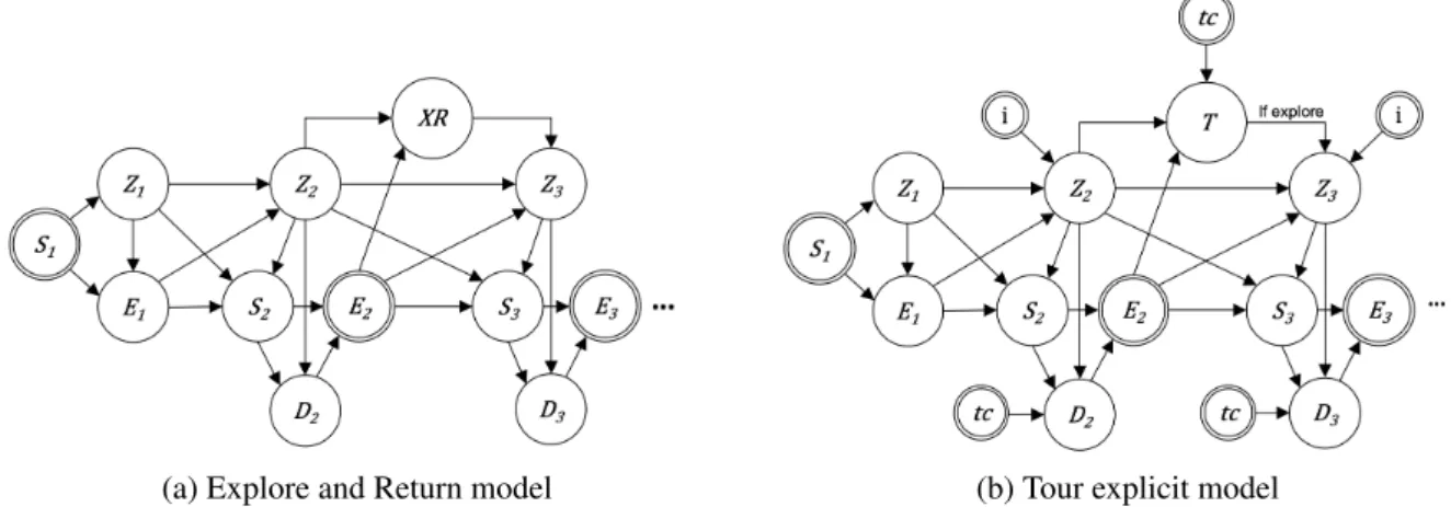
(a) Explore and Return model (b) Tour explicit model
Figure 1: Graphical representation of modified Markov models for individual travel demand. Random variables are represented as circles, deterministic variables are represented as double circles, and the arrows indicate their dependencies. (a) Explore & Return model (b) Tour explicit model
4.3. Tour Explicit Model
290
The Explore/Return (XR) variable models indirectly the daily individual tour networks. Alter-
291
natively, we can introduce a random variable that directly reconstructs tour networks. This is the
292
essence behind the Tour explicit (TX) model. We first define a way to encode tour networks as
293
sequences of digits, where each digit corresponds to a stay-zone. In this way, different stay-zones
294
are mapped to different digits while same stay-zones are mapped to the same digit. For instance,
295
the sequence 01020 refers to an individual that started the day at location 0, then moved to lo-
296
cation 1, back to location 0, then to location 2, and finalised the day back at the initial location
297
0. In this example, the semantics behind this type of network might refer to the activity chain
298
[Home-Work-Home-Shopping-Home], where it is assumed that each type of activity is done at a
299
different location. Secondly, we introduce the random variableT that models the next digit in the
300
sequence given the current tour-code sequencetc, the current time and the current stay-zone. This
301
isP(T|Zk,Ek,tc). The implementation works as follows, a digit is sampled fromT. This digit can
302
be either any of the digits already in the currenttcor the next digit to the highest one intc. If the
303
digit sampled is not intcthen it is interpreted as an explore transition step (similar to the Explore
304
and Return model); else, the transition is done directly to the stay-zone corresponding to the digit
305
sampled. There are two other changes in the conditional probabilities. One is to make the explore
306
transition probability dependent additionally oni, which is a counter for the number of stay-points.
307
The other one is to make stay-zone duration (D) dependent on the current tour sequencetcas well.
308
These augmented conditional distributions areP(Zk+1|Zk,Ek,T,i) andP(Dk|Zk,Sk,tc) respectively.
309
Fig. 1b shows the graphical representation of the Tour explicit model.
310
5. Types of urban travellers
311
A complementary strategy that we investigated was the idea of learning a generative model for
312
each type of traveller rather than a general model for the entire population. The intuition behind
313
is to keep the randomness of the sampling process constraint to the space of a more homogeneous
314
group of travellers, avoiding in this way the generation of synthetic travellers that are a mixture of
315
different types.
316
To obtain different types of travellers, traditionally, travel demand is segmented according to
317
socio-demographic information (e.g. worker, student and non-worker) (Kutter, 1972) and in more
318
recent studies, according to certain personal attributes (e.g. licence ownership, rail discount card
319
ownership) (Schlich and Axhausen, 2005) and activity chains (Schlich and Axhausen, 2005; Jiang
320
et al., 2012). Unfortunately, neither personal attributes nor activity labels are often available in
321
mobile phone datasets. The travel demand segmentation, hence, requires to be done using only the
322
intrinsic mobility patterns in mobile phone data.
323
A straightforward option is to segment travellers based on their mobility tour networks. How-
324
ever, this approach carries two main drawbacks. First, there might be too many different types
325
of tour networks (e.g. +100), resulting in not enough data to populate the required distributions.
326
Second, tour networks do not necessarily distinguish different types of travellers. Take for instance
327
three different individuals: Alice, which starts her day at home, goes to work at 9 am, then at 6 pm
328
goes to the gym, followed by dinner at 8 pm and returning home at 10 pm. Alice’s tour network
329
code would be ”01230”, given that each activity has its unique location; Bob, also starts his day
330
at home, goes to work at 9 am, does some shopping at 7 pm, and returns home at 9 pm. Bob’s
331
tour network would be ”0120”; and Carlos, who starts his schedule at home, goes to the park at
332
noon, has lunch at a cafe at 2 pm and comes back home at 4 pm. Carlos’ tour network would be
333
”01230”, which is the same as Alice. If we would manually cluster them into two groups, a more
334
sensible choice would be to put Alice and Bob together (since they are both commuters with extra
335
activities after work), and Carlos in the other group (a non-worker group).
336
In order to achieve a more meaningful segmentation of travellers based only on their mobile
337
phone traces, we have previously proposed in Anda and Ordo˜nez Medina (2018) clustering a set
338
of variables that capture different traits of travel behaviour to obtain different types of travellers:
339
Stay-points mean duration. The average duration across all stay-points of a user during one day.
340
It is a proxy of the number of trips done by a person.
341
Stay-points standard deviation duration. The standard deviation of the duration across all stay-
342
points of a user. It differentiates users with homogeneous activity durations from users with non-
343
homogeneous activity durations.
344
Bias morning-night. The difference between the average of stay-points durations before noon and
345
the average of stay-points durations after noon. It describes whether a person is an early traveller
346
or a late traveller.
347
First departure. Time of the day in which the user performs his/her first trip departure.
348
Last arrival. Time of the day in which the user made his/her last arrival.
349 350
A couple of clustering algorithms were tested, from which HDBSCAN (Campello et al., 2013)
351
resulted in more representative clusters. From the obtained clusters, we can proceed to train inde-
352
pendent generative models.
353
6. Evaluation
354
6.1. Dataset
355
The proposed methodology was tested using user-aggregated data from one of the major mo-
356
bile network operators in Singapore. Raw mobile phone data is processed and converted to indi-
357
vidual stay-point data by the operator. The histograms required for this study are aggregations on
358
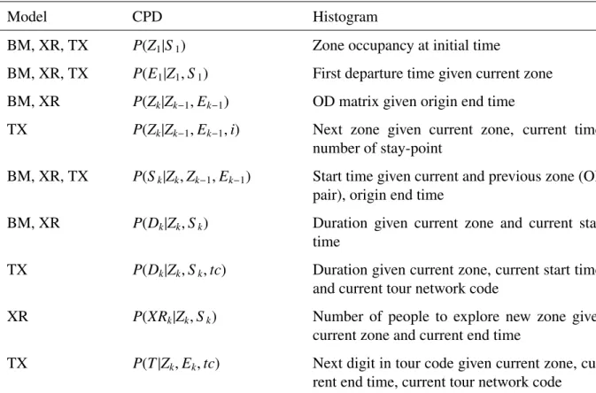
top of the stay-point data. Table 1 specifies each of the histograms required, their corresponding
359
conditional probability distribution (CPD) and the model(s) they correspond to. All histograms
360
relate to the 18th April 2017, a typical working Tuesday. They account for 50% percent of the
361
total population (around 2.8 million users). In terms of the spatial resolution, they are aggregated
362
into subzone planning boundaries3, which are divisions within a planning area centred around
363
a focal point such as a neighbourhood centre or an activity node and with an average coverage
364
of 2.3 squared km. A total of 315 subzones which cover the extension of the main island were
365
considered. As for the temporal resolution, all histograms were aggregated on an hourly basis.
366
Histograms depending on the type of traveller were aggregated considering the 16 different
367
clusters (7 related to commuters and 9 to non-commuters) reported in Anda and Ordo˜nez Medina
368
(2018).
369
6.2. Experiments
370
The models proposed were trained on aggregates corresponding to 70% of the data and used
371
to generate one million samples (i.e. synthetic travellers). We compared a series of distributions
372
of the generated samples against the distributions of the 30% left out sample. We replicated each
373
experiment setting five times in a Monte Carlo cross-validation (MCCV) way to report on the sen-
374
sitivity of different data partitions. The seven different target distributions are: start time, duration,
375
subzone (i.e. location), distance travelled, number of trips, tour network distribution, semantic
376
similarity. If there is a close match on those distributions, we conclude that the model is capable
377
of producing synthetic travellers that behave similarly to the real ones.
378 379
Following are the different configurations tested:
380
1. Baseline Markov model (BM)
381
2. Explore and Return model (XR)
382
3. Tour explicit model (TX)
383
4. Explore and Return for each cluster of travellers (XR-C)
384
5. Tour explicit for each cluster of travellers (TX-C)
385
3https://data.gov.sg/dataset/master-plan-2014-subzone-boundary-web
Table 1: Types of histograms required (BM: Baseline Markov model, XR: Explore and Return, TX: Tour explicit)
Model CPD Histogram
BM, XR, TX P(Z1|S1) Zone occupancy at initial time
BM, XR, TX P(E1|Z1,S1) First departure time given current zone BM, XR P(Zk|Zk−1,Ek−1) OD matrix given origin end time
TX P(Zk|Zk−1,Ek−1,i) Next zone given current zone, current time, number of stay-point
BM, XR, TX P(Sk|Zk,Zk−1,Ek−1) Start time given current and previous zone (OD pair), origin end time
BM, XR P(Dk|Zk,Sk) Duration given current zone and current start time
TX P(Dk|Zk,Sk,tc) Duration given current zone, current start time, and current tour network code
XR P(XRk|Zk,Sk) Number of people to explore new zone given current zone and current end time
TX P(T|Zk,Ek,tc) Next digit in tour code given current zone, cur- rent end time, current tour network code
6.3. Validation metric
386
We use theW1 Wasserstein metric (or Earth Mover’s Distance) to measure the distances be-
387
tween a series of target distributionsqand the obtained onesp. TheW1 metric can be interpreted
388
as the minimum amount of work needed to transform one pile of dirt (i.e. one distribution) into
389
another one. Hence, this minimum amount of work can be regarded as a metric to compare how
390
much two distributions differ. In a more formal way, and considering the Kantorovich formulation
391
from theoptimal transport problem(Levina and Bickel, 2001), given two random variablesXand
392
Y with probability distributions p andq respectively, we want to find the optimal transport map
393
f∗, which is a joint distribution of XandY, that minimises the expectation under f of an arbitrary
394
distance function betweenXandY. This is,
395
W1(p,q)= min
f
"
Ef[d(X,Y)] : (X,Y)∼ f, X ∼ p, Y ∼q
#
(10) As our target and generated distributions come from histograms, we can consider the discrete
396
case for the Wasserstein metric and express the expectation in eq. 10 as,
397
Ef[d(X,Y)]=
n
X
i=1 n
X
j=1
fi,j d(xi,yj) (11)
where we assume that the support ofX andY is of same sizen. It is also more clear now how the Wasserstein metric relates to an energy function, where fi,j is the mass we want to transport andd(xi,yj) is the cost or distance required to move that mass. Furthermore, if we consider the constraints:
n
X
i=1 n
X
j=1
fi,j = 1, fi,j ≥0 ∀i, j,
n
X
i=1
fi,j =qj,
n
X
j=1
fi,j = pi (12) then eq. 11 can be expressed as a linear program (Rubner et al., 2000).
398
In contrast to other ways of comparing two distributions (e.g. Jensen-Shannon divergence,
399
Kolmogorov-Smirnov test), the Wasserstein metric takes into consideration an arbitrary distance
400
function for the support of the distribution. This distance function can be chosen freely depending
401
on the type of distributions to compare. In our case, we are handling different types of support:
402
categorical (e.g. type of tour network), numerical acyclical (e.g. hourly duration) and numerical
403
cyclical (e.g. hour of the day). As a way to provide one distance metric for all, and following
404
Bindschaedler and Shokri (2016), we choosed(xi, yj) = 1i,j. This choice yields the following
405
closed form solution for the optimisation problem in eq. 10,
406
W1(p,q)= 1−X
i
min{pi, qi} (13)
In order to compare the different experiments using a single score, we define the one-day
407
mobility population accuracy score as,
408
accscore(pop)= 1−1 K
K
X
k=1
W1(p(k), q(k)) ∗100 (14) whereK is the total number of distributions to compare, p(k)is thekthobtained distribution from
409
the generative model andq(k)its corresponding target distribution. SinceW1is bounded [0,1], the
410
range of eq. 14 is [0,100], where 100 is a perfect score for the mobility population. We simplify
411
the one-day mobility population accuracy score by substituting eq. 13 as follows,
412
accscore(pop)= 100 K
K
X
k=1 n
X
i=1
min (p(k)i , q(k)i ) (15) Additionally, we were also interested in validating a notion of semantic similarity following
413
Bindschaedler and Shokri (2016) and Ouyang et al. (2018). Semantic similarity arises from the
414
idea that even though two different mobility traces might differ geographically, they could be
415
semantically similar if the purpose of the visits and the way they happen are similar. However, the
416
difficulty in doing so is that mobile phone data commonly lacks labels about the type of activities
417
or the type of travellers. To this end, we make use again of the five temporal variables in section
418
5 used to characterise different types of travellers. The objective is to compare how similar is
419
the distribution of points in the 5-dimensional space of the generated population to the real one.
420
The closer the models are to the target, the closer they are able to generate semantically similar
421
mobility traces.
422
We then define semantic similarity (SS) as:
423
S S = 1−W1(pclust, qclust)∗100 (16) Where, pclust andqclust are the distribution of clusters of the 5-dimensional space of the target
424
population and the model distribution respectively. Clusters for the generated populations can be
425
found in a supervised-learning way (e.g. using K-nearest neighbours) by using the centroids of the
426
clusters of types of travellers obtained as labels.
427
6.4. Results4
428
6.4.1. Agent-related distributions
429
Fig. 2a shows the distribution of the number of trips performed by an agent during a day.
430
The x-axis indicates the number of trips, and the black coloured bars indicate the 30% hold out
431
sample — the target distribution. We can observe that both the BM and the XR model are unable
432
to emulate the 2-trips peak and instead over-generate agents with 3 to 5 trips when compared to the
433
target distribution. XR-C model, on the other hand, overshoots 1-2 trips and misses to generate
434
enough agents with 3-4 trips. As for both TX and TX-C, the match with the target distribution
435
becomes closer.
436
As mentioned previously, one of the disadvantages of using Markov models is the lack or
437
inefficiency in handling long term dependencies, thus, resulting in non-realistic daily tour networks
438
for every agent. In fig 2b, we show how our models perform in terms of the top 12 daily tour
439
network distributions. Here, the x-axis indicates the numerical code for each of the top 12 tour
440
networks. As expected, the BM model shows a poor performance without being able even to
441
generate the home-work-home (i.e. 010) network. The XR model starts capturing the return-
442
to-home behaviour for the tour networks ending in 0. As we analyse the results for the rest of
443
the models, we can see that the XR-C outperforms the version without clusters, TX yields better
444
results than the XR-C, and finally, the TX-C shows the best results out of all models. For a
445
quantitative comparison, we present the W1 metric results in table 1. On which, we have extended
446
the evaluation of the daily tour network distribution to include the top 100 networks which account
447
for more than 85% of all tour networks presented in the hold out 30% sample.
448
4The resulting graphs and analysis were done from a single Monte Carlo experiment since we found almost no meaningful variation across the different data partitions. Nonetheless, the average results of all Monte Carlo experi- ments along with a 95% confidence interval are reported in table 2.
(a) Number of trips per agent distribution
(b) Daily tour network distribution
Figure 2: Agent-related distributions validation. (a) Number of trips per agent distribution (b) Daily tour network distribution
6.4.2. Temporal-related distributions
449
Fig. 3a shows the results for the start time distribution of stay-points. The x-axis represents the
450
hour of the day in which agents start their activity. The black-coloured plot represents the target
451
distribution, while, the other colour plots represent the results of each of the models evaluated.
452
Similarly, in Fig. 3b we present the results for the duration distribution of stay-points. Here the x-
453
axis represents different durations, from 0-hour duration (i.e. less than 1-hour duration) to 20-hour
454
duration of the activities performed by the agents at a specific location. For both cases, we can
455
identify a close match of all models, including the BM model. This means that the fundamental
456
structure of the BM model, on which the other models are built on top, effectively captures the
457
sequence of transitions in spatio-temporal trajectories. For a quantitative comparison, table 1
458
shows the W1 metric for both distributions.
459
(a) Start times distribution (b) Durations distribution Figure 3: Temporal distributions validation. (a) Start time distributions (b) Durations distribution
6.4.3. Spatial-related distributions
460
We are also interested in validating whether the agents created are in the correct locations at
461
the correct times as compared to the real population. For this, we calculated the W1 metric of the
462
distribution of agents in each subzone, for every hour of the day. Fig. 4a shows how this distance
463
(or error) develops across the day for the different models proposed. We can notice that the BM
464
model outperforms the other ones with a lower hourly error throughout the day. It gets clear what
465
is the trade-off between the BM model and the other models. The BM model results in more
466
accurate spatial distributions of locations in exchange for unrealistic individual tour networks.
467
The XR model, on the other hand, improves on the tour network distribution at the cost of lower
468
accuracy in the spatial error distribution (up to∼4% error). For the other models, as the complexity
469
increases, the spatial error distribution starts converging on average to the baseline Markov error,
470
while keeping more accurate tour network distributions. Additionally, we have also included the
471
baseline Markov spatial error when compared to the training data (grey plot) to further analyse
472
how the spatial error is decomposed in the models. The validation of the baseline Markov model
473
against the same training data tells us the part of the spatial error that comes from the dynamics
474
of the Markov model and the discretisation of the time variables (i.e. model error). This allows us
475
to identify the spatial error that comes from validating against new data, regardless of the model
476
(yellow area). For our proposed model, we can then divide the spatial error in three components.
477
The first one the model error (∼0.6%, grey area), the second one the error coming from validating
478
in new data (∼ 0.9%, yellow area), and the third component, the error that comes from the added
479
mechanisms to mitigate the first-order Markov property. In fig. 5 we present how the spatial error
480
is distributed geographically (by planning subzones) at 16:00 hrs, which is the hour of the day with
481
the highest spatial error. From the colour gradients, red means more individuals in the subzone
482
than in the validation data, while blue means less individuals in the subzone than in the validation
483
data. In general, we can notice that at 16:00 hrs the XR and XR-C models locate more agents in
484
some residential areas than required and less in the downtown area. This means that the agents
485
are returning home earlier than expected. One possibility is that the agent correctly draws a return
486
after a work lunch break for instance, but instead of returning to the office location there is some
487
bias to return back home. In the TX and TX-C models, this error is mitigated through a more
488
direct way in how the tour networks are constructed. In table 1, we report the 24-hours average of
489
the W1 metric for each of the models.
490
Fig. 4b shows the results of the total distance travelled. This distance is calculated as the sum
491
of the euclidean distances between each of the centroids of the subzones visited. The x-axis refers
492
to the total distance calculated in km. We notice that the baseline model performs poorly, with
493
the mode of the distribution centred around 20 km instead of 7 km, where the target distribution
494
mode is located. All the other models show better performance as their shape becomes closer to
495
the target. To calculate the W1 metric, we discretised the distribution into an 80 bins histogram
496
and report the results in Table 1.
497
(a) Spatial error distribution (b) Distance travelled distribution Figure 4: Spatial distributions validation. (a) Spatial error distribution (b) Distance travelled distribution
Figure 5: Spatial distribution error at 16:00 hrs.
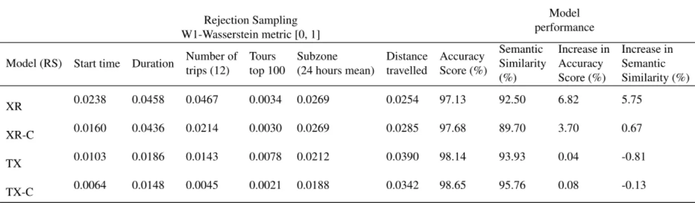
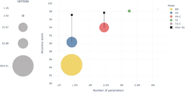
6.4.4. Accuracy score and semantic similarity
498
Aside from the W1 metric for all distributions, table 1 also presents the one-day mobility pop-
499
ulation accuracy score, the semantic similarity metric and the number of parameters for each of
500
the models. The accuracy score was computed taking into account start time, duration, top 12
501
number of trips, top 100 tour networks, 24-hr average subzone, and distance travelled distribu-
502
tions. We can see that all models outperform the BM model in terms of the accuracy score and
503
semantic similarity. Another observation is that as the model complexity increases the accuracy
504
score and semantic similarity also increases, achieving the maximum average accuracy (98.59%)
505
and maximum average semantic similarity (95.90%) with the Tour explicit with clusters model.
506