Dissertation submitted to the Combined Faculties for the Natural Sciences and for Mathematics of the Ruperto-Carola University of Heidelberg, Germany for the degree of Doctor of Natural Sciences

submitted to the

Combined Faculties for the Natural Sciences and for Mathematics of the Ruperto-Carola University of Heidelberg, Germany

for the degree of Doctor of Natural Sciences

presented by

Master of Science: Heiko Eisele

born in: Stuttgart, Germany

Oral examination: 12/18/2002

and evaluation in X-ray CT images

Referees: Prof. Dr. Fred Hamprecht Prof. Dr. Kurt Roth

Die R¨ontgencomputertomographie findet zunehmend Einsatz in der industriellen Qualit¨atskontrolle. Es ist jedoch eine grosse Herausforderung, sie in der vollautoma- tisierten Fertigung zu verwenden, da dies u.a. robuste Volumenbildverarbeitung auf verrauschten Bildern erfordert. Die vorliegende Arbeit pr¨asentiert Methoden zur au- tomatischen Detektion und geometrischen Beschreibung von Defekten. Die Erken- nung der Defekte beruht auf einer statistischen Grauwertanalyse. Im Anschluss an die Detektion werden defekte Voxel gruppiert um Form und Gr¨osse der zugeh¨origen Materialfehler zu bestimmen. Es werden Ergebnisse in der Poren- und Rissdetektion von Stahlteilen gezeigt.

Abstract

X-ray computed tomography gains increasing popularity for industrial quality in- spection tasks. It is a challenge however to use it in a fully automated assembly line, which requires robust algorithms for volumetric image analysis on noisy data.

This work provides methods for the automatic detection of defects and their geo- metric description. The approach will be based on spatial statistical analysis of the voxel structure to determine the presence of a defect. Once detected, defect voxels will be clustered to determine shape and size of the associated material faults. The effectiveness of the method will be shown on pores and cracks in steel parts.

1 Introduction . . . 1

2 Industrial Applications of CT . . . 2

3 Review of related work . . . 4

4 CT Fundamentals . . . 5

4.1 Data Recording . . . 5

4.2 Image Properties . . . 6

4.2.1 Artifacts. . . 6

4.2.2 Noise. . . 6

4.3 Processing time . . . 6

5 Volume image processing . . . 9

5.1 Detection. . . 9

5.1.1 Segmentation. . . 9

5.1.2 Feature extraction. . . 9

5.2 Outline of the main contribution of this work. . . 10

6 Defect detection. . . 11

6.1 Object and background. . . 11

6.2 Classifying regions as defect. . . 14

6.3 Improvements for small low-contrast defects . . . 14

6.3.1 Defect enhancement . . . 16

6.3.2 Statistical model. . . 17

6.3.3 Error Propagation. . . 17

6.3.4 Results . . . 21

6.4 Complexity and performance . . . 26

6.4.1 Complexity. . . 26

6.4.2 Performance. . . 27

6.4.3 Outlook: performance improvements . . . 28

7 Feature extraction . . . 29

7.1 Ellipsoids. . . 30

7.2 Spherical Harmonics . . . 30

7.2.1 The mathematical model. . . 30

7.2.2 Adaption to real data. . . 33

7.2.3 Results . . . 35

8 From the raw data to the inspection protocol. . . 39

9 Conclusion and outlook . . . 40

A Calculations and proofs . . . 43

A.1 Error propagation . . . 43

A.2 The variance of a squared gaussian random variable . . . 44

B Algorithmic details . . . 45

B.1 3D labeling . . . 45

C Software architecture. . . 47

C.1 Technical realization . . . 47

D Flowchart summary. . . 52

1 Introduction

X-ray computerized tomography is a powerful technique to image internal features of industrial parts. It thus attracts the interest of quality control engineers, who otherwise rely on less universal non-destructive testing methods such as ultra-sound or eddy current. In many cases they even have to revert to destructive techniques, which are elaborate and can access internal features at selected positions only. X- ray CT on the other hand generates a volume image of the entire object down to resolutions of a few µm easily achieved with modern systems.

This work contributes to automatic processing of X-ray CT data with the pur- pose of defect detection. While known techniques in that field primarily have been developed for conventional 2D X-ray imaging [1,2,3,4], this paper provides algo- rithms, which define pixel neighborhoods in all three coordinate directions.

The report is organized as follows: Section 2 gives a brief overview of typical defect detection tasks approached through X-ray CT. Section3discusses previously reported work on related techniques in the field of 2D X-ray image evaluation. We proceed in section4with a quick summary of technical aspects of X-ray CT to give some insight into specific challenges faced by image processing. Section 5 puts our work in the context of volume image processing techniques used in other areas such as medical research. Sections 6 and 7 detail the main contributions of this work.

Section 6 is concerned with the detection of defects, whereas section 7 provides techniques to extract their features such as size and shape. The main part of this paper concludes in a summary and outlook. We designed a GUI-based software application that serves as an interface to parameterize and apply the algorithms to arbitrary CT-data. We will describe some key aspects of that work in the appendix.

2 Industrial Applications of CT

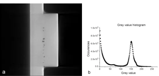
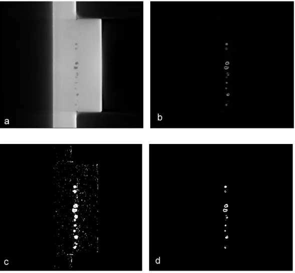
The detection of pores, contraction cavities, cracks and inclusions are important tasks in industrial quality control. Pores and contraction cavities are material faults found in welds and castings (see fig. 1(a) and (b)). While it is technically often not possible to produce parts free of defects, their type and extent determine whether the part has to be classified as good or bad. In addition, a detailed spatial distribu- tion of the defects obtained through CT provides valuable information for process engineers. A CT-system could be used for mechanically supervised monitoring of the manufacturing process. This requires fully automatic evaluaton of the images which is the objective of this work.

Fig.1(c) shows a crack running through a steel part. While cracks are the most critical of all defects, they are extremely hard to detect. The visibility of a defect in an X-ray image primarily depends on two factors: the difference in absorption with respect to its environment and its size. Since cracks are very narrow, they offer a minimum of contrast and in many cases can’t be resolved at all.

Another class of defects are inclusions. Fig.1shows an inclusion that had devel- oped during the welding process. Its contrast is very weak since it consists of slag that has an absorption very similar to the surrounding material.

A further application of industrial X-ray CT is the measurement of inner ge- ometries. However, most current applications can be found in the areas of defect detection discussed in the previous paragraph. For that reason and due to the fact, that defect detection can be approached in a more general manner we chose to focus our efforts on that field.

Fig. 1: Examples for industrial inspection tasks. (a) Pores and contraction cavities in castings, (b) and (d) welding defects, (c) crack.

3 Review of related work

Defect detection requires a decision whether individual voxels differ significantly from the background. Early applications have used median filtering techniques to obtain a background image and applied a threshold to the difference image [1]. To distinguish between constructive features and defects, they adapted the filter mask to the object geometry. Each object requires a learning stage in which the best masks are selected either manually or automatically. This requires a defect-free part, how- ever, which is not always available. The mask selection has been improved in [3], but the method still has difficulty with low-contrast defects typical in X-ray CT images (see fig. 4). Gayer et al. [2] used high-pass or first derivative filtering to identify potential defects. True defects were subsequently identified via template matching.

This technique takes advantage of neighborhood information but requires a priori knowledge about defect shapes. Alternatively, the authors computed a background image by interpolating between pixels that had been marked as intact and applied a threshold to the difference image. However, this still has the previously mentioned disadvantages, i.e. poor performance on low-contrast noisy defects.

A recent approach uses both spatial variance and spatial contrast and applies fuzzy reasoning to distinguish between defect and background [4]. This technique does not require heuristic threshold parameters since these are estimated in the training process.

Our method will detect defects by evaluating the deviation not of singular voxels, but structural deviations from the background. This approach is particularly suitable for low-contrast planar defects such as cracks, that are difficult to detect with other methods. However, the technique works on more compact defects such as pores and contraction cavities as well.

4 CT Fundamentals

This section gives an outline of the data aquisition process in X-ray CT, i.e. data recording and geometry reconstruction. Data recording refers to the physical collec- tion of data through an X-ray detector whereas reconstruction processes those data to obtain a volume model of the object.

4.1 Data Recording

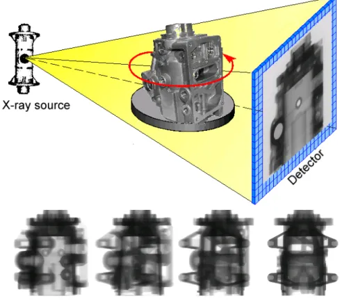
Fig. 2: During a CT recording, several hundred individual images are taken from different angles and used to reconstruct the volume information. Provided by Dr.

Andreas Siegle, Robert Bosch Corp.

Fig.2illustrates the principle of X-ray CT data recording. An X-ray source irra- diates an object whose image is recorded by a detector array. The turntable rotates stepwise to record object images from different angles. A CT recording typically consists of several hundred individual projections.

During image reconstruction, individual images obtained from different angles are processed to yield a 3D volume image of the object. The basic algorithm to

perform this task is the so-called Feldkamp-Algorithm [5]. This technique has been modified for increased performance or better image quality in a number of articles, e.g. [6].

4.2 Image Properties

The reconstructed images have a number of properties characteristic of X-ray CT- data. The major challenges image processing algorithms have to cope with are arti- facts and noise.

4.2.1 Artifacts We only quote the most salient artifacts that limit defect detec- tion. The so-called cupping artifacts make the absorption appear stronger near the boundaries than in the interior of the object, even if it is homogeneous (see fig. 3).

We will model defect-free image data based on a local training region. The non- homogeneity caused by the cupping artifact will limit the algorithm’s performance near the object boundaries. The physical cause for the cupping artifact lies in the non-linearity of the absorption as a function of the beam energy and is discussed in more detail in [7].

Edge artifacts appear as a halo near the object boundary making small defects difficult to detect, especially close to strongly absorbing materials (fig. 4).

4.2.2 Noise As most defects manifest themselves in a deviation of the absorption from that of homogeneous material, their detectability is limited by noise (see fig.4).

In section 6.3 we will perform defect detection by evaluating the significance of the deviation of groups of pixels from the background. This will involve estimating the covariance matrix

Cov_g =h g_(i,j,k)−g¯

, g_(i0,j⁰,k⁰)−g¯

i (1)

where we average across the homogeneous area of the image, and subsequently estimate the noise after performing certain neighborhood operations. Details of that procedure including the quantification of the noise parameters will be presented in section 6.3.

4.3 Processing time

Image processing should take no longer than data recording and reconstruction, which require approximately 20−30 min each for a 512×512×512 volume. The bottleneck in data recording is the integration time on the detector to obtain a sufficiently large signal-to-noise ratio.

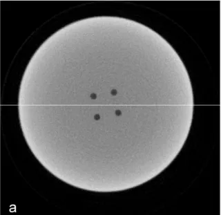
Fig. 3:Cupping artifact. The grey values in the middle of the object are smaller even though the X-ray absorption is constant throughout the object. (a) Grey image, (b) cross-section.

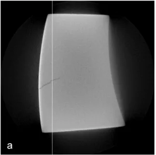
Fig. 4: Noise. The crack is hard to detect due to its low contrast. (a) Grey image, (b) cross-section.

5 Volume image processing

Currently most applications of volume image processing can be found in medical fields such as cancer diagnosis or brain research [8,9,10]. This section gives a brief overview of techniques that can also used for industrial image processing.

5.1 Detection

Defect detection means assigning voxels to two kinds of classes: intact or defect.

This decision will be based on thresholding techniques which are basically classified as point-dependent or region-dependent. Point-dependent techniques take into ac- count a pixel’s grey value only whereas region-dependent methods use neighborhood information. Both techniques may be applied locally or globally [11].

5.1.1 Segmentation Segmentation refers to the process of extracting connected regions with similar properties. This is a common problem in brain research, where the goal is to obtain a functional map of the brain [9,10]. Typical techniques in this field are so-called region growing algorithms, where starting from distinct seed points, regions with similar grey value structure are extracted. We will use this general technique to distinguish between defects and constructive object features.

5.1.2 Feature extraction In feature extraction we will compute parameters de- scribing size and geometric defect properties. Known methods can be divided into two main categories: model-based (parametric) and non-parametric.

An example of non-parametric techniques are active contours or ’snakes’ intro- duced in [12]. The physical analogy of an active contour is a ring of masses connected by springs. The masses also experience a force derived from a grey image. A com- mon method to calculate this force is to equate the grey value of an image with the potential energy. The snake will then change shape to reach a state of minimum energy. This method has a drawback regarding noisy images: The snake might get stuck in a local minimum. As a solution Velasco et al. introduced so-called Sandwich Snakes [13]. Here two snakes are initialized, one inside and one outside the object.

The interaction among them will force them to converge on the true object bound- ary. Raisch et al. [14] applied a special energy term with reduced noise to avoid being trapped in local minima in the first place.

While snakes are very useful in boundary extraction and have been widely ap- plied, they do not directly yield object features. Model-based approaches yield object properties directly and can be adapted to the desired level of detail. Examples of

prototypes are ellipsoids [15] and spherical harmonics [16]. In [16], the use of mo- ments for shape characterization is discussed as well.

In our work we decided to use a model-based approach, since lower order shape parameters are usually sufficient for defect characterization.

5.2 Outline of the main contribution of this work

Section 6 deals with the detection of defect voxels. For an object composed of one material, we first perform a grey value segmentation using a global threshold, which is determined from the histogram. This distinguishes between material and air. In a second step, we use topological properties of the segmented regions to distinguish between defects and background.

In the subsequent section we suggest an alternative to using a global threshold as a criterion for binarization. We apply structure enhancing operators locally and regard defects as outlier structures from the estimated background. As we will show this technique performs better on low-contrast noisy images with varying intensity.

In contrast to previously reported approaches, it uses both neighborhood informa- tion and subsequent statistical testing for defect detection. The detection threshold can then be chosen independently from the image content.

Section 7 determines the shape characteristics of the defects based on the de- tection result. We will suggest two model-based approaches: The first one describes defects with ellipsoids. This seems appropriate since in many cases one is interested in the main axes of a defect and their ratios. The second approach uses spherical harmonics, which allows to distinguish among more complex shapes. This model is very flexible in the sense that it can be adapted to the level of shape details one is interested in.

Section 8 recapitulates the key accomplishment of this work, i.e. to generate a defect protocol based on raw CT-data. The main part of this thesis concludes with a summary and some proposals for future work.

6 Defect detection

Defect detection refers to the process of classifying voxels as either intact or defect.

We first need to discard all voxels that are not an integral part of the object, such as the air in the environment or in a drillhole. This discrimination is accomplished by means of a threshold, the choice of which is documented in section 6.1. Section 6.2 describes how we distinguish between inclusions and air. Finally, section6.3 details our attempt how to detect more subtle defects that are not found by a simple thresholding operation.

6.1 Object and background

The simplest possible method for fault detection is to classify each single voxel of the raw imageg(i, j, k) as defect or intact according to the following criterion:

– voxel intact if g_(i,j,k) > t, – voxel defect if g_(i,j,k) < t,

where t is some threshold within the dynamic range of the image (0...255 in our examples). In the sense of [11], this method is global point-dependent.

Commonly used threshold selection techniques model the grey value distribution g(x) as a sum of Gaussian components, see (see [11]):

f(x) = X

i

p_i σ_i√

2πe⁻

(x−mi)2 σ2

i (2)

A voxel is then assigned to the class with the highest probability density. This tech- nique is known in the literature as mixture density modeling. Known mixture density decomposition algorithms are the MF-Estimator [17,18], and the generalized mini- mum volume ellipsoid (GMVE) [19]. These techniques estimate the parameters of each cluster by iterative refinement, which is a computationally expensive procedure and might even fail in the case of poorly chosen initial estimates [11]. Chang et al. [11] suggest an alternative approach: Instead of estimating the parameters itera- tively, they choose optimal initial conditions by first smoothing the histogram and then finding a window around each peak in which the distribution has zero skew- ness. The parameters are then estimated in a single step from these intervals. While this algorithm yields better performance and more accurate results than techniques using the MF-Estimator and B-Splines, the authors point out that the results will depend on the size of the filter used for smoothing the histogram (see [20] for a general discussion of B-Splines in computer vision).

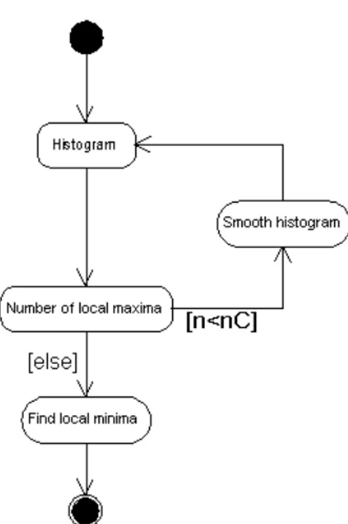
In our application, the number of components to be segmented is known a priori since it corresponds to the number of materials with different X-ray absorption (see fig. 6(b)). The leftmost flank of the histogram in fig. 6(b) is typical for X-ray CT- images and arises from artifacts during reconstruction. The main peak comes from the object itself, and the small bump in-between is due to the halo effect described in section (see section 4.2.1). Knowing the desired number of components in advance, we propose an algorithm for automatic threshold selection that does not make any prior assumptions about the particular distribution type. Our method works itera- tively but without heuristic input parameters. The histogram is smoothed iteratively with a (3×1) Binomial until the number of local maxima equals the number of ma- terial components. The local minima of the histogram are then chosen as thresholds (see fig. 6.1). Once the grey image is binarized at the resulting threshold, we obtain an approximate segmentation of the object, which classifies voxels as either occupied with material or air. This approach works well if the peaks from the different ma- terials are sufficiently distinct such that they do not coalesce. To detect defects we have to further differentiate among those classified as air. This is done by classifying their topology as described in the following section.

Fig. 5: Iterative histogram smoothing.

Fig. 6: (a) CT-image of a steel part with defects. (b) Associated histogram.

Fig. 7: (a) Smoothed histogram. (b) Fig. 6(a) binarized at the threshold extracted from the smoothed histogram.

6.2 Classifying regions as defect

Consider a single-component image that has been binarized to distinguish between material and air/vacuum (see section 6.1). This assigns both the surrounding back- ground and defects the same class, so we have to apply further techniques to extract the defects. For this purpose we apply a so-called region growing technique com- monly used in segmentation. Starting from a seed area, neighboring voxels will be included if the newly created region satifies certain homogeneity criteria based on grey values, color or texture [10,21,22]. Applications are primarily found in medical image registration. [10,9] but also in other areas such as video segmentation [21] or general applications [22].

To outline how to extract the defects in our binarized image of fig. 7(b)we first have to give some definitions:

Definition 1 Connectivity. Each voxel is connected to those of its 26 nearest neigh- bors that have the same grey value class.

Definition 2 Each connected graph corresponds to one region.

These definitions allow us to disregard all voxels that are connected to the sur- rounding atmosphere, such as drillings and channels. All remaining sub-threshold regions are classified as defects. We implement a 3D region growing algorithm that labels regions in the binarized image of fig. 7(b) to extract defects. This algorithm uses the following homogeneity criteria:

h= 1−b_(i,j,k), (3)

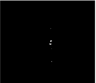
where b_(i,j,k) is the value of the binary image of fig. 7(b) (i.e. 0 or 1). The voxel (i, j, k) will join the region if and only if h= 1. Results are shown in fig.8and algo- rithmic details can be found inB.1. A schematic diagram of the detection algorithm discussed can be found in appendix D.

This technique has two limitations: firstly, defects that are just a few voxels in size are often not detected due to their low contrast (fig. 9(b)). Secondly, surface defects cannot be detected since they are labeled as surrounding air (fig. 9(a)).

6.3 Improvements for small low-contrast defects

Applying a global threshold to the image often leaves small or low-contrast de- fects undetected. In this section, we introduce methods for a local image analysis, that classifies voxels with respect to their neighborhood, rather than globally. This

Fig. 8: Fig. 7(b) after the 3D labeling. Defects are objects classified as background that are not connected to the outer image region.

Fig. 9: Examples of defects that usually remain undetected by global thresholding and 3D labeling: (a) surface defects, since they are connected to the outer image region and are thus classified as background and (b) small defects with low contrast such as cracks.

procedure comprises two steps: Firstly, defects are enhanced using special filtering techniques and secondly, a threshold is chosen based on the covariance properties of a defect-free training region.

6.3.1 Defect enhancement The key to defect enhancement is to detect oriented structures within the image. Commonly used techniques are tensorial approaches, which are discussed in [23,24,25,26]. These methods require eigenvalue computation for each pixel, which results in a computationally expensive procedure. In addition, they respond to both edges and noise. As an alternative, we suggest to simply take the square of locally averaged derivatives as an edge detector. This suppresses the noise and, at the same time, enhances pixels within areas of coherent grey value structure. The corresponding operator looks like this:

g⁰(x) =

3

X

i=1

Z

w(x−x⁰)∂g(x⁰)

∂x_i dx⁰ 2

(4) Here g(x⁰) is the grey value at pointx= (x₁, x₂, x₃) and ∂/∂x_i the derivative with respect to the i^th coordinate. w denotes a three-dimensional smoothing function (commonly a Gaussian). The discrete version of this equation is

g⁰ = (g∗f_x^p)²+ (g∗f_y^p)²+ (g∗f_z^p)² (5) where

f_x^p =B_x^pB_y^pB_z^pD_2xS_yS_z f_y^p =B_x^pB_y^pB_z^pD_2yS_xS_z f_z^p =B_x^pB_y^pB_z^pD_2zS_xS_y

(6) The filter masks are

D_2x = [ 0.5 0 −0.5 ]

S_x = [ 0.1839155 0.632169 0.1839155 ] (7) and the binomial filters B_x^p are defined as

B_x⁰ = [ 1 ] B_x¹ = [ 1 1 ] B_x² = [ 1 2 1 ]

(8) The filters with index y and z have the same coefficients and are applied in the y and z-direction, respectively. D_2xS_yS_z represents a first derivative operator in x- direction that has been optimized for isotropy [27]. Smoothing the image of first derivatives has the effect that areas with coherent linear structure are preserved, whereas noise is suppressed. Results obtained on both artificial and real data will be presented in the following section. For detection, we set a threshold above which we regard a signal as significant. This requires a statistical model and estimating parameters.

6.3.2 Statistical model The noise is correlated as will be shown shortly. We therefore model the absorptiong(x) of an intact object as locally homogeneous with added correlated isotropic normal noise. In other words, we interpret the data as realization of a stochastic process with drift (the mean is only locally constant). The covariance structure is assumed constant throughout the random field (homoscedas- ticity), and it is estimated from a homogeneous training region (see fig. 11.

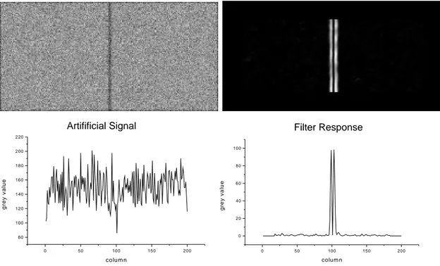
In fig. 10a CT-data of a defect part have been simulated by adding uncorrelated normal noise to a constant grey image where the voxels of the YZ plane across the center have been set to a lower grey value, and convolving the result with a (3×3×3) binomial filter to obtain correlated noise. Fig. 10b shows the result of the filtering with (5). Even though the crack in fig. 10a is clearly visible, the signal across the horizontal cross section through the image hardly shows a significant deviation from the background (fig.10c).

If g denotes the constant grey image with added uncorrelated normal noise σ and if ˜g is obtained fromg by convolution with a three-dimensional Binomialb_(i,j,k), then the variance ˜σ² of ˜g becomes

˜

σ² =σ²X

b²_(i,j,k) (9)

where the summation extends over all filter coefficients. For a (3×3×3) binomial filter the variance of the noise in fig. 10a thus becomes

˜

σ² = 0.05273σ²· (10)

Fig. 10c illustrates the difficulty in detecting low-contrast defects: A threshold of 3˜σ will barely detect the crack and, at the same time, yield a large number of pseudo errors – for a normal distributionf(x) = ^e−x

2/(2σ2)

σ√

2π we have to expect a false alarm rate of 2.7%. In a typical image with 512 ×512×512 voxels more than a million intact voxels would be classified as defect, which is unacceptable. Fig. 10d shows a far better signal-to-noise ratio. To determine an appropriate threshold, we have to know the variance of the noise in the filtered image. The next section will detail how to calculate that noise from the covariance matrix of the source image.

6.3.3 Error Propagation To determine the covariance matrix of the source image we manually select a defect-free homogeneous training region and compute the covariance matrix under the assumption that the noise is isotropic (see fig.6.3.3).

To see the effect of the filtering on the covariance matrix, we rewrite (5) as

g⁰ = (g_x⁰)²+ (g_y⁰)²+ (g_z⁰)² (11)

0 50 100 150 200 80

100 120 140 160 180 200 220

Grey Value Profile of Artificial Data

grey value

column

0 50 100 150 200

0 20 40 60 80 100

Filter Response

grey value

column

Artifificial Signal Filter Response

Fig. 10: Effect of the filtering on an artificial 3D image: (a) slice of original image:

homogeneous with crack and added correlated noise (white Gaussian noise convolved with a (3× 3×3) binomial filter). (b) Image after it has been filtered with (5);

smoothing operator: (13×13×13) binomial filter. (c) Horizontal cross section through the original image and (d) the filtered image.

Fig. 11: Analyzing the covariance structure. (a) Original image with hand-selected training region. (b) Empirical covariance vs. distance assuming isotropic noise. (c) A Gaussian fit to the empirical covariance data for small distances has a standard deviation ofσ_coh = 1.12.

where

g⁰_x =g∗f_x^p, g_y⁰ =g ∗f_y^p, g⁰_z =g∗f_z^p, (12) At point (i, j, k), we obtain

g_x(i,j,k)⁰ =

r

X

{l,m,n}=−r

f_x(l,m,n)^p g(i−l,j−m,k−n), (13)

where f_x(l,m,n)^p are the coefficients of our three-dimensional filter f_x^p. If the image is modeled as a random field as described in the previous paragraph, the variance σ_x(i,j,k)⁰² of g⁰_x(i,j,k) is

σ_x(i,j,k)⁰² =E h

g_x(i,j,k)⁰ −E

g_x(i,j,k)⁰ 2i

, (14)

where E denotes expectation. We substitute (13) into (14), rearrange terms and compute the expectation value term by term in order to obtain

σ_x(i,j,k)⁰² =

r

X

{l,m,n,u,v,w}=−r

f_x(l,m,n)^p f_x(u,v,w)^p

E

g_{(i−l,j−m,k−n)}−E

g_{(i−l,j−m,k−n)}

g_{(i−u,j−v,k−w)}−E

g_{(i−u,j−v,k−w)} (15) (see appendix A.1). Eq. 15can be rewritten as

σ_x(i,j,k)⁰² =

r

X

{l,m,n,u,v,w}=−r

f_x(l,m,n)^p f_x(u,v,w)^p Cov((i−l, j−m, k−n),(i−u, j−v, k−w)).

(16) As mentioned above, we assume the covariance function to be constant over space so that the variance at a pixel becomes

σ_x⁰² =

r

X

{l,m,n,u,v,w=−r}

f_x(l,m,n)^p f_x(u,v,w)^p Cov(l−u, m−v, n−w). (17) If we order the filter coefficients as a vector we can rewrite (15) as a bilinear expres- sion using the covariance matrix Σ_ij:

σ⁰² =f^pTΣ_ijf^p (18)

with i, j =−lmn...lmn. Since we assume isotropic noise, the expectation values of the variances σ_y(i,j,k)⁰² and σ_z(i,j,k)⁰² of g⁰_y(i,j,k) and g_z(i,j,k)⁰ are equal so that

σ⁰_z² =σ⁰_y² =σ_x⁰². (19) Let σ²_x2 be the variance of g_x⁰². By definition we may write

σ⁰²_x2 =E[g⁰⁴]−E[g⁰²]². (20)

With a few algebraic steps one can show that, if g_x⁰ is normally distributed, the variance of g_x⁰² becomes

σ_x⁰²2 = 2σ_x⁰⁴. (21)

(see appendix A.2 for more details). Finally, let σ⁰² be the variance of g⁰. Even though the derivatives of a random field are spatially correlated, the derivatives with respect to different spatial directions taken at thesame point areuncorrelated in an isotropic random field. In this case, the variance of the sum in (4) is equal to the sum of the individual variances, so that

σ⁰² = 6σ_x⁰⁴ (22)

Equations (22) and (17) relate the noise of the image filtered with (11) to the noise of the unfiltered image. This estimate of the noise in the resultant image g0 allows for the choice of a threshold at a given significance level.

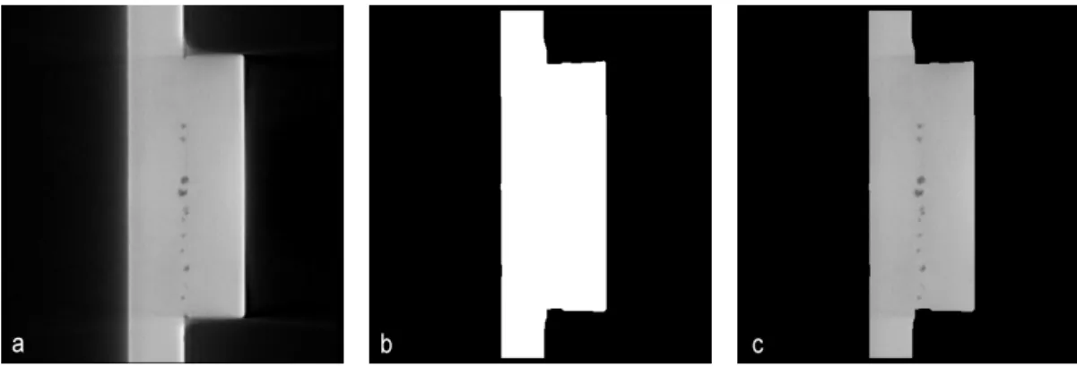
For real images we expect to improve the signal-to-noise ratio by a similar amount as shown in fig. 10. A drawback of this method is that it enhances defects as well as edges. As a workaround, we only apply this technique to the interior region of the object, which we determine by eroding the union of object and defect region (fig. 7(b) and fig. 8). Fig. 12(b) shows the region of interest, on which we detect defects. The technique will therefore still be incapable of detecting surface defects such as the one shown in fig.9(a).

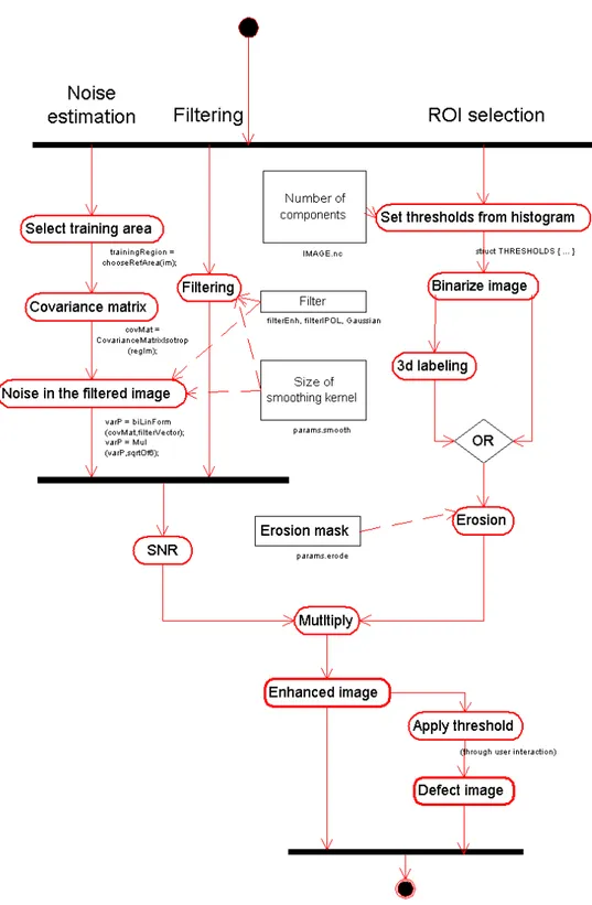
An overview of the complete procedure is given in fig. 13. The diagram shows three main execution threads: one for calculating the signal-to-noise ratio (noise estimation), one for filtering and a third one for creating the region in which defect detection is allowed (ROI selection). Sequence diagrams of the algorithm can be found in appendixD. In the next section we will present results and discuss in detail the parameters used.

6.3.4 Results Fig.14(b)shows the original image filtered according to (5) divided by the noise given by (22) or, in other words, the amplitude-noise-ratio (ANR). The ANR approximately has aχ²-distribution with three degrees of freedom. Its density is given by

fχ(x) = e^−x/2√ x 2√

2Γ(3/2) (23)

We can now select a quantile of the χ²-distribution independent of the actual image and thus can choose a detection threshold on the ANR that is universal across samples. So instead of adjusting the threshold to the image data, we trans- form the image data such that the threshold can be left constant. Fig.14(c) and (d) show the ANR binarized at thresholds 0.217 and 2.17. The parameters indicated in

Fig. 12: Region of interest (ROI) for defect detection. (a) Original image, (b) ROI (c), ROI of original image.

fig. 13 are as follows:N umber of components= 1 (determined by the object itself), Size of smoothing kernel = 1 (i.e. we don’t smooth at all and simply apply the defect enhancement filter), size of Erosion mask = 15. The size of the smoothing kernel should be adapted to the types of defects to be detected. It should be selected such that the vector normal to the defect surface points approximately in the same direction throughout the smoothing window. A larger smoothing kernel then results in a better ANR ratio. This makes the technique especially suitable for crack de- tection, as these are very low in contrast, but basically planar in shape. We already took advantage of that effect when we set the kernel size to 13 in fig. 10.

Fig. 15 shows results obtained on a real crack. The kernel size has been set to 5 in this case. While increasing the kernel size can improve the detectability of planar low-contrast defects, there is a computational cost associated with a larger smoothing window, which we address in more detail when discussing performance issues in the next section. The size of the erosion mask can be chosen depending on the covariance vs. distance function in fig. 11, though we empirically set the final value to 13σ_coh, if σ_coh denotes the range of the covariance function of the training data. For smaller values we obtain plenty of pseudo errors near the edges. From the fact that the value had to be chosen that large, we conclude that the statistical properties of the data near the edges are different from the interior, and additional effects contribute to the image properties at the borders as the discussion about artifacts (section 4.2.1) already suggested. The threshold values seem low, since we would expect a lot more pseudo defects at a ANR of 2.17. However bear in mind that the size of the covariance matrix equals the size of the filter vector f^p in (18).

In the first example we chose p = 0 so we had few data to estimate the covariance matrix and poor statistical precision. Also, since the covariances of pixels close to

Fig. 13: Overview of the complete low-contrast defect detection technique. The rect- angular boxes indicate parameters supplied by the user: the number of components, the one-dimensional filter to be applied in each direction for defect enhancement, the size of the Binomial smoothing kernel (superscript p in (5)), the amount by which the image is eroded to exclude regions close to the border from defect detection, and the threshold.

each other were predominant, we actually underestimated the noise. In the case of the crack, the size of the training region was (7×7×7) (since we used a (5×5×5) smoothing kernel). Figures 15(c) and (d) show the SNR image at thresholds 1 and 13 respectively.

Fig. 14: Panel (b) shows the signal-to-noise ratio after (a) has been filtered with (5).

(c) and (d): the image in (b) binarized at thresholds 0.217 and 2.17 respectively.

Fig.15(b) shows that there is a slight inhomogeneity of the covariance structure throughout the image, as the false alarm rate at threshold 1 appears to be bigger in the center than near the outer edges. Again, this reflects the fact that modeling the noise as homogeneous within our sample is just an approximation. Secondly, we observe an increased false alarm rate at the lower boundary of the object, which also points to the fact that our stochastic model does not adequately describe the real image near the boundaries. The range of the coherency function in this example was

Fig. 15: (a) original image, (b) after filtering with (5), (c) binarization at 1, (d) binarization at 13.

0.83, and the size of the erosion mask was set to 5.

In contrast to the technique explained in6.2, this method detects defect bound- aries. In the next section we will fit various models to those boundaries to charac- terize shape and dimension of the defects with a few parameters, but first we will give some details about the algorithm’s performance.

6.4 Complexity and performance

6.4.1 Complexity In this paragraph we will give a brief overview over the com- plexity of the computational steps involved in the algorithm. The schematic sum- mary in fig. 13 shows three main threads of the detection algorithm:

– Noise estimation – Filtering

– ROI selection

In the following we will estimate the number of arithmetic operations for the individual steps per voxel.

Noise estimation . Let C be the edge length of the training region. The covariance Covg of the grey values g_(l,m,n), where l, m, n= 0, ..., C−1, is defined by

cov_g =

g_(l1,m1,n1)−¯g

g_(l2,m2,n2)−g¯

(24) Calculating the arithmetic mean ¯g requires ∼ C³ additions. Calculating the covariance requires an additional ∼ 3C⁶ additions and C⁶ multiplications. The co- variance matrix has to be calculated only once, so the required number of additions (multiplications) per pixel is approximately 3C⁶/N³ (C⁶/N³).

Filtering Eq. 5 gives the mathematical details of this step. Smoothing (B_x^pB_y^pB_z^p) requires 3p+3 multiplications and 3padditions for each term. For the derivative part (D_2xS_yS_z etc.) 6 additions and 9 multiplications have to be performed respectively if (3×1) filters are used. This adds up to 9p+ 36 multiplications and 9p+ 18 additions.

Summing up the squares of individual terms demands an additional 3 multiplications and 2 additions.

ROI selection The computation time of this step depends for the most part on the specific image data, so its performance will be evaluated based on concrete benchmarks in the next section.

6.4.2 Performance The performance of the algorithms has been tested on the image shown in fig. 15 (image size: 511×511×280). Fig. 16 shows performance data for the three main execution threads shown in fig. 13 and discussed in the previous paragraph: noise estimation, filtering and ROI selection. The filtering is split up into the derivative (D_2xS_yS_z etc.) and the smoothing part (B_x^pB_y^pB_z^p). The bottom axis corresponds to the total number of arithmetic operations (additions plus multipli- cations). The top axis displays the total execution time on our test data set. The vertical axis represents the size of the Gaussian smoothing filter (e.g. if the num- ber given is 3, a (7×1) filter has been used (3·2 + 1 = 7)). The time scale was chosen to match the experimental performance with the number of operations for p = 6. The smoothing operation accounts for the biggest part of the total execu- tion time as the filter size is increased to achieve a better ANR (see discussion in section 6.3.4). The derivative part remains constant as the filters are not changed from those in (7). Also the parameter involved in the ROI selection has been left constant (size of erosion mask = 5). The computation time for estimating the noise is barely significant, since it does not scale with the size of the image. The next section will suggest how to optimize the smoothing procedure as it accounts for the biggest portion of the total computation time. We propose how to use more efficient filters for smoothing and will estimate the reduction in computation time upon efficient implementation.

Fig. 16: Performance of the detection algorithm. The test was conducted on the image of fig. 15 with p= 6. The computation time for the other values of pis estimated is broken down into estimating the noise, smoothing, taking the derivatives and ROI selection.

6.4.3 Outlook: performance improvements The algorithm leaves room for performance improvements at two particular points. First the smoothing filters can be implemented more efficiently: a (n×1) Binomial can be implemented efficiently as a network [28], reducing the number of operations from n−1 additions plus n multiplications to ∼ n additions. Fig. 17 shows the execution time expected upon efficient implementation of the smoothing based on the reduced number of operations just mentioned. The numbers show that there will be a significant gain for larger filter sizes, and taking the derivatives and ROI selection now are the main contributors to computation time.

This concludes the work on detecting defect voxels. We will next address, how to cluster them and extract suitable parameters for shape and size description.

Fig. 17: Hypothetical computation time, when the Binomials are implemented effi- ciently as a network.

7 Feature extraction

The previous chapter has been concerned with classifying single voxels only. For quality analysis, however, features such as defect size or orientation are important.

To extract those features we apply two model-based approaches. In this section we will use ellipsoids as prototypes and in the next section we will show how spherical harmonics can be used to fit models of arbitrary detail to the data. In any case, we first have to group voxels that belong to the same fault and determine its character- istics from there. Whether defects close to each other have to be counted as one is subject to specific inspection requirements for the product. In our example, defects closer than 2mmhave to be treated as a conglomeration of defects, for which the tol- erable extent is different than for individual defects. Within the scope of this work, there will be no distinction between those two types of defects, but conglomerates will be treated as such and not as single defects. A distance of 2mmcorresponds to 4 voxels in our image. In fig. 14d we will therefore merge regions that are closer to each other than 4 voxels. This is done by performing a (5×1) morphological dilation in the x,y and z direction. The result can be observed in fig. 18. Voxels belong to the same defect if they are connected in the sense of definitions 1 and 2. To label the regions we use our 3D labeling algorithm detailed in appendix B.1.

Fig. 18: Voxels belonging to the same defect are grouped together by performing a 5×1 morphological dilation on the image in fig. 14(d).

Having grouped voxels that are to be counted as one defect, we now have to ex- tract relevant parameters such as the exact position and the maximum and minimum extent.

7.1 Ellipsoids

To extract the features of interest we first model the object boundary as an ellipsoid.

This has an analogy in classical physics, namely calculating the tensor of inertia of a mass distribution. Its eigenvectors and eigenvalues yield the major and minor axes of the ellipsoid of inertia. For each region in fig. 18 we equate the grey values in the enhanced image (fig. 14(b)) with the masses and then determine the shape characteristics of the object via the ’tensor of inerta’. We first compute the ’center of mass’ to obtain the defect position R for each object:

R=

Pgiri

Pg_i (25) Extending the grey value-mass analogy, we can calculate the ’tensor of inertia’ for each defect:

J =







J_xxJ_xy J_xz J_yx J_yy J_yz J_zxJ_zy J_zz





 (26)

J is symmetric and has the components J_xx =X

(y_i²+z²_i)g(x_i) J_yy =X

(x²_i +z_i²)g(x_i) J_zz =X

(x²_i +y_i²)g(x_i) J_xy =X

(x_iy_i)g(x_i) J_xz =X

(x_iz_i)g(x_i) J_yz =X

(y_iz_i)g(x_i)

(27)

In the coordinate system spanned by the eigenvectors of J, the normalized tensor componentsJ_nn/P

g(x_i) (n∈ {x, y, z}) are the expectation values of the main radii of the best-fit ellipsoid to the data. Fig. 19 recapitulates the steps to obtain those radii starting from the enhanced and defect image. The related sequence diagrams are displayed in appendixDand. Fig. 20 shows results on one of the detected defects.

The data set in the left column can be well approximated by an ellipse, whereas the one in the right column exhibits significant deviations from an elliptical shape. Here a more sophisticated model is required, which will be introduced in the next section.

7.2 Spherical Harmonics

7.2.1 The mathematical model In this paragraph we provide a more general representation of three-dimensional objects that can be adapted to the level of detail required. We hereby approximate the point cloud using spherical harmonics. The

Fig. 19: Computing the principal defect axes based on the tensor of inertia.

Fig. 20: Modeling a defect with an ellipse (for each column, the figures show three orthogonal views of the same plot). Left column: the ellipse fits the data pretty well.

Right column: the points form a shape that deviates significantly from an ellipse.

spherical harmonics form a complete orthonormal set of functions in L₂(S₁) where S₁ represents the unit sphere. InR₃ they are defined as

Y_l^m(θ, φ) =Y_l^m_e(θ, φ)+Y_l^m_o(θ, φ) =P_l^m(cosθ) (cos(mφ) +sin(mφ)), m= 0,1,2, ..., l (28) whereP_l^m are the associated legendre polynomials. A linear combination of theY_l^m can describe arbitrarily complex objects R(θ, φ) in spherical coordinates:

R(θ, φ) =X

m,l

a^m_l Y_l^m_e(θ, φ) +b^m_l Y_l^m_o(θ, φ) (29) The odd functions Y_l^m_o all change sign under the transformation φ → −φ and exhibit a shape rather untypical for defects. We hence use the even part only, so our approximation becomes

R(θ, φ) =X

m,l

a^m_l P_l^m(cosθ)cos(mφ) (30) where the sum can be truncated according to the level of shape detail one is interested in. Fig. 21 shows the even part of a few of the basis functions. The next section addresses how to estimate the coefficients in (30) based on the real data.

7.2.2 Adaption to real data Saupe et al. used spherical harmonics to extract features from 3D models that could be used to retrieve similar objects from a database [16]. They estimated the coefficients of the expansion via a spherical FFT algorithm. We will take a different approach, i.e. we will use a least squares esti- mator to fit each model to our data. Given a set of points in spherical coordinates (r_i, θ_i, φ_i, g_i), whereg_i denotes the grey value, we need to find the coefficients in (30) such that

S:=X

i

g_i² r_i−X

m,l

a^m_l Y_l^m_e(θ_i, φ_i)

!2

−→min. (31) The sum represents the average radius as a function of (θ, φ). Eq. 31requires

∂S

∂a^m_l = 0 (32)

for all a^m_l to be considered. Equation 32 is a system of linear equations which can be expressed as:

G·a=d (33)

If we truncate the sum in (32) after n terms, G is an n×n matrix with the entries Glm=

N

X

i=1

g_i²fl(θi, φi)fm(θi, φi) (34)

Fig. 21: A few representatives of even spherical harmonics: (a) Y₀⁰_e. (b)Y₂⁰_e. (c)Y₄²_e

and d is an (n×1) vector with components dn=

N

X

i=1

g_i²fn(θi, φi)ri (35) Here we replaced the Y_l^m with f_n, so that

f₀ =Y₀⁰_e, f₁ =Y₁⁰_e, f₂ =Y₁¹_e, f₃ =Y₂⁰_e (36) and so on. To solve for the coefficients, we invert the matrix G via singular value decomposition.

7.2.3 Results Figs. 22 through 24 show the results obtained on the data set shown in the second column of fig.D at various orders. In case of the second order, for example, the number of free parameters is 6: a⁰₀,a⁰₁,a¹₁,a⁰₂,a¹₂,a²₂. The higher the order the more shape details are resolved. Since we weighted the fit with the grey value (see eq.31) the surface tends to follow the dark points more closely and ignore the lighter ones. Again, sequence diagrams can be found in the appendix.

Fig. 22: Zero and first order fit.

Fig. 23: Second and fourth order fit.

Fig. 24: Sixth order fit.

Fig. 25: Defect protocol

8 From the raw data to the inspection protocol

The objective of image processing techniques in industrial quality control is to gen- erate a data protocol, that allows for direct comparison of measured defects with inspection requirements. The algorithms we introduced in this paper can be used to generate necessary data such as the location of defects, their extent and shape characteristics.

Fig. 25 shows such a protocol obtained with the methods detailed in section 6 and 7. The ’List of defects’ displays defect postions and features. This list has been gen- erated fully automatically from a raw data set after entering just a few parameters as indicated in fig. 13. Appendix C will give some details about the software that we have designed to automate this task.

9 Conclusion and outlook

This work contains techniques for the automated defect detection and feature ex- traction in X-ray CT images. The methods are universal and applicable to a wide range of data. They mark one of the first attempts to bring 3D image processing techniques to the field of industrial inspection. We managed to keep the processing time below the amount required for recording and reconstruction, which makes the algorithms useful for integration into a real system. Appendix C details aspects of the GUI based software application developed within the scope of this work that automatically generates a fault protocol after processing the raw data supplied by the user.

This thesis marks a first step towards automating a CT inspection system. Future work includes the application of our algorithms and software packages towards con- crete inspection tasks. To fully automate the detection process described in section 6.3 the statistical analysis can be refined by estimating the covariance structure of the noise locally and robustly and by using a more general random field model. Also it is desirable to find an objective threshold on the ANR.

A Calculations and proofs

A.1 Error propagation

Step from (14) to (15): Substituting (13) in (14) yields

σ_x(i,j,k)⁰² =E

X

l,m,n

f_(l,m,n)^p g_{(i−l,j−m,k−n)}−E

"

X

l,m,n

f_(l,m,n)^p g_{(i−l,j−m,k−n)}

#

X

u,v,w

f_(u,v,w)^p g(i−u,j−v,k−w)−E

"

X

u,v,w

f_(u,v,w)^p g(i−u,j−v,k−w)

# (37)

The expectation value of a finite sum of random variables equals the sum of their expectation values. We may therefore rewrite (37) as

σ_x(i,j,k)⁰² =

r

X

{l,m,n,u,v,w}=−r

f_x(l,m,n)^p f_x(u,v,w)^p

E

g(i−l,j−m,k−n)−E

g(i−l,j−m,k−n)

g(i−u,j−v,k−w)−E

g(i−u,j−v,k−w)

(38)

A.2 The variance of a squared gaussian random variable

This paragraph derives the relation between the variances of a Gaussian random variable and its square. Let y be a normally distributed random variable with vari- ance σ_y² and probability density

f(y) = 1 σ√

2πe⁻

y2 2σ2

y. (39)

The variances of y and y² are by definition σ_y² =E

y²

−E[y]² σ_y²2 =E

y⁴

−E

y²2 (40)

The expectation value of y is zero, so (40) becomes σ_y²2 =E

y⁴

−σ⁴_y (41)

On the other hand, the expectation value of y⁴ is E

y⁴

= Z _∞

−∞

y⁴e^−y

2 2σ2dy

. (42)

Using

Z ∞ 0

xⁿe^−ax2 = Γ ⁿ⁺¹₂

2a(ⁿ⁺¹₂ ) (43)

we obtain

E y⁴

= 4Γ ⁵₂

√π σ⁴_y = 3σ⁴_y. (44) Substituting (44) in (41) finally yields

σ²_y2 = 2σ⁴_y (45)

B Algorithmic details

B.1 3D labeling

The algorithm for labeling separated regions in the image is implemented in two steps: First mark all background pixels of the binarized image transparent and all object pixels opaque. Then consider a parallel beam light source illuminating one side of the object (see fig.27(a)) and mark all voxels struck by any of the light rays as illuminated. Repeat this procedures for the other 5 sides of the object. After that, create a list of the coordinates of all remaining ’shaded’ points that are neighbors of

’illuminated’ points. Then mark those voxels as illuminated and repeat the previous step. Iterate this procedure until no more voxels are converted. Fig. 26 gives a schematic summary of the algorithm. The final result can be observed in fig.27(c).

Fig. 26: Schematic summary of the 3D labeling algorithm

Fig. 27: Steps of the 3D labeling algorithm: (a) ’Illuminating’ from one side (b) two sides and (c) final result.

C Software architecture

Besides providing basic image processing algorithms, the objective of the project was to build a user-friendly software application to visualize, store and retrieve processing results. Fig. 28 shows a screenshot of the application running under Windows with various controls for interactive visualization and data handling.

Fig. 28: The user interface

C.1 Technical realization

Fig. 29 shows an overview of the architecture. We used the commercially available software package ’heurisko’ to implement the image processing algorithms. Heurisko operates through an interpreted script language. Script files can be loaded and ex- ecuted through an external interface. Our GUI based software uses that interface for execution control and data exchange. Fig. 30 shows some its classes: the ob- ject data retrieval is handled through the class ’hQueryInterface’ and the data are stored in container classes that support ordered lists. The key handlers for start-

Fig. 29: Software architecture

Fig. 30: Some of the key classes of our software application

ing the image processing and retrieving the data are ’CImprocDlg::OnStart()’ and

’CImProcDlg:OnFinish()’, both of which are listed below.

void CImProcDlg::OnStart() {

// TRACE("Entering hQueryInterface<T>::OnStart()\n");

// LogwinPutStr("",1,FALSE,"%s","Entering hQueryInterface<T>::OnStart()");

UpdateData(TRUE);

CMainSheet* pMSheet = (CMainSheet*)GetParent();

CFaultList* pFaultList = &pMSheet->m_faultDoc.m_faultList;

pFaultList->RemoveAll();

DWORD nThreadID = theApp.m_nThreadID;

char command[1024];

if (IsDlgButtonChecked(IDC_CHECKHOLE)) {

((CFaultList*)pFaultList)->Shrink("Hole");

m_busyDlg.Create(IDD_BUSYDIALOG);

if (m_Method == 0) {

sprintf(command,"HOLES(%dl)",nThreadID);

hCommand(command);

} else {

sprintf(command,"go(%dl)",nThreadID);

hCommand(command);

} }

}

void CImProcDlg::OnFinish(WPARAM wParam, LPARAM lParam) {

CMainSheet* pMSheet = (CMainSheet*)GetParent();

CFaultList* pFaultList = &pMSheet->m_faultDoc.m_faultList;

...

hQueryInterface<HOLE> hI;

hQueryInterface<IMAGE> hIMAGE;

CHole hole;

CImage image;

IMAGE Im;

...

try {

nHoles = hI.Acquire("HOLE");

hIMAGE.Acquire("IMAGE");

image = hIMAGE.dataVec[0];

...

throw nHoles;

}

catch (ULONG nHoles) {

if (NONZERO(nHoles)) {

hQueryInterface<IMAGE> hQ;

hQ.Acquire("IMAGE");

Im = *hQ.dataVec;

pMSheet->m_pImObj->Im = Im;

CHole::counter = 0;

for (i = 0; i < (int)nHoles; i++) { hole = hI.dataVec[i];

hole.AddTo(pFaultList);

CHole::counter++;

}

nHoles = hI.Acquire("HOLE");

...

else {

AfxMessageBox("Es wurden keine Fehler gefunden!");

} }

...

D Flowchart summary

Fig. 31: Detection algorithm with global thresholding and 3D labeling as described in section 6.1 and 6.2. The rounded boxes represent the various subroutines of the processing sequence, the rectangular boxes contain the parameters relevant for the each step, and the right column shows the respective procedure call.

Fig.32:Thedetectionalgorithmofsection6.1and6.2asasequencediagram.

Fig. 33: The activity diagram for the routine described in section6.3with associated objects and procedure calls.

Fig. 34: The algorithm on the previous page as a sequence diagram, this is the first part...