Prof. Dr. Klaus Richter

(1)

Institut Physik I - Theoretische Physik Universit¨ at Regensburg

Semiklassik von Andreev-Billards

Diplomarbeit

von

Thomas Engl

aus Roding

unter Anleitung von

Prof. Dr. Klaus Richter

abgegeben am 12.05.2010

(2)

(3)

Abstract

Superconductors have great inﬂuence on normal metal regions coupled to them. It has been noticed that they induce Cooper pairs into the normal region thus extending some of its anomalous properties to it.

Maybe the most remarkable manifestation of this proximity effect is the formation of a minigap in the density of states which is of the order of the Thouless energy. This gap however only appears if the underlying classical dynamics of the normal region is chaotic or diffusive. Since obviously the classical dynamics play an important role it seems likely to use semiclassical methods to confirm an existing random matrix prediction. However using semiclassics based on the so-called diagonal approximation only gave an exponential damping of the density of states for low energies. This contradiction caused a great discussion and is now attributed to a new time scale: the Ehrenfest timeτEseparates the universal regime τE = 0 where random matrix theory is assumed to be valid from the Bohr-Sommerfeld regime τE→ ∞where one expects to get the semiclassical result on the level of the diagonal approximation.

Other manifestations of the proximity effect have been found in the electronic transport of normal metal-superconductor interfaces, one of them being the conductance doubling indicating that the current is carried by Cooper pairs rather than electrons or holes. More surprising was the dependence of the conductance on the magnetic field. It has been found that it is non-monotonic having a local minimum at weak magnetic fields.

However up to now most investigations on the electronic transport of normal metal-superconductor hybrid structures have been made on the the eﬀect of the interface itself but not so much work has been done on the conductance of an Andreev interferometer between two normal conducting leads. Only recently Whitney and Jacquod started considering these structures using a semiclassical method beyond the diagonal approximation to calculate the conductance in leading order in the total number of channels and in the leading order in the ratio of the number of superconducting channels and the number of normal conducting ones. Thus they considered superconducting leads small compared to the normal ones. For one speciﬁc setup where the superconductors lie on the same chemical potential as one of the two normal leads a reduction of the conductance arising from the diagonal approximation has been found. The same authors also considered the thermopower of these Andreev interferometer perturbatively in the number of superconducting channels which arises solely from the non-diagonal contributions.

In this diploma thesis we will show that a semiclassical approach beyond the diagonal approximation may be used to reproduce the random matrix theory prediction for up to two superconductors with a phase diﬀerence φ. With the approach presented here we are even able to calculate the level density in the intermediate regime between the universal one and the Bohr-Sommerfeld regime where a second intermediate gap appears. Moreover it is possible to calculate the density of states for the more general case that the two superconducting leads provide a diﬀerent number of channels. In this case we also found a second gap.

We also extend the work of Whitney and Jacquod for the electronic transport as well as their calculation of the thermopower for three of the four setups up to all orders in the number of superconducting channels. We show that the reduction of the conductance turns into an enhancement if the number of superconducting channels becomes sufficiently large and is even doubled in the limit that it is much larger than the number of normal channels. Moreover we consider the dependence of a phase differenceφ as well as on an magnetic field and non-zero temperature.

(4)

1 Introduction

Since the discovery of superconductivity by Kammerlingh Onnes in 1911 [1] who studied “The resistance of pure mercury at helium temperatures” much theoretical [2, 3, 4, 5] and experimental [6, 7, 8, 9, 10, 11]

work has been done on superconductors. The BCS-theory [2] which predicts the formation of Cooper pairs - two electrons having opposite momentum coupled by the exchange of a virtual phonon - is accepted to be the most exhaustive theory of low temperature superconductors. The BCS-theory predicts not only the gap in the density of states of superconductors but also the isotope eﬀect,i.e.that the critical temperature, above which the superconductor becomes normal again, depends on the isotopic mass, the macroscopic occupation of the BCS-ground state of the bosonic Cooper pairs, the critical magnetic ﬁeld;

the specific heat which jumps at the critical temperature thus indicating a thermodynamic second-order phase transition and the Meissner-Ochsenfeld effect [6]. The latter is that a superconductor expels all the flux of an applied magnetic field, namely that an applied magnetic field below the critical field forces the creation of a screening current which produces a magnetic field cancelling the applied magnetic field.

Thus the magnetic ﬂux inside the superconductor decreases exponentially and the length over which this exponential decay takes place is called the penetration depth. This penetration depth may be found using the Ginzburg-Landau theory [3] which uses thermodynamic arguments instead of a microscopic theory to describe the superconducting properties. This approach is based on an expansion of the free energy up to second order in the modulus squared of the macroscopic wave function ψ. It yields the London equations [4] describing the Meissner-Ochsenfeld eﬀect and determining the penetration depth.

Furthermore this approach provides an expression for the coherence length which is the length scale over which thermodynamic ﬂuctuations of the superconducting phase take place.

After the superconductor itself had been quite well understood a lot of attention naturally was attracted to the interface between a superconductor and a normal metal. The first important effect in hybrid structures consisting of superconductors and normal metals has been found by Meissner [12]: He noticed that the superconductor tends to export some of its anomalous properties across the interface over a temperature dependent length scale that can be of the order of a micrometer at low temperatures. This is the so-called proximity effect which has been the focus of numerous experimental [13, 14, 15, 16, 17, 18, 19, 20, 21] and theoretical [22, 23, 24, 25] surveys. Later Bogoliubov and de Gennes derived the Bogoliubov-de Gennes equations [26] which are essentially two coupled Schrödinger equations for the quasiparticles, i.e.for the electrons and holes of a normal metal coupled to a superconductor. The coupling strength of the Bogoliubov-de Gennes equations is given by the superconducting pair potential

∆ which is equal to the superconducting gap.

A further interesting phenomenon was noticed by Andreev [27] in 1964: He found a new scattering mechanism appearing at normal metal-superconductor (N-S) interfaces now known as Andreev reﬂection.

This is essentially that an electron hitting the superconductor is retro-reflected as a hole as shown in figure 1.1. In particular at the interface an additional electron-hole pair is created. The two electrons then enter the superconductor forming a Cooper pair and thus the hole has to have its velocity in opposite direction as the incident electron in order to ensure conservation of momentum. This mechanism is the key concept in Andreev quantum dots - normal conducting quantum dots coupled to superconductors - also leading to the proximity effect.

With the increasing interest on mesoscopic systems, in the 1980’s further features have been found.

At this time transport properties of an N-S interface were mainly of interest. Thus a fairly complete theory about the current through the interface was developed by Blonder, Tinkham and Klapwijk [28]

who connected the electrical current to the probabilities for transmission through the interface as well as to ordinary and Andreev reﬂection at the interface. This theory is now known as BTK-theory and is pretty similar to the Landauer-B¨uttiker formalism for normal metals [29] which also connects the

(8)

2 Introduction T. Engl

N S

e h

Figure 1.1: If an electron hits the N-S interface it is retro-reﬂected as a hole

electrical current in a lead to the transmission coeﬃcients between the diﬀerent leads. Within the BTK- theory a great variety of properties of electronic transport through N-S interfaces has been predicted.

These are that for N-S junctions with sufficiently large barrier strengths between the normal conducting region and the superconductor that the differential conductance dI/dV (where I is the current and V the applied voltage) vanishes for voltages smaller than the superconducting gap ∆/e. For these voltages the conductance is doubled compared to the conductance of the same normal conducting region with a normal conducting lead instead of the superconducting one; an indication of the proximity effect. When increasing the voltage the differential conductance has a peak at eV ≈ ∆ and finally approaches the conductance of the normal conducting region without the superconductor. However the total value of the current for high voltages exceeds that of a metallic junction by the so called excess current. Later experiments [30, 31] however additionally found an enhancement of the differential current atV = 0 later known as zero bias anomaly.

In the 1990’s the density of states of Andreev quantum dots came under the focus of mainly theoretical and numerical resarch. Due to the success of the experimentalists, very clean normal regions may be created therefore exhibiting nearly completely ballistic transport, i.e.transport without scattering at impurity. Those systems are semiclassically very well described by billiard systems which in presence of Andreev reflections are called Andreev billiards [32]. The considerable theoretical attention raised by such a hybrid structure is related to the interesting peculiarity that by looking at the density of states of an Andreev billiard we can determine the nature of the underlying dynamics of its classical counterpart [33]. Indeed, while the density of states vanishes with a power law in energy for the integrable case, the spectrum of a chaotic billiard is expected to exhibit a true gap above EF [33]. The width of this hard gap, also called the minigap [25], has been calculated as a purely quantum effect by using random matrix theory (RMT) and its value scales with the Thouless energy,ET=~/2τD, whereτDis the average (classical) dwell time a particle stays in the billiard between successive Andreev reflections [33].

Since the existence of this gap is expected to be related to the chaotic nature of the electronic motion, many attempts have been undertaken to explain this result in semiclassical terms [34, 35, 36, 37, 38, 39, 40], however this appeared to be rather complicated. Indeed a traditional semiclassical treatment based on the so-called Bohr-Sommerfeld (BS) approximation yields only an exponential suppression of the density of states [34, 35, 36]. This apparent contradiction of this prediction with the RMT one was resolved quite early by Lodder and Nazarov [34] who pointed out the existence of two diﬀerent regimes.

The characteristic time scale that governs the crossover between the two regimes is the Ehrenfest time τ_E ∼ |ln~|, which is the time a initally localised wave packet needs to spread to a classical length scale

(9)

T. Engl Semiclassics of Andreev billiards 3 as (in the cases we consider here) the system size which leads to the logarithmical dependence on~. In particular it is the ratioτ =τE/τD, that has to be considered.

In the universal regime, τ = 0, chaos sets in sufficiently rapidly and RMT is valid leading to the appearance of the aforementioned Thouless gap [33]. Although the Thouless energyET is related to a purely classical quantity, namely the average dwell time, we stress that the appearance of the minigap is a quantum mechanical effect, and consequently the gap closes if a symmetry breaking magnetic field is applied [41]. Similarly if two superconductors are attached to the Andreev billiard, the size of the gap will depend on the relative phase between the two superconductors, with the gap vanishing for aπ-junction [41].

The deep classical limit is characterised byτ → ∞, and in this regime the suppression of the density of states is exponential and well described by the Bohr-Sommerfeld approximation. The more interesting crossover regime of ﬁnite Ehrenfest time, and the conjectured Ehrenfest time gap dependence of [34] has been investigated by various means [24, 42, 43, 44, 45, 46, 47]. Recently Kuipers, Waltner, Petitjean, Berkolaiko and Richter succeeded in calculating the density of states of an Andreev billiard with one superconducting lead in the universal regime [48]. Moreover they have been able to include the eﬀect of non-zero Ehrenfest by simple replacements. With this breakthrough new questions arise as for example whether this approach would also be applicable to the calculation of the density of states of Andreev billiards with more than just one lead and whethere.g.electronic and thermal properties could be explained using the methods derived by the authors, too.

Indeed, Whitney and Jacquod [49] recently reconsidered the transport properties of Andreev billiards semiclassically using the same method. They considered a ballistic normal conducting region with a chaotic boundary and two normal conducting leads and one superconducting lead which is either isolated such that the chemical potential of the superconductor adjusts itself such that the net current through the N-S interface is zero [49] or connected to one of the two leads such that the chemical potential of the superconductor is the same as that of the lead. For the first setup with the superconducting island RMT calculations already exist [50] predicting an increase of the conductance which is doubled if the number of superconducting channels tends to infinity. Furthermore in [50] the authors considered the case of two superconductors with phase differenceφand found numerically that the increase of the conductance vanishes if the superconducting phase difference is equal toπ.

Using a semiclassical method involving classical trajectories Whitney and Jacquod calculated the average conductance between the two normal leads of such chaotic shaped Andreev billiards up to second order in the ratioNS/NNwhereNSis the total number of superconducting channels andNN=N1+N2

is the sum of the number of channels in the normal leads. If the superconducting chemical potential is the same as that of one of the two normal conducting leads they found that the correction to the classical conductance arising from the diagonal approximation is negative or positive depending on the ratioN1/N2

as well as on the magnetic field. The diagonal approximation is often applied to expressions depending on the action difference of several trajectories. It is to restrict oneself to trajectory sets made of pairs of trajectories with the two trajectories in each pair being the same thus having no action difference.

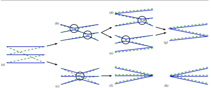
With the same approach they also considered the thermoelectric effect in ballistic Andreev interferometer [51],i.e.ballistic normal conducting regions coupled to two superconducting islands with a phase differenceφ. They considered different setups, with three of them shown in figure 8.1, with two of them being pretty much the same as for the conductance. For the first setup they found a vanishing thermopower due to the symmetry in φ caused by the symmetry in exchanging the leads. For the other setups they found a thermopower antisymmetric in the phase difference

The aim of this diploma thesis is to show that trajectory based semiclassics may be used to describe several properties of chaotic Andreev billiards. For that we start with reviewing the most important facts about Andreev billiards in section 2. These are the scattering formulation which connects the density of states to the scattering matrix of the normal region and the Landauer-type formulae for electronic and thermal transport. Then the semiclassical framework will be introduced starting from the path integral approach to quantum mechanics in section 3.1. In the same section this method is then used to derive the semiclassical Greens function in which is essentially given by the action of classical trajectories and their stability. Using this Greens function one also easily ﬁnds a semiclassical expression for the

(10)

4 Introduction T. Engl scattering matrix and therefore for the transmission coefficients. In section 4 we present the trajectory sets contributing in the semiclassical limit ~ →0 as well as some diagrammatic rules for these sets of trajectories. Having these diagrammatic rules we are then readily prepared to calculate the density of states of chaotic Andreev billiards in section 5 where we review the results for the density of states of Andreev billiards with just one superconducting lead presented in [48] and to extend the calculations to Andreev billiards with two superconducting leads with a phase differenceφin section 6. Additionally we take a brief look at the effect of small superconducting gaps. The dependence on an applied magnetic field and the effect of a non-zero Ehrenfest time is also taken into account. After that in section 7 we consider the transport properties of Andreev billiards consisting of two normal and two superconducting leads having the same chemical potential but different phases. We extend the work of [49] to all orders in N_S/N_N and show that the size of the superconductor plays an important role. Moreover we investigate the effect of a phase difference between two superconductors as well as the effect of an applied magnetic field and non-zero temperature. Finally in section 8 we apply the methods derived in section 7 to the thermopower for the first three setups of [51], i.e.the symmetric and asymmetric house as well as the parallelogram which consists of two dots connected by a neck and with each dot having one normal and one superconducting lead. We show that when going beyond the diagonal approximation a non-zero thermopower antisymmetric in the phase differenceφarises.

Please note that parts of this diploma thesis have already been submitted for publication [52] or are close to being published.

(11)

2 Theory of Andreev billiards

2.1 Scattering formulation of the density of states

2.1.1 Bogoliubov-De Gennes equation

The theory of Andreev billiards has been reviewed in detail by Beenakker in [25]. Here we will just repeat the most important facts. The electrons and holes of a closed normal metal-superconductor hybrid system are described by the Bogoliubov-de Gennes (BdG) equation [26]

HBG

( u v

)

=E ( u

v )

(2.1a) HBG=

( H ∆(r)

∆^∗(r) −H^∗ )

(2.1b) which is the analog to the ‘usual’ Schrödinger equation and is in principle a Schrödinger equation with a coupling between the electrons and holes. HereH = (p+eA)²/(2m) +V −EF is the Hamiltonian of an electron like quasiparticle and−H^∗ (the negative of the complex conjugated ofH) the Hamiltonian of a hole like quasiparticle. p = ∂/∂r = (∂/∂x, ∂/∂y, ∂/∂y)^T is the momentum operator where the superscript ‘T’ stands for transposed, A(r) the vector potential of an eventually applied magnetic field B,V(r) an arbitrary potential,e.g.an electrostatic potential, andE_F is the energy. Note that with this definition the energyEis measured with respect to the Fermi energy. u(r) andv(r) are electron and hole wave functions, respectively. The electron and hole wave functions are coupled by the superconducting pair potential ∆(r). One may easily prove that if (u, v)^T is an eigenvector with eigenvalueE, (−v^∗, u^∗)^T is also an eigenfunction with eigenvalue −E. Thus the complete set of eigenvalues lies symmetrically around zero.

At an interface between a normal metal and a superconductor the pairing interaction drops to zero over atomic distances at the normal region. Therefore we will use the step function model

∆(r) =

{ ∆e^iφ^j ifr∈S_j, j= 1,2

0 ifr∈N , (2.2)

where Sj stands for the j-th superconductor and N for the normal metal. This step function model is also known as the “rigid boundary condition” [53].

2.1.2 Excitation spectrum

Within the step function model the excitation spectrum of the coupled electron-hole quasiparticles can be expressed entirely in terms of the scattering matrix of the normal conducting region [54] which connects the outgoing waves to the incoming ones (see ﬁgure 2.1). Note that in order to get a well deﬁned scattering problem the interface between the normal region to the superconductors are assumed to be provided by ideal normal leads. Nevertheless we will call these leads as well as the channels they provide

‘superconducting’. Furthermore we assume that the only scattering process in the superconductor is pure Andreev reﬂection at the N-S interface. This also requires that the Fermi energyEFis much bigger than the superconducting bulk gap ∆.

One ﬁrst of all has to construct a basis for the scattering matrix which should be normalised to unit ﬂux. This may be achieved by writing the eigenfunctions of the BdG equation in the normal lead in the

(12)

6 Theory of Andreev billiards T. Engl

0000000 1111111

0000000 1111111 00000

00000 00000 00000 11111 11111 11111 11111

00000 00000 00000 00000 00000 11111 11111 11111 11111 11111

000000000000000000000000000000000 000000000000000000000000000000000 000000000000000000000000000000000 000000000000000000000000000000000 000000000000000000000000000000000 000000000000000000000000000000000 000000000000000000000000000000000 000000000000000000000000000000000 000000000000000000000000000000000 000000000000000000000000000000000 000000000000000000000000000000000 000000000000000000000000000000000 000000000000000000000000000000000 000000000000000000000000000000000 000000000000000000000000000000000 000000000000000000000000000000000 000000000000000000000000000000000 000000000000000000000000000000000 000000000000000000000000000000000 000000000000000000000000000000000 000000000000000000000000000000000 000000000000000000000000000000000 000000000000000000000000000000000

111111111111111111111111111111111 111111111111111111111111111111111 111111111111111111111111111111111 111111111111111111111111111111111 111111111111111111111111111111111 111111111111111111111111111111111 111111111111111111111111111111111 111111111111111111111111111111111 111111111111111111111111111111111 111111111111111111111111111111111 111111111111111111111111111111111 111111111111111111111111111111111 111111111111111111111111111111111 111111111111111111111111111111111 111111111111111111111111111111111 111111111111111111111111111111111 111111111111111111111111111111111 111111111111111111111111111111111 111111111111111111111111111111111 111111111111111111111111111111111 111111111111111111111111111111111 111111111111111111111111111111111 111111111111111111111111111111111

Lead 1

Lead 2 in₂ in₁

out₁

out₂

S( ) ε

Figure 2.1: The wave outgoing wave function which is given by a linear combination of the wave functions of the given channelsi= 1,2, . . .with coeﬃcients out1,i,out2,iis connected to the incoming wave function with coeﬃcients in1,i,in2,i by the scattering matrixS via (out1,out2)^T =S(in1,in2)^T.

form

Ψ^±_n,e(N) = ( 1

0 ) 1

√k_nêΦn(y, z)e^±îkêⁿ^x (2.3a) Ψ^±_n,h(N) =

( 0 1

) 1

√ k_n^h

Φ_n(y, z)e^±^ik^hⁿ^x, (2.3b)

where k_n^e,h = √ 2m(

E_F−E_n+σ^e,hE)

/~ and σ^e = 1, σ^h = −1. Furthermore the index n labels the modes which are equivalent to the channels, Φ_n(y, z) is the transverse wave function of the n-th mode normalised to unity andE_n is given by

[(p²_y+p²_z)

/(2m) +V(y, z)]

Φ_n(y, z) =E_nΦ_n(y, z).

Note that here the local coordinate system has been chosen such that the N-S interface is atx= 0.

Inside the superconductor Sj the eigenfunctions are given by Ψ^±_n,e(Sj) =

( eîηê^j^/2 e⁻îη^jê^/2

) 1

√2q^e_n

(E²/∆²−1)₋1/4

Φn(y, z)e^±^iq^eⁿ^x (2.4a) Ψ^±_n,h(Sj) =

( e^iη^h^j^/2 e⁻^iη^j^h^/2

)

√1 2q_n^h

(E²/∆²−1)₋1/4

Φn(y, z)e^±^iq^hⁿ^x (2.4b)

with

q^e,h_n =

√2m

~ [

EF−En+σ^e,h(

E²−∆²)1/2]1/2

(2.5a) η^e,h=φj+σ^e,harccos

(E

∆ )

. (2.5b)

The wave functions (2.3a,b) and (2.4a,b) are normalised to carry the same amount of quasiparticle current.

This in turn ensures the unitarity of the scattering matrix. The direction of the velocity is the same as the wave vector for the electron and opposite for the hole.

A wave incident on the Andreev billiard is described in the basis (2.3a,b) by a vector of coeﬃcients cⁱⁿ_N =(

c⁺_e, c⁻_h)

while the reflected wave has a vector of coefficientscôut_N =( c⁻_e, c⁺_h)

. The N here refers to the fact that the waves are in the normal lead. The mode indexnhas been dropped here for simplicity of notation. The scattering matrix of the normal conducting region connects these two waves to each other

(13)

T. Engl Semiclassics of Andreev billiards 7 viac^out_N =SNcⁱⁿ_N. Since the normal conducting region does not couple electrons and holes its scattering matrix has the block diagonal form

S_N(E) =

( S(E) 0 0 S(−E)^∗

)

. (2.6)

Here S(E) is the N ×N unitary scattering matrix of the normal region itself corresponding to the single-electron HamiltonianH.

For energies 0< E <∆ there are no propagating modes in the superconducting lead and the scattering matrixSA of Andreev reflection at the N-S interface can be defined bycⁱⁿ =SAcôut. Its elements can be obtained by matching the wave functions in (2.3a,b) to the corresponding ones in (2.4a,b) at x= 0.

Note that we also assume thatEF∆ such that normal reflection at the N-S interface may be ignored and the difference in the numbers of channels for positive and negative energies may be neglected. This is known as the Andreev approximation [27]. The entries of the scattering matrix of Andreev reflection are therefore given by

SA(E) =α(E) (

0 e^{i ˜}^φ e⁻^{i ˜}^φ 0

)

, (2.7)

where α= e⁻i arccos(E/∆) =E/∆−i√

1−E²/∆² and ˜φ is a diagonal matrix with its ﬁrstNS₁ entries equal toφ1, the nextNS₂ entries equal toφ2etc. whereNS_j,j ∈ {1, . . . , n}, is the number of channels of thej-th superconducting lead,nthe number of superconducting leads andφj,j ∈ {1, . . . , n}, the phase of thej-th superconductor.

As already mentioned below, ∆ there are no propagating modes in the superconductor. Therefore the bound states require thatcin=SASNcin. Thus we have to solve an eigenvalue problem, and the bound states are given by det (1−SASN) = 0. When insertingSAandSN and using

det

( A B C D

)

= det(

AD−ACA⁻¹B)

(2.8) for arbitrary matrices A, B, C and D, the discrete spectrum below ∆ is given by the determinental equation [54]

det [

1−α(E)²e⁻^{i ˜}^φS(E)e^{i ˜}^φS(−E)^∗ ]

= 0. (2.9)

2.1.3 Density of states

In mesoscopic systems, where the density of states is big, one can no longer talk about single Andreev lev- els. Furthermore one has to investigate averaged quantities. An equation giving the averaged density of states directly may be found starting with (2.9) by a similar calculation as done in [55]. The scattering matrix in the secular function therein has to be replaced by the product ¯S(E) =−α(E)²e⁻^{i ˜}^φS(E)e^{i ˜}^φS(−E)^∗ thus giving a modiﬁed secular function

Z_sc⁰ (E) = det[

1 + ¯S(E)]

. (2.10)

S(E) is obviously unitary below ∆. Therefore its eigenvalues lie on the unit circle of the complex plane¯ and may be written as e^iθⁿ^(E)withn= 0, . . . ,2NS. The phasesθn(E) are the eigenphases of the scattering matrix. Therefore we can express the modiﬁed secular function in terms of the eigenphasesθn(E) of ¯S(E),

Z_sc⁰ (E) =

NS

∏

n=1

(

1 + e^iθⁿ^(E) )

= exp (

i

NS

∑

n=1

θn(E) 2

) 2^N^S

NS

∏

n=1

cos

(θn(E) 2

)

. (2.11)

In the second step a factor e^iθⁿ^(E)/2 has been extracted out of each term in the product such that the remaining terms are equal to 2 cos(θ_n(E)/2). The real valued zeros which account for the spectrum

(14)

8 Theory of Andreev billiards T. Engl provide the factors cos(θn(E)/2). Hence the number of eigenenergies in the interval (0, E) is given by (see Appendix B for a reasoning)

N(E) =−1 π lim

ε→0Im ln

NS

∏

n=1

cos

(θ_n(E+ iε) 2

)

= 1 2π

NS

∑

n=1

θn(E)−1 π lim

ε→0Im ln ¯S(E+ iε). (2.12) In the following we will drop theεalthough it will always be implicitly present. The density of states is then obtained by diﬀerentiating (2.12) with respect to the energy.

d(E) = ¯˜ d(E)− 1 πIm ∂

∂Eln det [

1−α(E)²e⁻^{i ˜}^φS(E)e^{i ˜}^φS(−E)^∗ ]

. (2.13)

Here ¯d(E) is twice the mean density of states. The logarithm of a determinant of a matrix can be written as the trace of the logarithm of the matrix deﬁned by its Taylor series which we will use to derive the density of states in terms of traces of powers of the scattering matrix. We now divide by d(E) =¯ N/(2πET) and express the energy in units of the Thouless Energy=E/ET, whereET= 2~/τD

andτDis the mean dwell time, which is the time a quasiparticle stays on average inside the cavity between two succeeding Andreev reﬂections. The density of states in terms of then reads ifφ1, . . . , φk are the phases of the superconducting order parameters in thek leads

d() = 1 + 2

∑∞ n=1

α²ⁿ

n Im∂C(, n, φ1, . . . , φk)

∂ (2.14)

with the correlation functions of n scattering matrices multiplied by a diagonal matrix containing the phases of the superconductors.

C(, n, φ₁, . . . , φ_k) = 1 NTr

[ e⁻^{i ˜}^φS^∗

(

− ~ 2τ_D

) e^{i ˜}^φS

( ~ 2τ_D

)]n

. (2.15)

From now on we will restrict ourselves to Andreev billiards with two superconductors with phasesφ₁and φ2, respectively. Then the correlation function and the density of states of course will only depend on the diﬀerence φ=φ1−φ2 such that we will call the correlation function in this caseC(, n, φ) and in the case that there is just one superconductor the phase should not play any role so that we will write C(, n).

2.2 Random matrices versus diagonal approximation

2.2.1 Random matrix theory

Equation (2.9) is the starting equation for the calculation of the density of states when using Random matrix theory (RMT). In RMT the Hamiltonian of the system is replaced by matrices with randomly chosen entries following a certain distribution. In the end one averages over many of these randomly chosen matrices. It is believed that a quantum system which underlying classical dynamic is chaotic is well described by RMT [56]. This is the Bohigas-Gianonni-Schmidt- (BGS-) conjecture.

The RMT approach to the density of states of an chaotic Andreev billiard was initially considered in [33, 41] where the actual setup treated is depicted in ﬁgure 2.2. It consists of a normal metal (N) connected to two superconductors (S₁, S₂) by narrow leads carryingN_S₁ andN_S₂ channels. The superconductors’

order parameters are considered to have phases ±φ/2, with a total phase difference φ. Moreover a perpendicular magnetic fieldB was applied to the normal part. We note that although this figure have spatial symmetry the treatment is actually for the case without such symmetry.

As above, the limit ∆E_Fwas taken so that normal reﬂection at the N-S interface can be neglected and the symmetric case where both leads contain the same number, N_S/2, of channels was considered

(15)

T. Engl Semiclassics of Andreev billiards 9

N_S

1 N_S

2

N_S

B

S₁ S₂

−__

2 __ φ

+ 2 φ

Figure 2.2: An Andreev billiard connected to two superconductors (S₁, S₂) at phases ±φ/2 via leads carryingN_S₁ andN_S₂ channels, all threaded by a perpendicular magnetic ﬁeldB.

[33, 41]. Finally it was also assumed thatα≈ −i, valid in the limitE, ET∆EF. For such a setup, the determinantal equation (2.9) becomes

det [

1 +S(E)e^{i ˜}^φS^∗(−E)e⁻^{i ˜}^φ ]

= 0, (2.16)

where ˜φis a diagonal matrix whose ﬁrstNS/2 elements areφ/2 and the remainingNS/2 elements−φ/2.

We note that though we stick to the case of perfect coupling here, the eﬀect of tunnel barriers was also included in [33].

The ﬁrst step is to rewrite the scattering problem in terms of a low energy eﬀective HamiltonianH H=

( Hˆ πXX^T

−πXX^T −Hˆ^∗ )

, (2.17)

where ˆH is theM×M Hamiltonian of the isolated billiard andX anM×N coupling matrix. Eventually the limitM → ∞is taken and to mimic a chaotic system the matrix ˆH is replaced by a random matrix following the Pandey-Mehta distribution [57]

P(H)∝exp



−N_S²( 1 +a²) 64M E_T²

∑M i,j=1

[(

Re ˆH_ij )2

+a⁻² (

Im ˆH_ij )2]

. (2.18)

The parameterameasures the strength of the time-reversal symmetry breaking so we can investigate the crossover from the ensemble with time reversal symmetry (GOE) to that without (GUE). It is related to the magnetic ﬂux Φ through the two-dimensional billiard of area A and with Fermi velocityvFby

M a²=c (eΦ

h )2

~vF

N 2πE_T√

A. (2.19)

Here c is a numerical constant of order unity depending only on the shape of the billiard. The critical ﬂux is then deﬁned via

M a²= N 8

(Φ Φ_c

)2

⇔ Φ_c≈ h e

(2πET

~v_F )¹₂

A¹⁴. (2.20)

The density of states, divided for convenience by twice the mean density of states of the isolated billiard, can be written as

d() =−ImW(), (2.21)

(16)

10 Theory of Andreev billiards T. Engl

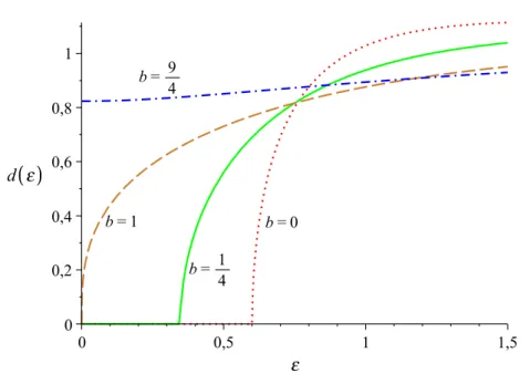
Figure 2.3: The density of states obtained using RMT (solid) and the diagonal approximation (dashed).

While RMT predicts an hard gap up to ≈ 0.6ET the Bohr-Sommerfeld result is just exponentially suppressed.

where W() is the trace of a block of the Green function of the eﬀective Hamiltonian of the scattering system and for simplicity here we express the energy in units of the Thouless energy=E/ET. This is averaged by integrating over (2.18) using diagrammatic methods [58], which to leading order in inverse channel number 1/NSleads to the expression [41]

W() = (b

2W()− 2

) (

1 +W²() +

√1 +W²() β

)

, (2.22)

whereβ= cos (φ/2) andb= (Φ/Φc)²with the critical magnetic flux Φc for which the gap in the density of states closes (atφ= 0). Equation (2.22) may also be rewritten as a sixth order polynomial and when substituting into (2.21), we should take the solution that tends to 1 for large energies. In particular, when there is no phase difference between the two leads (φ= 0, or equivalently when we consider a single lead carryingN_Schannels) and no magnetic field in the cavity (Φ/Φ_c = 0) the density of states is given by a solution of the cubic equation

²W³() + 4W²() + (4 +²)W() + 4= 0. (2.23)

2.2.2 Diagonal approximation

The diagonal approximation will be introduced in section 4.1 but we anticipate the result obtained previously when using the diagonal approximation for the density of states of Andreev billiards without going into the details at this stage. In [36] the authors found a density of states of an Andreev billiard with just one superconducting lead given by

d_BS() = (π

)2 cosh(π/)

sinh²(π/). (2.24)

The results of the RMT prediction given by the solution of (2.23) and the Bohr-Sommerfeld result (2.24) are compared to each other in ﬁgure 2.3. The density of states predicted by RMT for one superconducting lead and zero magnetic ﬁeld is compared to the prediction of the semiclassical calculation based on the

(17)

T. Engl Semiclassics of Andreev billiards 11

0000000 1111111

0000000 1111111 00000

00000 00000 00000 11111 11111 11111 11111

00000 00000 00000 00000 00000 11111 11111 11111 11111 11111

Lead 1

Lead 2 T1

N1 T₂

N₂

11 T

T T

αβ21

12αβ αβ

α β

αβ

α β

Figure 2.4: Three examples for paths contributing to the transmission from lead 1 to lead 2T₂₁^αβ, from lead 1 back to lead 1T₁₁^αβand from lead 2 to lead 1T₁₂^αβwhile being converted from aβ-type quasiparticle to anα-type one. The leads provideN₁ andN₂channels respectively and have temperaturesT₁ andT₂.

diagonal approximation. While the density of states has a hard gap of the order of the Thouless energy, i.ethat it is zero up to an energy≈0.6E_T, the Bohr-Sommerfeld result is only exponentially suppressed for low energies. We will see in section 5 how this discrepancy may be resolved.

2.3 Transport theory

Another problem often considered in condensed matter physics, but also closely related to the scattering matrix is electrical transport. For this we attach additional normal leads to the normal region.

The transport through N-S junctions as well as the theory of the transport through a phase coherent superconductor-normal metal hybrid systems has been reviewed in [59]. Originally the theory we will use here was developed by Lambert [60] for a two terminal system and was later generalised to multi- probe systems [61]. It yields a variety of transport coefficients including electrical transport and was derived under the condition that the condensate chemical potentialsµ of all superconducting leads are identical. This condition allows one to consider time independent order parameter phases and a time independent scattering approach is applicable. Lambert’s derivation of the fundamental current-voltage relation is fairly similar to the multi-channel scattering theory developed by Landauer and Büttiker [29] for non-superconducting mesoscopic structures. In this approach which is now well known as the Landauer-Büttiker formalism, the electrical conductanceG_ij for a current from leadj to leadiof a two terminal device is related to the transmission coefficientT_ijêeof an electron entering the scattering region at leadj and leaving it at leadias an electron as shown in figure 2.4 with choosingα=β=e,

Gij= e²

π~T_ij^ee, (2.25)

where ~ is Planck’s constant and the superscript ee here denotes that the incoming and outgoing quasiparticle are both electrons. We will always make use of~rather than ofh= 2π~, although usually in the literature h is used, in order to avoid mixing it up with the ‘h’ used for labeling holes. This however is not valid in the presence of Andreev scattering since for example this process separates charge and energy: If a quasiparticle hits the interface and is Andreev reﬂected the energy of the excitation is reﬂected back into the superconductor while a charge of 2e is injected into the superconductor (c.f. [59]).

2.3.1 Conductance of a multi-probe structure

It is no longer enough to consider the scattering matrix of the normal conducting region as done for the density of states. Instead one has to make use of a more general scattering matrix which also allows conversions from an electron-like to hole-like quasi particle or vice versa. This generalised scattering

(18)

12 Theory of Andreev billiards T. Engl matrix ˜S(E) may be written in four blocks

S(E) =˜

( S^ee(E) S^eh(E) S^he(E) S^hh(E)

)

, (2.26)

whereS^αβ(E) is the scattering matrix which connects the coefficients of the outgoing wave functions of aβ type quasiparticle to the coefficients of the incoming wave functions of anαtype quasiparticle. Note that this is just one possibility to write this generalised scattering matrix. The block form used here holds if the vector of incoming and outgoing wave coefficients is filled by the coefficients of the electron wave functions before the first coefficient of a hole wave function is entered. A different form has been used in [59, 60] where the authors used the two component wave function such that the wave functions have two components. The generalised scattering matrix has all the known properties of the scattering matrix of the normal metal with all their consequences: It is unitary ensuring current conservation and if an applied magnetic field is reversed this is equivalent to transposing the generalised scattering matrix.

Moreover, if the energy E is measured with respect to the condensate chemical potential µ, it satisﬁes the electron hole symmetry relationS^αβ(E) =−(−1)^δ^αβ[S^α^¯^β^¯(−E)]^∗, where ¯αdenotes a hole ifαdenotes an electron and vice versa.

The coeﬃcientsT_kl^αβ(E) for the transmission of aβtype quasiparticle in leadlto anαtype quasiparticle in leadkas those depicted in ﬁgure 2.4 is given by the entries ofS^αβ(E) via

T_kl^αβ(E) =∑

o,i

S_oi^αβ(E)², (2.27)

where the sum runs over all channels o in lead k (we will refer to it as an ‘outgoing’ channel) and all channels i in lead l (we will refer to it as an ‘incoming’ channel). The properties of the generalised scattering matrix imply some important properties of the transmission coeﬃcients. These are

∑

β,l

T_kl^αβ(E) =∑

α,l

T_kl^αβ(E) =Nk (2.28)

due to the unitarity of ˜S(E), particle-hole symmetry

T_kl^αβ(E) =T_kl^α^¯^β^¯(−E) (2.29) and the time reversibility saying that when reversing an applied ﬁeld this is equivalent to exchangingk andlas well asαandβ. Note that for simplicity of notation we have assumed that the number of open channels in each lead is equal for electrons and holes.

Analogously to the Landauer-B¨uttiker formalism [29] the current in leadkis given by Ik= e

π~

N_N

∑

j=1

∑

α=e,h

σ^α

∫∞ 0

dE



δ_klNkf_k^α(E)− ∑

β=e,h

T_kl^αβ(E)f_l^β(E)



, (2.30)

where f_l^α(E) = exp{−[E−σ^α(eV_l−µ)]/(k_BT)} is the Fermi function for an αtype quasiparticle, V_l is the voltage applied to the l-th lead and N_N is the total number of channels of all the normal leads together. The typical Landauer-Büttiker formula is derived in the linear response regime. This is that the voltage differences are small such that the occurring Fermi functions can be expanded around the chemical potential of the superconductors up to first order in the voltage differences. If we do so apart from different signs the Fermi functions for electrons and holes will be the same and the entries of the conductance matrix which entries connect the current in the k-th lead to the voltages in the different leads viaIk =∑

lGkl(Vl−VS) withVS=µ/e are G_kl= e²

π~

∫∞ 0

d[

2δ_klN_k−T_kl^ee() +T_kl^eh()−T_kl^hh() +T_kl^he()] (

−∂f()

∂ )

, (2.31)

(19)

T. Engl Semiclassics of Andreev billiards 13 where the energy is again measured in units of the Thouless energyET. If one applies the electron-hole symmetry (2.29) one could remove for example T_kl^hh() and T_kl^he() in (2.31) by extending the integral over the energy to−∞.

2.3.2 Two-probe formulae

In the case of two normal leads the current-voltage relation may be written in matrix form ( I₁

I₂ )

=

( G₁₁ G₁₂ G₂₁ G₂₂

) ( V₁−V_S V₂−V_S

)

. (2.32)

The conductance matrix connecting the current to the applied voltages is then given by ( G11 G12

G21 G22

)

= e² π~

∫∞

−∞

d

( N1−T₁₁êe() +T₁₁^he() T₁₂^he()−T₁₂êe() T₂₁^he()−T₂₁êe() N2−T₂₂êe() +T₂₂^he()

) (

−∂f

∂ )

. (2.33) Note that we have used the electron hole symmetry to extend the integral to−∞.

If the superconducting condensate chemical potential is not controlled externally it adjusts itself so that the net current through the N-S interfaces are zero and therefore the current in lead 2 has to be the opposite of that in lead 1,i.e. I₁=−I₂=I. The conductanceGof the system may then be calculated byG=I/(V₁−V₂). For this we ﬁrst have to eliminate the chemical potential of the superconductors.

Thus one ﬁrst has to invert (2.32) giving ( V1−VS

V2−VS

)

= 1 d

( G22 −G12

−G21 G11

) ( I

−I )

(2.34) with the determinant of the conductance matrixd=G11G22−G12G21. At zero temperature the derivative of the Fermi function becomes aδ-function and all the transmission and reﬂection coeﬃcient have to be evaluated at= 0 and the dimensionless conductance g=Gπ~/e² which measures the conductance in units of the conductance quantum e²/π~therefore reads [61]

g=T₂₁^ee+T₂₁^he+ 2(

T₁₁^heT₂₂^he−T₂₁^heT₁₂^he)

T₁₁^he+T₂₂^he+T₂₁^he+T₁₂^he. (2.35) In this equation the number of channelsNihas been replaced by transmission coeﬃcients by using (2.28).

For a symmetric scatterer, where T₁₂^αβ =T₂₁^αβ and T₂₂^αβ = T₁₁^αβ this reduces to g = T₂₁êe+T₁₁^he whereas in absence of transmission between the two leads the resistanceg⁻¹ reduces to a sum of two resistances g⁻¹ = (2T₁₁^he)⁻¹+ (2T₂₂^he)⁻¹. When combining the particle hole symmetry with the unitarity of the scattering matrix one finds thatT₂₁êe+T₂₁^he=T₁₂êe+T₁₂^heand thus (2.35) is symmetric under exchanging primed and unprimed coefficients.

2.4 Thermopower

If the different leads have, additional to the different voltagesV_j, different temperaturesT_j then equation (2.30) has to be slightly modified. Each transmission (and reflection) coefficient T_kl is multiplied with the Fermi function of the incoming leadl [62] and hence depends on the temperature T_l of this lead, i.e.the Fermi functions in (2.30) are now given by f_l^α(E) = exp{−[E−α(eVl−µ)]/(kBTl)}, where Tl is the temperature in thel-th lead. With this replacement (2.30) also describes the thermoelectrical effect,i.e.that a temperature difference causes a voltage difference.

If one again linearises (2.30) with the Fermi functions with diﬀerent temperatures not only in the voltage but also in the temperatures one ﬁnds for a two terminal setup with isolated superconducting leads, where the net electrical current and heat current in the superconducting leads are zero [63]

( I1

I₂ )

=G

( V1−VS

V₂−V_S )

+B

( T1−T T₂−T

)

, (2.36)