Algorithms for streaming graphs

(1)

Algorithms for Streaming Graphs

DISSERTATION

zur Erlangung des akademischen Grades doctor rerum naturalium

(Dr. rer. nat.) im Fach Informatik

eingereicht an der

Mathematisch-Naturwissenschaftlichen Fakultät II Humboldt-Universität zu Berlin

von

Herr Dipl.-Inf. Mariano Zelke

geboren am 12.11.1978 in Lutherstadt Wittenberg

Präsident der Humboldt-Universität zu Berlin:

Prof. Dr. Dr. h.c. Christoph Markschies

Dekan der Mathematisch-Naturwissenschaftlichen Fakultät II:

Prof. Dr. Wolfgang Coy Gutachter:

1. Prof. Dr. Martin Grohe 2. Prof. Dr. Stefan Hougardy 3. Prof. Dr. Ulrich Meyer

eingereicht am: 13.11.2008

Tag der mündlichen Prüfung: 18.02.2009

(2)

(3)

Abstract

An algorithm solving a graph problem is usually expected to have fast random access to the input graph G and a working memory that is able to storeGcompletely. These powerful assumptions are put in question by massive graphs that exceed common working memories and that can only be stored on disks or even tapes. Here, random access is very time-consuming.

To tackle massive graphs stored on external memories, Muthukrishnan proposed the semi-streaming model in 2003. It permits a working memory of restricted size and forbids random access to the input graph. In contrast, the input is assumed to be a stream of edges in arbitrary order.

In this thesis we develop algorithms in the semi-streaming model approaching different graph problems. For the problems of testing graph connectivity and bipartiteness and for the computation of a minimum spanning tree, we show how to obtain running times that are asymptotically optimal.

For the problem of finding a maximum weighted matching, which is known to be intractable in the semi-streaming model, we present the best known approximation algorithm. Finally, we show the minimum and the maximum cut problem in a graph both to be intractable in the semi-streaming model and give semi-streaming algorithms that approximate respective solutions in a randomized fashion.

Keywords:

streaming algorithm, graph, minimum spanning tree, matching

(4)

(5)

Zusammenfassung

Für einen Algorithmus zum Lösen eines Graphenproblems wird üblicherwei- se angenommen, dieser sei mit wahlfreiem Zugriff (random access) auf den Eingabegraphen G ausgestattet, als auch mit einem Arbeitsspeicher, der G vollständig aufzunehmen vermag. Diese Annahmen erweisen sich als frag- würdig, wenn Graphen betrachtet werden, deren Größe jene konventioneller Arbeitsspeicher übersteigt. Solche Graphen können nur auf externen Spei- chern wie Festplatten oder Magnetbändern vorrätig gehalten werden, auf denen wahlfreier Zugriff sehr zeitaufwändig ist.

Um riesige Graphen zu bearbeiten, die auf externen Speichern liegen, hat Muthukrishnan 2003 das Modell eines Semi-Streaming Algorithmus vorge- schlagen. Dieses Modell beschränkt die Größe des Arbeitsspeichers und ver- bietet den wahlfreien Zugriff auf den Eingabegraphen G. Im Gegenteil wird angenommen, die Eingabe sei ein Datenstrom bestehend aus Kanten von G in beliebiger Reihenfolge.

In der vorliegenden Dissertation entwickeln wir Algorithmen im Semi- Streaming Modell für verschiedene Graphenprobleme. Für das Testen des Zusammenhangs und der Bipartität eines Graphen, als auch für die Berech- nung eines minimal spannenden Baumes stellen wir Algorithmen vor, die asymptotisch optimale Laufzeiten erreichen. Es ist bekannt, dass kein Semi- Streaming Algorithmus existieren kann, der ein größtes gewichtetes Matching in einem Graphen findet. Für dieses Problem geben wir den besten bekann- ten Approximationsalgorithmus an. Schließlich zeigen wir, dass sowohl ein minimaler als auch ein maximaler Schnitt in einem Graphen nicht von einem Semi-Streaming Algorithmus berechnet werden kann. Für beide Proble- me stellen wir randomisierte Approximationsalgorithmen im Semi-Streaming Modell vor.

Schlagwörter:

Datenstrom-Algorithmus, Graph, Minimal Spannender Baum, Matching

(6)

(7)

to my wife

(8)

(9)

Chapter 1 Introduction

“He had long ago concluded that he possessed only one small and finite brain, and he had fixed a habit of determining most carefully with what he would fill it.“

Annie Dillard, The Living Today‘s computational tasks are facing an increasing amount of data. Ocea- nographic and atmospheric information is processed for climate prediction; IP traffic data is analyzed for billing purposes and to maintain network services.

The volume of such massive data easily reaches terabytes or even petabytes.

The particle physics experiment at the large hadron collider of CERN [CER]

will soon produce data of a size of 15 petabytes per year [LHC] corresponding to more than 28 gigabytes on average every minute. That data is partly inspected in real-time but is also stored for later investigation.

In the traditional RAM model, c.f. [AHU75], an algorithm is assumed to be equipped with a memory that includes the whole input and allows fast random access to it. Every data item is within reach in no time at all.

These powerful assumptions are unreasonable for computational tasks as the above ones. Massive input data goes beyond the bounds of common main memories; thus, it is stored on disks or even tapes. Seek times, that is, movements of read/write heads are now dominating the time to call up single data items, making random access impractical. Moreover, if observed phenomena must be considered in a real-time manner, there is no random access at all.

(12)

This is where streaming algorithms arrive on the scene. They drop the requirement of random access to the input. By contrast, the input is assumed to arrive in arbitrary order as an input stream. In addition, the working memory of a streaming algorithm is constrained to be small compared to the size of the input; hence, it does not allow to memorize the whole input stream.

Streaming algorithms are not only useful to process arising data in real- time without completely storing it. Moreover, they provide a reasonable framework for processing data that is stored on external memory devices. For developing time-efficient algorithms working on these storage components, it is reasonable to assume the input of the algorithm (which is the output of the storage device) to be a sequential stream. While tapes produce a stream as their natural output, the output rate of a disk drastically grows if its content is accessed sequentially in the order it is stored.

Apart from their usefulness in practice, streaming algorithms also provide new insights into computational problems. While there is a developed theory for algorithms with bounded working memory, see e.g. [Pap94], com- paratively few is known about the combination of bounded memory with forbidden random access. Such new insights may change the way we tackle computational tasks even for small problem instances. As it turns out in Chapter 4, there are problems that can be approached by a streaming algorithm within the same time bounds as in the RAM model. As a result, the transfer of the problem instance from an external memory into the main memory before starting the computation can be omitted. Instead, the computation can take place while the instance is read from the external device.

Most of the previous work in the area of data stream algorithms is focused on streams comprising numerical values. On such streams statistical data like norms [Ind06], histograms [GGI⁺02], and quantiles [CKMS06] are of interest as well as the most frequent items [MAA06]. A comprehensive overview on the field of numerical streams is given by Babcock et al. [BBD⁺02] and Muthukrishnan [Mut05].

However, plenty of the emerging data can be regarded as a graph. The call graph of AT&T, modeling the users as vertices and the telephone calls as edges between them, consists of 200 million edges for every single day [Par08].

Not only for troubleshooting and forecasting, structural knowledge of this graph is of great interest. It can also help to identify fraudulent behav- ior [CPV02].

An even bigger graph is the web graph whose vertices are the webpages, two of them joined by a directed edge if there is a hyperlink in between. The

(13)

3

discovery of structural information about this graph is a streaming problem:

Since there is no explicit storage of the web graph, there is no random access to it. Instead, vertices and edges are spotted by web crawlers, i.e, little software agents that move along hyperlinks and report them to a server.

There are approaches to reveal the topology of the web graph [BAJ00] or to utilize the connectivity structure to detect emerging communities [KRRT99].

To handle graph issues in a streaming context, Muthukrishnan [Mut05]

proposed thesemi-streaming model: The input graph is presented as a stream of its edges in arbitrary order to a semi-streaming algorithm. The working memory of this algorithm is restricted to allow the storage of all vertices but only a polylogarithmic number of edges on average for every vertex.

Hence, input graphs that are too dense cannot be stored completely within the working memory. To find space-efficient summarizations for such graphs according to the query to be answered, is the challenge for a semi-streaming algorithm.

This thesis is concerned with semi-streaming algorithms tackling different graph problems. Chapter 2 formally introduces the semi-streaming model and its parameters while Chapter 3 summarizes related work in the area of graph problems under streaming assumptions. Chapter 4 presents the results obtained in [Zel07] about optimal processing times for some basic problems on graphs and slightly extends these results for k-vertex and k- edge connectivity. The problem of finding a maximum weighted matching is the focus of Chapter 5 that covers results of [Zel08]. Chapter 6 investigates the possibilities to find minimum and maximum cuts in graphs. A conclusion of the whole thesis can be found in Chapter 7.

Each of Chapters 4-6 starts with an introductory section giving the neces- sary definitions as well as the related work and contains concluding remarks at its end. Provided the reader is familiar with the basic concepts of graph theory, cf. [Die05], and the formal definition of the semi-streaming model, cf.

Chapter 2, every chapter is self-contained and should be coherent on its own.

(14)

(15)

Chapter 2 The Semi-Streaming Model

The semi-streaming model was coined by Muthukrishnan in 2003 [Mut05] to approach graph problems in the context of streaming.

Let G = (V, E) be a graph on the vertex set V and the edge set E.

We denote by n = |V| and m = |E| the number of vertices and edges, respectively. A sequence of the edges of G in arbitrary order we call agraph stream. Asemi-streaming algorithm is presented a graph stream of Gas the input. The algorithm’s working memory is restricted toO(n·polylogn) bits, where polylogn denotes log^sn for some constants.

A semi-streaming algorithm may access the graph stream for P passes.

Each pass starts at the beginning of the stream and goes over it in the same sequential one-way order. For all algorithms developed in this thesis, we haveP = 1, that is, we are only concerned with algorithms that are content with a single pass over the input stream.

A key parameter of a semi-streaming algorithm is the per-edge processing timeT. We define this to be the minimum time allowed between the revealing of two consecutive edges in the input stream. This definition of T renders the definitions of early papers more precisely; we give a discussion concerning that in Section 2.1.

After reading the whole graph stream, the algorithm might spend some time on postprocessing before giving an output. This postprocessing time is incorporated by the computing time which is defined as the total time from reading the first edge in the graph stream until the answer of the algorithm is computed.

Note that the space restriction of the model allows the storage of a polylog-

(16)

arithmic number of edges on average for every vertex. Hence, a graph with O(n·polylogn) edges can be read entirely into the memory and treated in the postprocessing step. Such graphs are of no interest in this model since the intrinsic task for a streaming algorithm, that is, to make a space-efficient summarization of the input, becomes irrelevant. As a result, we will restrict our attention to graphs with ω(n·polylogn) edges.

2.1 Discussion on the Per-Edge Processing Time

Early papers about semi-streaming algorithms that consider the per-edge processing timeT [FKM⁺05b; FKM⁺05a; Zel06] useT in an ambiguous way.

While being used as the worst-case time to process a single edge on the one hand, it is equally used on the other hand, even if not explicitly stated, as amortized time charged over the number of edges. In fact, if tools as dynamic trees or disjoint set data structures are utilized, they give rise to amortized times since their time bounds are of amortized type as well. Processing the input edges is then assumed to be evenly spread over the whole computing time which is then assumed to be justm·T.

This definition is not appropriate for a streaming algorithm: As pointed out by Muthukrishnan [Mut05] the computing time, i.e., the time to evaluate the property in question for items read in so far, is not the most important parameter of a streaming algorithm. What is more crucial is the maximum frequency of incoming items that can still be considered by the algorithm.

That refers to the speed at which external storage devices can present their data content to a streaming algorithm and constitutes the frequency at which observed phenomena can be taken into account. To this aim it is desirable to maximize the potential rate of incoming items by postponing as much operations as possible to a moment after reading all input items, even at the cost of a higher computing time.

To model this worthwhile property of a streaming algorithm, we propose the definition of the per-edge processing timeT to be the minimum allowable time between two consecutive edges in the graph stream. Note that, on the one hand, this notion is weaker than the idea of a worst-case time: It might be the case that on several edges in the input stream the algorithm has to spend a time longer than T, that is, the worst case time might be higher.

But then edges arriving with a delay ofT can be buffered while the algorithm processes a time-consuming edge.

(17)

2.1. Discussion on the Per-Edge Processing Time 7 On the other hand, such a buffer can only carry O(n·polylogn) edges and must be flushed regularly. Therefore, our definition ofT is stronger than the notion of amortized time: The amortized notion allows the existence of edges whose processing is so time-consuming that succeeding edges overrun the buffer and cannot be considered by the algorithm. In contrast, our definition of T makes sure that a semi-streaming algorithm with that per-edge processing time is able to consider every single edge in a stream of edges arriving with a delay of T.

(18)

(19)

Chapter 3 Related Work

Since the work of Munro and Paterson [MP78] the area of streaming algorithms has become voluminous. In this chapter we give account to the work that has been done on graph problems in this area, i.e., where the input is composed of a graph’s edges and the memory is too small to carry all of them. For a comprehensive overview on the other aspects in the area of streaming not considering graph problems, we again refer the reader to the surveys of Babcock et al. [BBD⁺02] and Muthukrishnan [Mut05] and the rich bibliography therein.

The paper of Henzinger et al. [HRR99] is the first one to examine graph problems in the context of streaming. In this paper it is proven that to test the k-vertex and k-edge connectivity for 1 ≤ k < n and the planarity of a graph in P passes over the input requires Ω(n/P) bits of working memory.

The same lower bound is presented for the problem of finding all the sinks of a directed graph together with an algorithm for it that achieves the lower bound. Moreover, it is shown that to estimate the number of edges in the transitive closure of a directed graph to within any constant factor in one pass requires a working memory of Ω(m) bits.

An early natural streaming algorithm covering a graph problem is given by Bar-Yossef et al. [BYKS02] approximating the number of triangles in a graph. The algorithm works in a randomized fashion and its space usage depends on the desired approximation ratio and success probability as well as on the number of triangles and vertices in the input graph. The space consumption for solving this problem is improved by Jowhari and Ghodsi [JG05]

and further by Buriol et al. [BFL⁺06] where the dependency on the number of vertices is removed.

(20)

A paper of Buchsbaum et al. [BGW03] examines lower bounds for the problem of finding a pair of vertices that share a large common neighborhood.

In particular, it is shown that any one-pass algorithm that is able to decide the existence of a vertex pair with a common neighborhood of size 1< s < n requires Ω(n²) bits of working memory in the worst case. This bound holds for deterministic as well as for randomized algorithms.

Ganguly and Saha [GS06] study the complexity to compute P_k, that is, the number of vertex pairs that are connected via a path of length k. It is shown that findingP_k in one pass over the input requires a memory of Ω(n²) bits for any k ≥ 3. A randomized algorithm with a memory consumption ofO(logn·m(m−r)^1/4) bits that estimatesP₂ in a graph with r connected components is complemented with a lower bound of Ω(√

m) bits for that problem.

A formal motivation to extend the bound of o(n) bits of memory when considering graph problems in the streaming context is given by Feigenbaum et al. [FKM⁺05a]: A large class of graph properties called balanced properties is identified whose determination in one pass requires Ω(n) space. Many basic properties as connectivity, bipartiteness, and the existence of a vertex with a certain degree fall into this class.

Muthukrishnan [Mut05] anticipates the leap over the o(n) bit barrier when identifying a space restriction of O(n·polylogn) bits as the sweet spot for streaming algorithms tackling graph problems. He suggests the corresponding semi-streaming model as defined in Chapter 2 and initiates the search for semi-streaming algorithms approaching different problems.

Two papers of Feigenbaum et al. [FKM⁺05b; FKM⁺05a] consider some basic problems in the semi-streaming model. Algorithms using one pass over the input are given to compute the connected components and a bipartition of a graph with a per-edge processing time of T =O(α(n)) and a minimum spanning forest with T = O(logn). Here, α(n) denotes a natural inverse of Ackermann’s function defined in Chapter 4. Moreover, [FKM⁺05b;

FKM⁺05a] present algorithms testing a graph’sk-vertex connectivity fork ≤ 4 and its k-edge connectivity for any constant k using a single pass and a per-edge processing time increasing with n. Articulation points of a graph are shown to be obtainable in a single pass using T =O(n). In [Zel06] we show how to query thek-vertex connectivity of a graph withT =O(k²n) for every constant k.

The problem of finding a graph’s matching in the semi-streaming model is first covered by Feigenbaum et al. [FKM⁺05b]. After observing that a maxi-

(21)

11

mal matching in an unweighted graph can trivially be found, an algorithm is given that (³₂ +ε)-approximates a maximum matching in an unweighted bi- partite graph for any 0< ε <3/2 and whose number of passes depends on ε but is always at least three. For general unweighted graphs, a randomized multi-pass algorithm is given by McGregor [McG05] that (1+ε)-approximates a maximum matching for anyε >0 using a number of passes larger than one depending on ε.

The same paper of McGregor [McG05] tweaks the semi-streaming algorithm given in [FKM⁺05b] that approximates a maximum weighted matching in general graphs with a ratio of 6 in one pass to a ratio of 5.828. Further- more, a multi-pass algorithm is presented that approximates a maximum weighted matching with a ratio of 2 +ε where the number of passes required over the input stream depends on ε and is larger than one.

It turnes out to be inherently difficult to compute distances between vertices in the streaming model. In particular, Feigenbaum et al. [FKM⁺05a]

show that by using one pass and a memory ofO(n^1+1/t) bits it is impossible to approximate the distance between two given vertices in an unweighted graph with a ratio better than t. If we let S_d be the vertices that have dis- tancedto a specified vertex, this result can be broadened to multiple passes:

In [FKM⁺05a] it is proven that the computation of S_dfor d∈ {1, . . . ,bt/2c}

takes d passes if the space is restricted too(n^1+1/t).

As a result, we get intractability of a breadth-first-search tree, even if it is of constant depth, for a one-pass semi-streaming algorithm. Moreover, a lower bound of Ω(logn/log polylogn) for the possible approximation ratio of distances in the semi-streaming model is obtained.

To estimate distances in the streaming model, there are approaches to compute an α-spanner of the input graph G, i.e, a subgraph of G in which the distance between each pair of vertices is at most their α-fold distance in G. The parameter α is called the stretch. Such spanners can be kept sparse to be storable within the memory of a streaming algorithm. During the postprocessing step, they allow to estimate the distance in question as well as the diameter and the girth.

In [FKM⁺05b] a simple semi-streaming algorithm is presented to compute a Θ(logn/log logn)-spanner of an unweighted graph using a per-edge processing time of O(n). A series of papers [FKM⁺05a; Elk07; Bas08] improve this algorithm via the introduction of randomization to reduce the per-edge processing time and to lower the stretch by constant factors.

(22)

We close this chapter by observing that there is work on related models that also cover graph problems in a streaming context but vary some aspects. In Bar-Yossef et al. [BYKS02] and Buriol et al. [BFL⁺06] incidence streams are studied where it is assumed that all edges incident to the same vertex appear subsequently in the stream. In [DFR06] and [DEMR07] the W-Stream model is considered that shapes an algorithm more powerful than a semi-streaming one: While reading the input stream, the algorithm outputs an intermediate stream that becomes the input stream for the next pass. The even more potent model of StrSort [ADRR04; Ruh03] is obtained if an intermediate stream of a W-Stream algorithm can be sorted according to some order on the data items before it is fed into the algorithm as the input stream for the next pass.

(23)

Chapter 4 Optimal Per-Edge Processing Times

4.1 Introduction

The semi-streaming model prohibits random access to the input graph and re- stricts the working memory. Despite this heavy restrictions compared to the traditional RAM model, there has been progress in designing semi-streaming algorithms that solve basic graph problems. In a paper by Feigenbaum et al. [FKM⁺05b], semi-streaming algorithms are given for computing the connected components and a bipartition of a graph using a per-edge processing time of T = O(α(n)). In the same paper, the computation of a minimum spanning forest with T = O(logn) is presented. For any constant k, there are approaches to determine the k-edge connectivity of a graph using T =O(nlogn) [FKM⁺05a] and the k-vertex connectivity using T =O(k²n) [Zel06].

In this chapter we present semi-streaming algorithms for all problems mentioned above that have constant and therefore optimal per-edge processing times. Our algorithms fork-vertex andk-edge connectivity are applicable as long ask=O(polylog n). Moreover, we can show that for each presented algorithm the computing time asymptotically equals the required time in the RAM model which therefore cannot convert the advantage of unlimited memory and random access into superior computing times for these problems.

The remaining part of this introduction gives the definitions required for the remaining chapter. We develop our semi-streaming algorithms in

(24)

Section 4.2. Finally, in Section 4.3 we debate on how the obtained algorithms compete with the corresponding algorithms in the RAM model.

Every graphG= (V, E) considered in this chapter is undirected and contains no loops but might have multiple edges. IfGis a weighted graph, we presume every edge of G to be associated with a nonnegative weight and, regarding the memory constraint of the semi-streaming model, we assume every weight to be storable in O(polylogn) bits. Recall that we expect every graph to contain ω(n · polylogn) edges since otherwise a per-edge processing time ofO(1) can trivially be obtained by simply reading the whole graph into the working memory and examining it in the postprocessing step.

We defineα(m, n) to be a natural inverse of Ackermann’s functionA(·,·) as defined in [Tar83]: α(m, n) := min{i ≥ 1 | A(i,bm/nc) > logn}. We abbreviate α(n) to denoteα(n, n).

A graph G is called bipartite if the vertices can be split in two parts, a bipartition, such that no edge runs between two vertices in the same part.

The problem of finding a bipartition is to find two such parts or stating that there is no bipartition if the graph is not bipartite.

A path is a sequence of pairwise distinct vertices such that every two consecutive vertices in the sequence are adjacent. We name two vertices connected if there is a path between them. A graph G is connected if any pair of vertices inG is connected; aconnected component ofG is an induced subgraph C of G such that C is connected and maximal. A spanning for- est of G is a subgraph of G without any cycles having the same connected components as G.

Given a positive integer k, a graph Gis said to be k-vertex connected (k- edge connected) if the removal of anyk−1 vertices (edges) leaves the graph connected. A subset S of the vertices (edges) of G we call an `-separator (`-cut) if ` = |S| and the graph obtained by removing S from G has more connected components thanG. Thelocal vertex-connectivity κ(x, y;G) (local edge-connectivity λ(x, y;G)) denotes the number of internally vertex-disjoint (edge-disjoint) paths betweenx and y inG. By a classical result of Menger, see e.g. [Bol79], the local vertex- (edge-) connectivity betweenxandyequals the minimum number of vertices (edges) that must be removed to obtain x and y in different connected components.

For a weighted graph G, the minimum spanning forest MSF is a subgraph G⁰ of G with minimum total edge weight sum that consists of the

(25)

4.2. Certificates and Buffered Edges 15

Problem Previous Best T NewT

Connected components O(α(n)) O(1)

Bipartition O(α(n)) O(1)

{2,3}-vertex connectivity O(α(n)) O(1)

4-vertex connectivity O(logn) O(1)

k-vertex connectivity O(k²n) O(1)

{2,3}-edge connectivity O(α(n)) O(1)

4-edge connectivity O(nα(n)) O(1)

k-edge connectivity O(n·logn) O(1)

Minimum spanning forest O(logn) O(1)

Table 4.1: Previously best per-edge processing times T compared to our new bounds. All previous bounds are due to [FKM⁺05a], apart from k- vertex connectivity which is a result of [Zel06]. For previous results, k is any constant, our results are applicable as long as k = O(polylogn). The term α(n) denotes an inverse of Ackermann’s function.

same connected components as G. If G is connected, we name G⁰, which is then connected as well, a minimum spanning tree MST of G.

Given any graph property P and a graph G on the vertex set V. A certificate of Gfor P is a graphG⁰ onV such thatGhas P if and only if G⁰ hasP. Astrong certificateofGforP is a graph G⁰ on vertex setV such that for any graphH onV,G∪H hasP if and only ifG⁰∪H hasP. A certificate is said to be sparse if its number of edges is O(n·polylogn). Note that a sparse certificate can be memorized within the restricted working memory of a semi-streaming algorithm.

4.2 Certificates and Buffered Edges

To achieve our optimal per-edge processing times, we exploit the general method of sparsification as presented by Eppstein et al. [EGIN97]. Feigen- baum et al. [FKM⁺05a] pointed out how the results of [EGIN97] can be adopted for the semi-streaming model. Thus, they received the formerly best bounds on T for almost all problems considered in this chapter. We refine their method to obtain an improvement of their results. For a comparison of our new bounds with the previous ones see Table 4.1.

Due to the memory limitations of the semi-streaming model, it is not

(26)

possible to memorize a whole graph which is too dense, that is, if m = ω(n·polylogn). A way to determine graph properties without completely storing the graph is to find a sparse certificateC of the graph for the property in question. Consisting ofO(n·polylogn) edges, the certificate can be stored within the memory restriction and testing it answers the question for the original graph. The concept of certificates has been applied for the semi- streaming model in [FKM⁺05a] and [Zel06]. However, in [Zel06] every input edge initiates an update of the certificate which is time-consuming and avoids a faster per-edge processing.

To increase the manageable frequency of incoming edges, updating the certificate can be done not for every single edge but for a group of edges.

While considering such a group of edges, the next incoming edges can be buffered to compose the group for the following update.

To permit this updating in groups of edges, the utilized certificate must be a strong certificate, an assumption that is not required in [Zel06]. As noted in [EGIN97], strong certificates obey two important attributes for any fixed graph property: First, they behave transitively, that is, ifC is a strong certificate for G and C⁰ is a strong certificate for C, then C⁰ is a strong certificate for G. Second, if G⁰ and H⁰ are strong certificates of G and H respectively, then G⁰∪H⁰ is a strong certificate of G∪H.

The technique of group-wise updating used in [EGIN97] yielding fast dynamic algorithms has been transferred to the semi-streaming model by Feigenbaum et al. [FKM⁺05a]. The following theorem is a slightly enhanced version of their result augmented with space considerations. Note also that the following theorem is a straightforward extension of the theorem we proved in [Zel07]: Instead of certificates with O(n) edges, the following version is formulated with respect to certificates with O(n·polylogn) edges.

Theorem 1 Let G be a graph and let C be a sparse and strong certificate of G for a graph property P. If C can be computed in space O(m) and time f(n, m), then there is a one-pass semi-streaming algorithm building C of G with per-edge processing time T =f(n,O(n·polylogn))/(n·polylogn).

Proof. Define r := n·polylogn. We denote the edges of the input stream as e₁, e₂, . . . , e_m and the subgraph of G containing the first i edges in the stream asG_i. We inductively assume that we computed a sparse and strong certificateC_jrof the graphG_jrfor 1≤j <bm/rcusing a per-edge processing time of f(n,O(r))/r per already processed edge. During the computation of C_jr, we buffered the next r edges e_jr+1, e_jr+2, . . . , e_(j+1)r.

(27)

4.2. Certificates and Buffered Edges 17 Due to the properties of strong certificates, D=C_jr∪ {e_jr+1, e_jr+2, . . . , e_(j+1)r} is a strong certificate for G_(j+1)r. Since C_jr is sparse, D consists ofO(n·polylogn) edges as well. The computation ofC_(j+1)r as a sparse and strong certificate of D can be realized in a space that linearly depends on the space needed to memorize the edges of D. BecauseD can be memorized withinO(n·polylogn) bits, the computation of C_(j+1)r does not exceed the memory limitation of the semi-streaming model. By transitivity, C_(j+1)r is a strong certificate ofG_(j+1)r. A time off(n,O(r)) suffices to computeC_(j+1)r; hence, the input edges can arrive with a time delay of f(n,O(r))/r building the group of the next redges to update the certificate after the computation of C_(j+1)r is completed.

Finally for k = bm/rc the last group of edges {e_kr+1, e_kr+2, . . . , e_m} can simply be added toC_kr to obtain a sparse and strong certificate of the input

graph Gfor the property P. ut

To obtain our semi-streaming algorithms with optimal per-edge processing times, all that remains to do is to present the required certificates and to show in which time and space bounds they can be computed. At first glance, it may seem surprising that Feigenbaum et al. [FKM⁺05a] using the same technique of updating certificates with groups of edges do not meet the bounds we present in this chapter. The reason is that they just observe results of Eppstein et al. [EGIN97] to be transferable to the semi-streaming model.

However, in [EGIN97] dynamic graph algorithms are developed that require powerful abilities: The algorithm must be able to answer a query for the subgraph of already read edges at any time and it must handle edge deletions.

In the semi-streaming model, the property is queried only at the end of the stream and there are no edge deletions. Thus, we can drop both requirements for faster per-edge processing times.

4.2.1 Connected Components

We use a spanning forest F of G as a certificate for connectivity. F is not only a strong certificate; it also has the same connected components asG.F can be computed by a depth-first search in time and space of O(n+m) and is sparse by definition. Using Theorem 1, we get a semi-streaming algorithm computing a spanning forest of G with per-edge processing time T = O(1).

To identify the connected components of G in the postprocessing step, we can run a depth-first search on the final certificate in time O(n·polylogn).

(28)

The resulting computing time is m·T +O(n·polylogn) =O(m) since we assumem =ω(n·polylogn).

4.2.2 Bipartition

As a certificate for bipartiteness of G we use F⁺, which is a spanning forest of G augmented with one more edge of G inducing an odd cycle if there is any. If no such cycle exists, F⁺ is just a spanning forest. F⁺ is sparse by definition and by [EGIN97] it is a strong certificate for bipartiteness ofG. It can be computed by a depth-first search which alternately colors the visited vertices and is therefore able to find an odd cycle. To do so, a time and space of O(n+m) suffices, yielding a semi-streaming algorithm with T = O(1).

On the final certificate, we can run again a depth-first search coloring the vertices alternately in time O(n·polylogn) during the postprocessing step.

That produces a bipartition of the vertices or identifies an odd cycle inG in a computing time ofO(m).

4.2.3 k -Vertex Connectivity

For k-vertex connectivity, k = O(polylogn), we use as a certificate of G a subgraph C_k which is derived by an algorithm presented by Nagamochi and Ibaraki [NI92]. C_k can be computed in time and space of O(n +m), contains at most kn edges and is therefore sparse. Beyond it, as a main result of [NI92], C_k preserves the local vertex connectivity up to k for any pair of nodes in G:

κ(x, y;C_k) ≥ min{κ(x, y;G), k} ∀x, y ∈V (4.1) This quality of Ck leads to useful properties:

Lemma 2 Every `-separator S in C_k with ` < k is an `-separator in G and its removal leaves the same connected components in both C_k\S and G\S.

Proof. In C_k\S we find two nonempty, disjoint connected components X and Y with verticesx∈X and y∈Y. Assume that S is not an `-separator inG, therefore there exists a pathZ fromx toy inG\S. Let x⁰ be the last vertex on Z inX and y⁰ the first one inY. The part of Z betweenx⁰ and y⁰ we call Z⁰. In C_k we find at most ` vertex-disjoint paths between x⁰ and y⁰,

(29)

4.2. Certificates and Buffered Edges 19 all of them using vertices of S. In Gthese paths exist as well with the addi- tional path Z⁰ which is vertex-disjoint from the other paths by construction.

Therefore, the local connectivity between x⁰ and y⁰ in G exceeds their local connectivity inC_k contradicting Property (4.1) ofC_k.

Since Ck\S is a subgraph ofG\S, every connected component ofCk\S is included in one connected component of G\ S. Assume that W is a connected component in G\S which contains two vertices i and j within different connected components of Ck\S, namely I 3iand J 3j. As in the first part of this proof, we can find a path Z from ito j inW with x⁰ being the last vertex in I and y⁰ the first one in J onZ. We can deduce the same

contradiction as above. ut

SoCk is usable for our purposes:

Lemma 3 C_k is a strong certificate for k-vertex connectivity of G.

Proof. If C_k ∪ H is k-vertex connected, then G∪ H including C_k ∪ H as a subgraph is k-vertex connected as well. Assume for the proof of the converse direction that G ∪H is k-vertex connected and C_k ∪ H is not.

Then C_k∪H contains an `-separator S for some ` < k. After the removal of S the remaining vertices of Ck ∪H can be grouped into two nonempty sets A and B, such that no edge joins a vertex ofA with a vertex ofB. It is immediate that H does not contain any edges betweenA and B.

Clearly, removing S from C_k produces the same sets A and B, still with no edge joining them. The properties of C_k shown in Lemma 2 make sure that the removal of S from G leaves A and B without any joining edge, too. With H having no edges between A and B the graph G∪H cannot

be k-vertex connected. ut

Using Theorem 1 yields a semi-streaming algorithm computing a sparse and strong certificate of k-vertex connectivity with a per-edge processing time T = O(1). To test the final certificate for k-vertex connectivity in a postprocessing step, we can use an algorithm of Gabow [Gab06] on it that uses a space linear in the number of edges in the final certificate, hence, does not exceed the memory constraint of the semi-streaming model. That algorithm runs in time O((n+ min{k^5/2, kn^3/4})kn) on general graphs. On our final certificate that yields a time ofO(kn²) and results in a computing time of O(m+kn²) =O(kn²).

(30)

4.2.4 k -Edge Connectivity

We use the sameCk as utilized in Section 4.2.3 as our certificate. Nagamochi and Ibaraki [NI92] show that C_k reflects the local edge-connectivity of G in the following way:

λ(x, y;C_k) ≥ min{λ(x, y;G), k} ∀x, y ∈V (4.2) Therefore, Lemma 2 and Lemma 3 can be formulated and proven with respect to `-cuts, ` < k, and k-edge connectivity. Accordingly, we have a semi- streaming algorithm computing a strong and sparse certificate for k-edge connectivity usingT =O(1). To determine k-edge connectivity of the final certificate, we can use an algorithm of Gabow [Gab95] using a space linear in the number of edges of the final certificate. It takes a time of O(m + k²nlog(n/k)) on general graphs which is also the resulting computing time of our semi-streaming algorithm.

4.2.5 Minimum Spanning Forest

Let us first take a look at the algorithm we use as a subroutine for our semi-streaming algorithm computing an MSF of a given graph. We utilize the MST algorithm of Pettie and Ramachandran [PR02] which uses a space of O(m). A remark on how we use an algorithm computing an MST to obtain an MSF is given below. The algorithm of [PR02] uses a time of O(T^∗(m, n)), where T^∗(m, n) denotes the minimum number of edge-weight comparisons needed to find an MST of a graph withn vertices and m edges.

The algorithm uses decision trees which are provably optimal but whose exact depth is unknown. Because of that, the exact running time of the algorithm is not known even though it is optimal.

The currently tightest time bound for the MST problem is given by algorithms due to Chazelle [Cha00] and Pettie [Pet99] that run in time O(m · α(m, n)). Consequently, the optimal algorithm of Pettie and Ra- machandran [PR02] inherits this running time, T^∗(m, n) = O(m·α(m, n)).

Based on the definition,α(m, n) =O(1) ifm/n≥logn. Therefore, on a suffi- ciently dense graph the algorithm of [PR02] computes an MST in timeO(m).

Using this optimal algorithm as a subroutine, we can find a semi-streaming algorithm of per-edge processing timeT =O(1) with the technique used in the proof of Theorem 1: Instead of computing a certificate of the input graph iteratively, we compute the MSF itself this way. By taking up the nota- tion of the proof of Theorem 1,C_jr is the memorized MSF of the graph G_jr

(31)

4.2. Certificates and Buffered Edges 21 made up of the edges e₁, e₂, . . . , e_jr in the input stream. We merge the buffered next r edges with C_jr to build D=C_jr∪ {e_jr+1, e_jr+2, . . . , e_(j+1)r}.

For the number m_D of edges in D, we have m_D ≥ nlogn and therefore the optimal MST algorithm uses a time of O(m_D) to compute an MSF C_(j+1)r of D. Since m_D < 2r, the computation of C_(j+1)r takes a time of O(r). To fill the buffer of the nextr edges in the meantime, the edges can arrive with a time delay ofO(1).

It remains to show that what we compute in the described way is indeed an MSF of the input graph G. Every edge of G_jr that is not in C_jr is the heaviest edge on a cycle inG_jr and cannot be in an MSF ofG. On the other hand C_jr does not contain any dispensable edges since it includes no cycles:

The removal of any edge fromC_jrproduces two connected components inC_jr whose vertices form a common connected component in G_jr. Therefore, C_jr forms an MSF ofG_jr, inductively showing that we really obtain an MSF ofG in this manner.

Now we can state the computing time of our semi-streaming algorithm finding an MSF of the input graph. This time is asymptotically optimal, even if the input graph does not contain ω(n·polylogn) edges.

If G has at most r = nlogn edges, all edges are read into the working memory using T = O(1). Then the optimal algorithm of Pettie and Ra- machandran [PR02] computes an MSF in time O(T^∗(m, n)), producing a computing time of O(T^∗(m, n)), since Ω(m) is a lower bound forT^∗(m, n).

If G has more than r edges, we iteratively compute an MSF. Note that, different from the described procedure in the proof of Theorem 1, the last group of buffered edges is not simply merged toCbm/rcrcomputed up to now.

Instead, the MSF of the merged graph is calculated in the postprocessing step to obtain the final MSF which is also an MSF of the input graph. If the last group of edges does not comprise r edges, the last merged graph might have m_f = o(nlogn) edges. Since O(T^∗(m_f, n)) = O(nlogn), we have for the computing time m· O(1) +O(nlogn) = O(m) which again is O(T^∗(m, n)).

Let us give two minor remarks about the algorithm of Pettie and Ramachan- dran [PR02] we use. First, the algorithm of [PR02] assumes the edge weights to be distinct. We do not require that property since ties can be broken while reading the input edges in a way described in [EGIN97]. Second, the algorithm of [PR02] only works on connected graphs and therefore computes a MST instead of a more general MSF. However, before running that algorithm, we can use a depth-first search to identify the connected components

(32)

which are then processed separately. Identifying the connected components takes a time of O(m) =O(T^∗(m, n)), so the running time of our subroutine persists as well as the per-edge processing and the computing time of our semi-streaming algorithm.

4.3 Closure

In this section we compare the obtained semi-streaming algorithms to algorithms determining the same properties in the traditional RAM model allowing random access to all the edges of a graph and a working memory without any constraints.

First note that the presented semi-streaming algorithms have optimal per-edge processing times, that is, no semi-streaming algorithm exists allowing asymptotically shorter times: Every single edge must be considered to determine a solution for the problems considered in this chapter, so a time of Ω(1) per edge is a lower bound for these problems.

Let us now take a look at the presented semi-streaming algorithms testing k-vertex and k-edge connectivity. For k-vertex connectivity, the fastest algorithm in the RAM model to date is due to Gabow [Gab06] which runs in time O(kn²) for k being O(polylogn). This asymptotically equals our computing time, which is not surprising since we use Gabow’s algorithm as our subroutine. We find the same situation when looking atk-edge connectivity.

Our achieved computing time ofO(m+k²nlog(n/k)) is asymptotically as fast as the fastest algorithm in the RAM model due to Gabow [Gab95] which we use as a subroutine. So both of our connectivity algorithms have a computing time that is asymptotically the same as the fastest known corresponding algorithms in the RAM model.

It is possible that there are faster but still unknown algorithms in the RAM model for k-vertex and k-edge connectivity which cannot be utilized in the semi-streaming model because they consume too much space. How- ever, this cannot be the case for the problems of finding connected components, a bipartition, and an MSF of a given graph. The presented semi- streaming algorithms have asymptotically the same computing time as the fastest possible algorithms in the RAM model. That can easily be seen for connected components and bipartition: We obtain in each case a computing time ofO(m) which is trivially a lower bound for any algorithm in the RAM model solving these problems as we can assume that the input graph does not contain isolated vertices. For computing an MSF, we get a computing

(33)

4.3. Closure 23 time of O(T^∗(m, n)), where T^∗(m, n) is the lower time bound for any RAM algorithm.

For the asymptotic time needed to determine a solution, there is no difference for k-edge and k-vertex connectivity between the currently fastest algorithms in the RAM model and the presented semi-streaming algorithms.

Unless faster connectivity algorithms in the RAM model are developed, there is no demand for a random access to the edges and for a memory exceed- ing O(n·polylogn) bits. For computing the connected components, a bipartition, and an MSF, such a demand will never emerge since the presented semi-streaming algorithms have optimal computing times. Here, the RAM model cannot capitalize on its mighty potential of unlimited memory and random access to beat the computing times of the weaker semi-streaming model.

We close this section by indicating a tradeoff between memory consumption and computing time when calculating an MSF in the semi-streaming model.

If the memory constraint of the semi-streaming algorithm is tightend from O(n·polylogn) to O(nlog^2−εn) bits, ε > 0, only s = O(nlog^1−εn) edges can be memorized. In this case we can store our certificateCk and compute thek-vertex andk-edge connectivity only fork =O(log^1−εn). Moreover, the optimal MST algorithm we use as a subroutine takes a time of O(T^∗(s, n)).

Provided that T^∗(s, n) =ω(s), we obtain a per-edge processing time ofω(1) and therefore a computing time of ω(m). Both bounds are significantly larger than the corresponding ones whenO(n·polylogn) bits of memory are permitted. However, if it turns out that T^∗(m, n) = O(m) for any m, it suffices to store Θ(n) edges to obtain the per-edge and the computing time both to be optimal.

(34)

(35)

Chapter 5 Weighted Matching

5.1 Introduction

Throughout the whole chapter, G = (V, E) denotes a graph without multi- edges or loops. It is associated with a function w : E → R⁺ that assigns a positive weight w(e) > 0 to each edge e. A matching in G is a subset M of the edges such that no two edges in M have a vertex in common. If we let w(M) := ^P_e∈Mw(e) be the weight of M, the maximum weighted matching problem is to find a matching in Gthat has maximum weight over all matchings in G. That problem is well studied in the traditional RAM model. There are exact solutions in polynomial time known, see [Sch03] for an overview. The fastest algorithm is due to Gabow [Gab90] and runs in time O(nm+n²logn).

When processing massive graphs even the fastest exact algorithms computing a maximum weighted matching are too time-consuming. Examples where weighted matchings in massive graphs must be calculated are the re- finement of nets used by finite element methods [MMH97] and the multilevel partitioning of graphs [MPD00].

To deal with such graphs, there has been effort in the traditional RAM model to find algorithms of a much shorter running time that compute solutions which are not necessarily optimal but have some guaranteed quality. Such an approximation algorithm is said to yield an α-approximation ratio if for every graph G the algorithm finds a matching M in G such that w(M)≥w(M^∗)/α, where M^∗ is a matching of maximum weight in G.

A 2-approximation RAM algorithm computing a matching in time O(m) was given by Preis [Pre99]. The best known approximation ratio approach-

(36)

able in linear time is 3/2 +ε for an arbitrarily small but constant ε. This ratio is obtained by an algorithm of Drake and Hougardy [VH05] in time O(m·(1/ε)). An algorithm of Pettie and Sanders [PS04] gets the same ratio slightly faster using a time ofO(m·log(1/ε)).

There are approaches to the maximum weighted matching problem in the semi-streaming model. McGregor [McG05] presents an algorithm finding a (2 +ε)-approximative solution with a number of passes P > 1 depending onε.

However, for some real-world applications even a second pass over the input stream is unfeasible. If observed phenomena are not stored and must be processed immediately as they happen, only a single pass over the input can occur. For the case of a one-pass semi-streaming algorithm, it is known that finding a maximum weighted matching is impossible in general graphs [FKM⁺05b]. A first one-pass semi-streaming algorithm approximating the maximum weighted matching problem with a ratio of 6 presented in [FKM⁺05b] was tweaked in [McG05] to a ratio of 5.828. Both algorithms use only a per-edge processing time of O(1).

In this chapter we present a semi-streaming algorithm that runs in one pass over the input, has a constant per-edge processing time, and approximates the maximum weighted matching problem on general graphs with a ratio of 5.585. Therefore, it surpasses the known semi-streaming algorithms computing a weighted matching in a single pass. In Section 5.2 we present our algorithm and its main ideas. While the proof of the approximation ratio is found in Section 5.3, we give some closing remarks in Section 5.4.

5.2 The Algorithm

ByM^∗ we denote a matching of maximum weight inGand we let M in the following be a matching ofG that is constructed by our algorithm. For a set of vertices W, we call M(W) to be the set of edges in M covering a vertex in W. Correspondingly, for a set F of edges, we denote by M(F) all edges inM that are adjacent to an edge in F. A set of edges in E\M such that every pair of edges in this set is not adjacent, we call an augmenting set.

Throughout the whole chapter, k denotes a constant greater than 1.

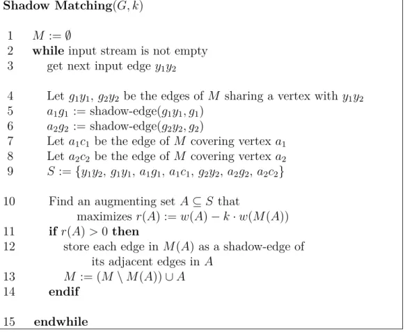
Our algorithm is given in Figure 5.1. Note at first that each edge in the algorithm is denoted by its endpoints, which is done for the sake of simpler considerations in the following on edges having common vertices. Every edge

(37)

5.2. The Algorithm 27

Shadow Matching(G, k) 1 M :=∅

2 while input stream is not empty 3 get next input edge y₁y₂

4 Let g1y1, g2y2 be the edges of M sharing a vertex with y1y2

5 a₁g₁ := shadow-edge(g₁y₁, g₁) 6 a₂g₂ := shadow-edge(g₂y₂, g₂)

7 Let a1c1 be the edge of M covering vertex a1

8 Let a₂c₂ be the edge of M covering vertex a₂ 9 S :={y₁y₂, g₁y₁, a₁g₁, a₁c₁, g₂y₂, a₂g₂, a₂c₂} 10 Find an augmenting set A⊆S that

maximizes r(A) :=w(A)−k·w(M(A)) 11 if r(A)>0 then

12 store each edge in M(A) as a shadow-edge of its adjacent edges in A

13 M := (M \M(A))∪A 14 endif

15 endwhile

Figure 5.1: The algorithm Shadow Matching

c1

c1 c2 c2

a1

a1 a2 a2

g1

g1 g2 g2

y1

y1 y2 y2

S

Figure 5.2: Example of an algorithm’s step. Edges in M are shown in bold, shadow-edges appear in grey.y₁y₂ is the actual input edge shown dashed. The algorithm inserts the augmenting setA ={y1y2, a1g1}intoM. Therefore, the edges M(A) ={a₁c₁, g₁y₁, g₂y₂} are removed from M, they become shadow- edges.

(38)

is well-defined by its endpoints since we assume the input graphGto contain no multi-edges.

The general idea of the algorithm is to keep a valid matching M of G at all times and to decide for each incoming edge y₁y₂ in the input stream if it is inserted into M. This is the case if the weight of y₁y₂ is big compared to the edges already in M sharing a vertex with y₁y₂ and that therefore must be removed from M to incorporatey₁y₂.

This idea so far has already been utilized by one-pass semi-streaming algorithms of Feigenbaum et al. [FKM⁺05b] and McGregor [McG05] seeking a matching in weighted graphs. The algorithm of [FKM⁺05b] is quite simple:

Starting with an empty matchingM, for every input edgee, it examines the at most two edges a, b already in M sharing a vertex with e. If w(e) > k· (w(a)+w(b)) fork = 2,ereplacesaandbinM. The resulting approximation ratio of 6 was improved in [McG05] to 5.828 by changingk to 1.707.

Even if the general approach of our algorithm is similar to both of the above algorithms, there are various important differences.

First, if the algorithms of Feigenbaum et al. [FKM⁺05b] and McGre- gor [McG05] remove an edge from the actual matchingM, this is irrevocable.

Our new algorithm, by contrast, stores some edges that have been in M in the past but were removed from it. To potentially reinsert them intoM, the algorithm memorizes such edges under the name of shadow-edges. For an edge xy inM shadow-edge(xy, a),a ∈ {x, y}, denotes an edge that is stored by the algorithm and shares the vertexawithxy. Every edgexyinM has at most two shadow-edges assigned to it, at most one shadow-edge is assigned to the endpoint xand at most one is assigned to y.

A second main difference is the way of deciding if an edge e is inserted into M or not. In the algorithms of [FKM⁺05b] and [McG05], this decision is based only on the edges in M adjacent to e. Our algorithm takes edges inM as well as shadow-edges in the vicinity of e into account to decide the insertion of e.

Finally, the algorithms of [FKM⁺05b] and [McG05] are limited to the inclusion of the actual input edge into M. By reintegrating shadow-edges, our algorithm can insert up to three edges intoM within a single step.

Let us take a closer look at the algorithm. As an example of a step of the algorithm, Figure 5.2 is given. But note that this picture shows only one possible configuration of the set S. Since non-matching edges in S may be adjacent, S may look different.

(39)

5.2. The Algorithm 29 After reading the actual input edgey₁y₂, the algorithm tags all memorized edges in the vicinity of y₁y₂. This is done in lines 4-8. If an edge is not present, the corresponding tag denotes the null-edge, that is, the empty set of weight zero. Thus, if for example the endpointy₂ of the input edgey₁y₂ is not covered by an edge in M, the identifier g₂y₂ denotes a null-edge as well as its shadow-edgea₂g₂ and the edge a₂c₂. All edges tagged so far are taken into consideration in the remaining part of the loop, they are subsumed to the set S in line 9.

In line 10 all augmenting sets of S are examined. Among these sets the algorithm selects A that maximizes r(A). If r(A) > 0, the edges of A are taken into M and the edges in M sharing a vertex with edges in A are removed from M. We say A is inserted into M, this is done in line 13.

If an augmenting setA is inserted intoM, this is always accompanied by storing the removed edges M(A) as shadow-edges of edges in A in line 12.

More precisely, every edge e in M(A) is assigned as a shadow-edge to every edge in A that shares a vertex with e. If, as in the example given in Fig- ure 5.2,A={y₁y₂, a₁g₁}, the edgeg₁y₁ that is adjacent to both edges in Ais memorized under the name shadow-edge(y₁y₂, y₁) as well as under the name shadow-edge(a₁g₁, g₁). The edgea₁c₁ is stored as shadow-edge(a₁g₁, a₁),g₂y₂ as shadow-edge(y₁y₂, y₂). After inserting A, a₂g₂ is not memorized as a shadow-edge assigned to g₂y₂ any longer since g₂y₂ is not an edge in M after the step. That is indicated in Figure 5.2 by the disappearance of a₂g₂. However, if a₂g₂ was memorized as a shadow-edge of a₂c₂ before, this will also be the case after inserting A.

It is important to note that there is never an edge inM which is a shadow- edge at the same time: Edges only become shadow-edges if they are removed fromM. An edge which is inserted intoM is no shadow-edge anymore, since there is no edge inM it could be assigned to as a shadow-edge.

It is easy to see that our algorithm computes a valid matching of the input graph G.

Corollary 4 Throughout the algorithm Shadow Matching(G, k),M forms a matching of G.

Proof. This is true at the start of the algorithm sinceM =∅. Whenever the algorithm modifies M in line 13, it inserts edges such that no pair of them is adjacent and removes all edges that are adjacent to the newly inserted ones.

Thus,M never includes two adjacent edges. ut

Algorithms for streaming graphs