1. Introduction
The Arctic Ocean is a large freshwater reservoir of the Earth system, gaining freshwater from precipitation, land and the Pacific Ocean and losing it through export of both sea ice and liquid freshwater to the North Atlantic (Serreze et al., 2006). Although similar amounts of Arctic liquid freshwater are exported on both sides of Greenland, Arctic sea ice is mainly exported through Fram Strait, which accounts for nearly one third of the total Arctic freshwater outflow (Haine et al., 2015; Lique et al., 2009; Serreze et al., 2006). One of the pathways in which the Arctic Ocean influences the large-scale global ocean circulation and climate is by modulating the amount of freshwater exported to the North Atlantic where it affects upper ocean stratification and deep water formation (e.g., Aagaard et al., 1985; Arzel et al., 2008). In particular, the first well-documented Great Salinity Anomaly (GSA) in the northern North Atlantic was attributed to excessive sea ice export through Fram Strait (Aagaard & Carmack, 1989; Dickson et al., 1988; Häkkinen, 1993).
Abstract
Understanding the changes of Fram Strait sea ice volume export and responsible processes is crucial due to their climate relevance. In this paper, we disentangled the processes driving the interannual variability and trends of the Fram Strait sea ice volume export in the early 21st century (2001–2019) by using dedicated numerical simulations with the support of observations. The significant decreasing trend in the sea ice volume export is caused by the persistent thinning trend of Arctic sea ice, while the interannual variability of the volume export is predominantly determined by winds. The interannual variability of the volume export can be mainly attributed to the variation in sea ice drift at Fram Strait, while the variation in Fram Strait sea ice thickness also plays an important role. As a result, the atmospheric mode that can better represent the wind variability driving the variability of both the sea ice drift and thickness at Fram Strait can better explain the variability of the sea ice volume export.The wintertime Arctic Oscillation (AO) and Fram Strait sea ice volume export continue to have a strong linkage in the early 21st century. The persistent thinning of Arctic sea ice preconditions events of anomalously low Fram Strait sea ice volume export. One of the extreme events in recent years occurred in 2017/2018. Variation in winds alone would not have caused such an extreme event without the persistent Arctic sea ice thinning.
Plain Language Summary
A strong freshening in the upper ocean of the northern North Atlantic was observed in the 1970s. This event was caused by very high export of sea ice volume through Fram Strait at the end of the 1960s and was the first well-documented Great Salinity Anomaly (GSA).GSAs can have strong impacts on the ocean circulation in the North Atlantic and may also affect weather.
With persistent sea ice thinning in the Arctic Ocean, the export of Arctic sea ice through Fram Strait into the North Atlantic has fallen significantly in the early 21st century. An extreme event of very low sea ice volume export through Fram Strait in recent years is found in this study. This event is due to a combination of winds that tend to reduce sea ice export and the ongoing thinning of Arctic sea ice over past decades. As we expect that Arctic sea ice will continue to decline in a warming world, even stronger events can be anticipated later. Will such events of low sea ice export cause a “positive” GSA, with higher surface salinities in the northern North Atlantic and significant impacts on ocean circulation? This remains to be better monitored and understood.
© 2021. The Authors.
This is an open access article under the terms of the Creative Commons Attribution-NonCommercial License, which permits use, distribution and reproduction in any medium, provided the original work is properly cited and is not used for commercial purposes.
Strait in the Early 21st Century
Qiang Wang1,2 , Robert Ricker1 , and Longjiang Mu2
1Alfred-Wegener-Institut Helmholtz-Zentrum für Polar- und Meeresforschung (AWI), Bremerhaven, Germany,
2Laboratory for Regional Oceanography and Numerical Modeling and Laboratory for Ocean and Climate Dynamics, Pilot National Laboratory for Marine Science and Technology (Qingdao), Qingdao, China
Key Points:
• Arctic sea ice thinning causes a significant decreasing trend in sea ice thickness and volume export at Fram Strait
• Arctic sea ice thinning preconditions events of anomalously low Fram Strait sea ice volume export
• Sea ice volume export over 2001–2019 has close linkages with the Arctic Oscillation in winter and with the Dipole Anomaly for annual means
Supporting Information:
• Figure S1
Correspondence to:
Q. Wang,
Qiang.Wang@awi.de
Citation:
Wang, Q., Ricker, R., & Mu, L. (2021).
Arctic sea ice decline preconditions events of anomalously low sea ice volume export through Fram Strait in the early 21st century. Journal of Geophysical Research: Oceans, 126, e2020JC016607. https://doi.
org/10.1029/2020JC016607 Received 13 JUL 2020 Accepted 6 JAN 2021
Enhanced sea ice export through Fram Strait can facilitate the development of summer low sea ice extent in the Arctic (J. Wang et al., 2009; Williams et al., 2016) and reduce Arctic sea ice thickness, especially north of Greenland (Zamani et al., 2019). Furthermore, changes in Fram Strait sea ice volume export can influence the supply of ocean heat to the Arctic Atlantic Water layer by changing the ocean circulation in the Nordic Seas (Q. Wang et al., 2020). Because of the climate relevance of sea ice export, different techniques have been employed to monitor its changes, including in situ and satellite measurements (Krumpen et al., 2016;
Kwok et al., 2004; Ricker et al., 2018; Spreen et al., 2009; 2020a; Vinje et al., 1998).
The aforementioned observations revealed that sea ice volume export through Fram Strait has strong inter- annual variability, which can be mainly attributed to sea ice drift variability at the Fram Strait gateway (Min et al., 2019; Ricker et al., 2018). Different atmospheric modes have been used to explain the interannual var- iability of sea ice volume export through Fram Strait. Jung and Hilmer (2001) found that the North Atlantic Oscillation (NAO), which in the Arctic region is largely equivalent to the variability represented by the Arctic Oscillation (AO), cannot explain the interannual variability of sea ice volume export during most of the 20th century except its last two decades. They suggested that the eastward movement of the northern activity center of NAO in the later 20th century enhanced the linkage between the variability of NAO and the sea ice vol- ume export. Wind variability associated with the Arctic Dipole Anomaly (DA) can influence Fram Strait sea ice export through its impact on the Transpolar Drift Stream (TDS) (Lei et al., 2016; J. Wang et al., 2009; Wu et al., 2006). In a positive DA phase with a positive sea level pressure (SLP) anomaly on the Greenland side and a negative SLP anomaly over the Eurasian Arctic, more sea ice can be advected toward the Fram Strait and exported there. Considering a time scale of a few decades, Wei et al. (2019) suggest that a regime shift of the at- mospheric circulation from conventional AO/NAO to a dipole-structure pattern in mid-1990s has caused a re- gime shift of Fram Strait sea ice export by changing sea ice motion and main source regions of sea ice outflow.
Although significant trends in sea ice volume transport through Fram Strait were not observed in the past (Spreen et al., 2009), a declining trend has been identified when the analysis was extended to the recent pe- riod by including new sea ice thickness and drift observations (Spreen et al., 2020a). These authors reported that sea ice volume export through Fram Strait has been decreasing with a rate of −648 ± 48 km3yr−1 per decade in the period 1992–2014, which is mainly due to the thinning of the exported sea ice in Fram Strait.
The decrease of sea ice thickness in Fram Strait during the past decades has been confirmed by different observations. The annual mean sea ice thickness in Fram Strait declined by 27% from the 1990s to the period of 2008–2011 (Hansen et al., 2013). Sea ice at the end of the melt season in Fram Strait showed a thinning by more than 50% from 2003 to 2012 (Renner et al., 2014).
The Arctic Ocean is in a new regime in the 21st century as manifested by its much thinner sea ice with much lower coverage than before as a consequence of a persistent long-term declining trend (Comiso et al., 2017;
Kwok, 2018; Laxon et al., 2013; Stroeve et al., 2012). Here, we will investigate the trend and variability of Fram Strait sea ice volume export in the early 21st century (2001–2019) and elucidate their linkages with the Arctic sea ice changes and atmospheric circulation in this period. We use dedicated numerical simulations supported by analyses of recent observations.
The model configurations, observations, and reanalysis data sets used in this paper are described in Sec- tion 2. The results are presented in Section 3, followed by the conclusion in Section 4.
2. Methods and Data
2.1. Numerical Model
In this paper, we employ the Finite Element Sea-ice Ocean Model (FESOM 1.4, Q. Wang et al., 2014, 2018b), a global ocean general circulation model using unstructured triangular meshes (Danilov et al., 2004; Q.
Wang et al., 2008). FESOM solves the primitive equations based on hydrostatic and Boussinesq approxi- mations intended for large-scale climate studies. We use a variable-resolution mesh, which has horizontal resolution of 1° in most parts of the global ocean. The resolution is refined to 24 km north of 45°N and further refined to 4.5 km in the Arctic Ocean. In the vertical, the ocean mesh has 10 m spacing in the upper 100 m, with a total of 47 z-levels. To parameterize diapycnal mixing, the K-profile parameterization scheme (Large et al., 1994) is used. Eddy isopycnal and skew diffusivity is scaled with local horizontal resolution as suggested by Q. Wang et al. (2014). The Smagorinsky (1963) viscosity in the biharmonic form is used.
The sea ice model uses the same surface discretization as the ocean (Danilov et al., 2015), which allows for direct flux exchanges between the ocean and sea ice on the model grid. An updated version of the elas- tic-viscous-plastic (Hunke & Dukowicz, 1997) sea ice rheology is used, with which Arctic sea ice states including small scale linear kinematic features can be reasonably represented at the scale of the model resolu- tion applied (Q. Wang et al., 2016a). The sea ice thermodynamics follow Parkinson and Washington (1979). FESOM has acceptable performance in simulating Arctic sea ice extent and thickness in comparisons with other state-of-the-art global ocean models (Q. Wang et al., 2016b).
The control simulation is a hindcast experiment driven by the JRA55- do (Tsujino et al., 2018) atmosphere reanalysis fields from 1958 to 2019.
This forcing has 0.55° spatial resolution and 3-h temporal resolution. The simulation starts from PHC 3 climatology (Steele et al., 2001) and clima- tological sea ice derived from a previous simulation. This setup is similar to that used in previous studies (Q. Wang et al., 2018a, 2019, 2020) which showed that the Arctic Ocean hydrography and sea ice can be reasonably simulated compared to observations.
In order to unravel the causes of variation in sea ice volume export through Fram Strait, we carried out two sensitivity simulations. In the first one (called wind_vari below), the thermal forcing fields (near sur- face air temperature and downward shortwave and longwave radia- tion) over the Arctic Ocean are replaced by their 3-hourly climatology fields, while winds remain the same as in the control run. The Arctic domain for replacing the forcing is defined by the Arctic gateways near Fram Strait (78°N), Barents Sea Opening (17°E), Davis Strait (66°N), and Bering Strait (66°N). The thermal forcing climatology is obtained by av- eraging the JRA55-do data from 1970 to 1999 for each 3-h segment. By repeatedly using this one-year-long thermal forcing, the sea ice declining trend can be eliminated (Figures 1a and 1b). In the other sensitivity run (called thermal_vari hereafter), the thermal forcing is taken directly from the JRA55-do reanalysis, the same as in the control run, while the wind forcing over the Arctic Ocean is kept the same every year. We follow the recommendation of Stewart et al. (2020) to use the one-year-long winds compiled from 1st May 1990 to 30th April 1991 of JRA55-do, which rep- resent a neutral state of atmospheric circulation. Both sensitivity runs were carried out from 2001 to 2019 starting from the end state of the control run in 2000. We will intercompare the three simulations for the 2001–2019 period.
2.2. Observation and Reanalysis Data
Observational estimates of Fram Strait sea ice volume transport are prone to different uncertainties in measurements of sea ice drift, thickness, and concentration (Spreen et al., 2020a). In this paper, we assess the model re- sults with two independent observational estimates, described by Ricker et al. (2018) and by Spreen et al. (2020a). Ricker et al. (2018) estimated sea ice volume export using satellite-derived products of sea ice thickness (AWI CryoSat-2 sea ice thickness v1.2 [Ricker et al., 2014]), concentration (OSI SAF [EUMETSAT, 2020b]) and velocity (OSI SAF [EUMETSAT, 2020a]) from 2010 to 2017. Monthly ice volume export through Fram Strait was calculated through the gate- way at 82°N (the black transect shown in Figure 1c). In this study, we use an updated version of this data set that now spans 2010–2019, using the most recent AWI CryoSat-2 product version 2.2 (Hendricks & Rick- er, 2019). Changes of the volume export in the overlapping period due to the version update are negligible.
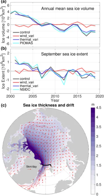
Figure 1. (a) Arctic annual mean sea ice volume in the three simulations and the PIOMAS result (Schweiger et al., 2011). (b) Arctic September sea ice extent in the three simulations and the satellite observation (Fetterer et al., 2017). Anomalies referenced to the respective mean values are shown. (c) Mean sea ice thickness and drift averaged over 2001–2019 in the control run. The black lines (along 82°N and then 20°E) indicate the Fram Strait transect along which sea ice observations (Ricker et al., 2018) are provided. We analyze the model data along this transect, except in Figure 2d which shows results along the 79°N Fram Strait transect.
By combining sea ice thickness from upward looking sonars (ULS) with satellite observations of sea ice drift and concentration, Spreen et al. (2020a) provided Fram Strait sea ice volume export for 1992–2014.
Although annual mean data in 9 years are missing within this period due to unavailability of some of the observations, this is the longest available time series that can be used to compare with model results for assessing long-term trends.
For evaluating sea ice thickness and drift at Fram Strait, the combined model and satellite sea ice thickness (CMST) data set (Mu et al., 2018a, 2019) is also used. CMST is generated by a data assimilation system of the Arctic Ocean based on the Massachusetts Institute of Technology general circulation model (MITgcm) (Losch et al., 2010; Marshall et al., 1997). This system assimilates sea ice concentration data retrieved from Spe- cial Sensor Microwave Imager/Sounder (SSMIS) together with sea ice thickness data from CryoSat-2 and Soil Moisture and Ocean Salinity. Comparisons against sea ice thickness observations from ULS, Ice Mass Balance Buoys, and Operation IceBridge suggest that CMST reproduces reliable temporal and spatial thickness varia- tions (Mu et al., 2018b). The comparison with sea ice drift data retrieved from Sentinel-1 Synthetic Aperture Radar shows that CMST has a smaller bias in Fram Strait than the recently released Polar Pathfinder Daily 25 km EASE-Grid sea ice drift data from NSIDC (Min et al., 2019). CMST provides sea ice drift and thickness records for all months including those without some of the observations for the period 2011–2016, so we can use it to assess the simulated Fram Strait sea ice drift and thickness through the seasons.
The simulated trends of Arctic sea ice volume and extent are compared with the Pan-Arctic Ice Ocean Modeling and Assimilation System (PIOMAS) result (Schweiger et al., 2011) and satellite-based NSIDC sea ice index (Fetterer et al., 2017), respectively. PIOMAS is a regional ocean sea ice model assimilating NSIDC sea ice concentration and sea surface temperature from reanalysis product (Zhang & Rothrock, 2003). Fram Strait sea ice volume export was also derived from PIOMAS output in a study by Selyuzhenok et al. (2020).
For comparison, we will also show this data set.
2.3. Climate Indices
We will investigate the relationship between Fram Strait sea ice volume export and the AO and DA. The standardized monthly AO index is taken from the Climate Prediction Center (NOAA, https://www.cpc.
ncep.noaa.gov/products/precip/CWlink/daily_ao_index/ao.shtml; the AO pattern is available at https://
www.cpc.ncep.noaa.gov/products/precip/CWlink/daily_ao_index/loading.html). The phases of the AO characterize lower/higher than normal SLP over the Arctic Ocean (Thompson & Wallace, 1998). The DA corresponds to the second leading mode of the Empirical Orthogonal Function of the SLP north of 70°N (Kwok et al., 2013; J. Wang et al., 2009; Wu et al., 2006). We calculated the DA index using monthly mean SLP of JRA55-do (Tsujino et al., 2018) over the period 1980–2019. The monthly mean SLP was deseasoned (by removing the mean seasonal cycle) before the calculation. In a positive DA phase, negative SLP anom- alies appear over the Laptev and Kara seas and positive SLP anomalies are close to the Canadian Arctic Archipelago (CAA) and Greenland (Figure S1, supporting information).
3. Results
3.1. Control Run Results
The FESOM control run well represents the declining trend and interannual variability of both Arctic sea ice volume and summer sea ice extent as depicted by the comparison with PIOMAS result and satellite observations in Figures 1a and 1b. The spatial patterns of sea ice thickness (with thicker sea ice north of Greenland and CAA and thinner sea ice toward the Eurasian coast) and sea ice drift (with anticyclonic circulation in the Canada Basin and the TDS toward Fram Strait) shown in Figure 1c are consistent with observations and reanalysis (Kwok, 2018; Min et al., 2019). The magnitudes of the drift speed are similar to those in CMST (Min et al., 2019). In particular, in Fram Strait, sea ice drift closely follows the satellite observation and the CMST result on the monthly time scale (Figure 2a). Even after deseasonalizing the time series, the model's correlation with the CMST result is high (r = 0.91, p < 0.01). A similar performance is found for effective sea ice thickness (thickness averaged over the whole transect) at Fram Strait (Figure 2b).
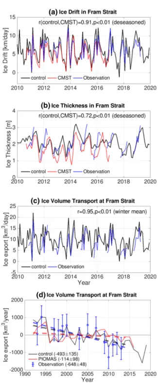
Figure 2. (a) Monthly sea ice drift speed in the Fram Strait gate in the control simulation, CMST reanalysis (Mu et al., 2018a), and the observation (Ricker et al., 2018). (b) The same as (a) but for sea ice thickness. (c) Monthly sea ice volume export at Fram Strait in the control simulation and the observation (Ricker et al., 2018). (d) Annual mean sea ice volume export through Fram Strait in the control simulation, result from PIOMAS reanalysis (Selyuzhenok et al., 2020), and observation (Spreen et al., 2020a). The linear trends (km3/year/decade) for the 1992–2014 period are shown in the figure legend. Note that the model and observational data shown in (a–c) are associated with the Fram Strait transect (black lines) indicated in Figure 1c, while the data in (d) are associated with the 79°N Fram Strait transect. In all figures below the Fram Strait data are associated with the transect indicated in Figure 1c.
The correlation of the deseasonalized sea ice thickness between the con- trol run and the CMST result is also significantly high (r = 0.72, p < 0.01).
Due to good representation of both sea ice thickness and drift, Fram Strait sea ice volume export in the control run compares well with the monthly estimates based on satellite measurements (Figure 2c). The correlation of winter mean sea ice volume export (averaged over six sequential months of NDJFMA when satellite observations are available) between the mod- el and the observation for the period 2010–2019 is as high as r = 0.95 (p < 0.01), indicating that the model adequately reproduces the observed interannual variability.
On a longer time scale, the simulated Fram Strait sea ice volume export in the control run has a significant decreasing trend, consistent with the observation by Spreen et al. (2020a) (Figure 2d). The simulated trend is
−493 ± 135 km3yr−1 per decade in the period 1992–2014. It is weaker than the observational estimate but the difference is within their com- bined uncertainty range. For comparison, the trend in PIOMAS over the same period (Selyuzhenok et al., 2020) is much weaker. Actually, the Fram Strait sea ice volume export in PIOMAS has an increasing trend until about 2005; Afterwards, it decreases similarly as in our control run (Figure 2d).
Overall, the control run is able to reproduce the critical aspects of sea ice inside the Arctic and at Fram Strait as well. It therefore provides a good basis for the sensitivity experiments described in Section 2. We will use these experiments to understand the relationship between changes inside the Arctic and at Fram Strait and reveal the relative contributions to vari- ations in sea ice volume export from winds and thermal forcing.
3.2. Relative Contributions From Winds and Thermal Forcing All the three simulations show interannual variability in their Fram Strait sea ice volume export (Figure 3a). In the following, we focus our study on winter-centered annual means (averaged from July to June of the next year) if not otherwise stated, as sea ice volume export is larg- er in winter. The variability of the wind_vari run explains most of the variability of the control run, as indicated by their high correlation of determination (r2 = 0.85). The control run has a significant decreasing trend of −492 ± 210 km3yr−1 per decade in the Fram Strait sea ice volume export over the period 2001–2019. This trend is nearly the same as that over the period 1992–2014 (Figure 2d). The thermal_vari run has a simi- lar (although slightly stronger) decreasing trend in comparison with the control run, while the wind_vari run has a very weak increasing trend (Figure 3a). Therefore, the decreasing trend of Fram Strait sea ice volume export in the control run is induced by the thermal forcing over the Arctic Ocean.
Similar to the Fram Strait sea ice volume export, the interannual variabil- ity of the effective sea ice thickness in Fram Strait in the control run can be mainly explained by the variability associated with winds (r2 = 0.71, Figure 3b). The thermal forcing explains part of the total variability, but less than winds. In terms of trends of sea ice thickness in Fram Strait, the thermal forcing over the Arctic Ocean is responsible for the decline, as revealed by the fact that the decreasing trends are nearly the same in the control and thermal_vari runs. The linear trend of sea ice thickness in Fram Strait is −0.45 ± 0.12 m Figure 3. (a) Sea ice volume transport anomalies at Fram Strait in the
three simulations and the sum of the two sensitivity runs. The linear trends (km3/year/decade) from 2001 to 2019 are shown in the figure legend. The correlations of determination between the control run and the sensitivity runs for detrended time series are shown at the top of the panel.
(b) The same as (a), but for sea ice thickness in Fram Strait. (c) The same as (a), but for sea ice drift speed in Fram Strait. The linear trends for sea ice thickness (m/decade) and drift speed (km/day/decade) are also shown in the figure legends in (b and c), respectively. The anomalies are referenced to the first year of the shown period. Winter-centered annual mean time series are used in this figure and other figures below.
per decade in the control run, which is close to the observed trend of
−0.42 ± 0.06 m per decade over the period 1990–2014 (Spreen et al., 2020a).
The variability of sea ice drift in Fram Strait (the drift normal to the tran- sect, the same below) is almost fully determined by winds (Figure 3c).
Therefore, it is because Arctic thermal forcing influences the Fram Strait sea ice thickness variability (Figure 3b) that winds do not fully explain the variability of sea ice volume export (Figure 3a). Sea ice drift shows a small increasing trend in both the control and thermal_vari runs (Fig- ure 3c). In the wind_vari run, sea ice drift also has a very weak upward trend. In comparison with the strong interannual variability induced by winds, the trends are not significant. Due to the intrinsic dynamical link- age between sea ice thickness and drift, which is nonlinear, we do not expect to fully reproduce the trend and variability obtained in the control run by summing up the results of the two sensitivity runs, as depicted by Figure 3. However, by using these experiments, we are able to better understand the relative importance of different forcing components as we discussed here. We note that the very weak increasing trend in sea ice drift (Figure 3c) does not lead to a significant upward trend in sea ice area transport through Fram Strait in our simulations (not shown), consistent with Spreen et al. (2020a).
3.3. Interannual Variability
Observations indicate that the variability of Fram Strait sea ice volume export is mainly determined by the variability of Fram Strait sea ice drift, and to a lesser extent by sea ice thickness (Ricker et al., 2018). This is consistently shown by the control run (Figure 4a). The correlation of the detrended sea ice volume transport with the detrended sea ice drift is much higher than with the detrended sea ice thickness (Figure 4a). In the wind_vari run, the variability of sea ice volume export can be mainly attributed to the variability of sea ice drift (Figure 4b). In contrast, in the thermal_vari run, the variability of sea ice volume export can be primar- ily attributed to the variability of sea ice thickness (Figure 4c). The sea ice drift variability, which is mainly induced by winds, overwhelms the sea ice thickness variability, which is induced by both winds and thermal forcing, thus determining the variability of sea ice volume export in the control run (Figure 4a).
Winds lead to strong variability in both sea ice thickness and drift at Fram Strait as shown by the wind_vari run (Figures 3b and 3c). Although the variability in sea ice drift determines the variability of sea ice volume ex- port, the wind-induced sea ice thickness variability also influences the variability of sea ice volume export. Without the impact of sea ice thick- ness variability, the variability of sea ice volume export would be fully determined by sea ice drift, which is not the case in the wind_vari run (Figure 4b). Furthermore, sea ice thickness and drift at Fram Strait are not well correlated with each other (Figure 4b), implying that they are controlled by winds in different regions.
The correlation between Fram Strait sea ice thickness and SLP indicates that a low SLP anomaly over the Eurasian sector of the Arctic Ocean can increase sea ice thickness at Fram Strait (Figure 5a). The SLP gra- dient across the TDS, which was traditionally described by the DA mode or a mode of the central-Arctic SLP gradient, drives the variability of TDS and the amount of sea ice transported toward Fram Strait (Lei et al., 2016; J. Wang et al., 2009; Wu et al., 2006). An increased (decreased) convergence of sea ice toward Figure 4. (a) Normalized winter-centered annual mean sea ice volume
transport, thickness, and speed at Fram Strait in the control simulation.
The correlations of determination between volume transport and thickness/speed are shown at the top of the panel. The correlations are calculated for both detrended and original time series. (b) The same as (a), but for the wind_vari simulation. (c) The same as (a), but for the thermal_
vari simulation.
Fram Strait will increase (decrease) the thickness of sea ice exported. As expected, the Fram Strait sea ice thickness is correlated with the DA index at a relatively high level in the wind_vari run (Figure 6a). Chang- es in winds may influence the location of the TDS and cause sea ice from different regions with different thickness to be advected toward the Fram Strait, thus influencing sea ice thickness in Fram Strait as well.
The correlation between Fram Strait sea ice drift speed and SLP reveals that an active center located at southeast Svalbard is responsible for sea ice drift variability (Figure 5c). That is, meridional winds associat- ed with the SLP gradient across Fram Strait are the main driver for sea ice drift variability. The SLP gradient across Fram Strait has been used in previous studies to reconstruct historical sea ice drift in Fram Strait (Smedsrud et al., 2017). The active center controlling Fram Strait sea ice drift is not well colocated with the active center of AO or DA (Figure 5c), so there is no significant correlation between Fram Strait sea ice drift and AO/DA indices (Figure 6c). However, because the location of the active center of AO changes with time, the correlation between Fram Strait sea ice drift and the AO index is nonstationary as suggested in previous studies (Jung & Hilmer, 2001; Smedsrud et al., 2017). If we extend the period for calculating cor- relation coefficients to include the 1990s, the correlation between annual mean Fram Strait sea ice drift and the AO index is higher (r = 0.4), while it drops again if we further extend the period to also include the 1980s (r = 0.28). Therefore, local winds at Fram Strait are a better predictor for Fram Strait sea ice drift (Figure 5c).
As both sea ice thickness and drift can influence sea ice volume export, the correlation between sea ice volume export and SLP shows a controlling pattern extending from the Barents Sea to the East Siberian Sea (Figure 5e). When the SLP has negative anomalies over both the Eurasian Arctic and the Barents Sea, sea ice volume export will be favorably high. The correlation pattern resembles the DA pattern more than the AO pattern (Figure 5e), so the correlation of the annual mean Fram Strait sea ice volume export with the Figure 5. Correlation coefficient between winter-centered annual mean sea level pressure (SLP) and sea ice (a) thickness, (c) drift speed, and (e) volume transport in the wind_vari simulation. The black curves indicate the p = 0.05 contour lines. (b–f) The same as (a–e) respectively, but for the winter (NDJFMA) mean.
DA index is higher (r = 0.61, p = 0.01) than with the AO index (Figure 6e). Considering only this correla- tion value, without inspecting the correlation patterns shown in Figures 5a, 5c, and 5e), could lead to an incomplete understanding on the role of the DA mode. The DA mode can influence the amount of Arctic sea ice transported toward Fram Strait (J. Wang et al., 2009; Wu et al., 2006), thus influencing the sea ice thickness at Fram Strait, and the changes in sea ice thickness can further influence the Fram Strait sea ice volume export. The impact of the DA mode on Fram Strait sea ice thickness is indeed strong (Figures 5a and 6a). However, the variability of Fram Strait sea ice volume export is mainly determined by Fram Strait sea ice drift, not by Fram Strait sea ice thickness (Figure 4b). Therefore, the significant correlation between sea ice volume export and DA can only be explained by the fact that the DA mode influences not only the sea ice thickness at Fram Strait, but also the Fram Strait sea ice drift when its active center has a spatial extent reaching Fram Strait. Indeed, the DA mode has clear impacts on Fram Strait sea ice drift in years when it is in a strongly positive or negative phase, like in 2007/2008 and 2017/2018 (Figure 6c).
If we only consider the winter months (NDJFMA) when sea ice volume export is large, the SLP patterns controlling Fram Strait sea ice thickness, drift, and volume export are similar to the case of annual means Figure 6. (a) Normalized winter-centered annual mean sea ice thickness at Fram Strait in the wind_vari simulation and the Arctic Oscillation (AO) and Dipole Anomaly (DA) indices. Their correlation coefficients are shown at the top of the panel. (b) The same as (a), but for the winter (NDJFMA) mean. (c and d) The same as (a and b), respectively, but for sea ice drift speed at Fram Strait. (e and f) The same as (a and b), respectively, but for sea ice volume export through Fram Strait.
(Figures 5b, 5d, and 5f). For the winter mean, the sea ice thickness is more strongly correlated with the DA index (Figure 6b), while the sea ice drift is more strongly correlated with the AO index (Figure 6d). The win- ter sea ice volume export through Fram Strait is significantly correlated with the AO index (r = 0.7, p < 0.01, Figure 6f). The strong correlation is because the spatially large SLP pattern over the Eurasian Arctic, which partially resembles the AO pattern, can significantly influence sea ice drift in both the TDS and Fram Strait (Figure 5f). This explains the strong correlation between winter sea ice volume export and the AO index identified based on observed sea ice export by Ricker et al. (2018). The finding here is consistent with that in Williams et al. (2016), who demonstrated winter co-variability between sea ice area export from the Arctic peripheral seas into the central Arctic, Fram Strait sea ice area export, and the AO index.
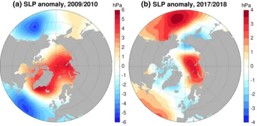
Our analysis leads to the following conclusion: the ability of an atmospheric mode to explain the interannu- al variability of Fram Strait sea ice volume export depends on whether it can well represent the variability of SLP gradients that influence both the sea ice drift and thickness at Fram Strait. This is consistent with the finding that the locations of the active centers of SLP modes are important in determining the variability of Fram Strait sea ice export in previous studies (Jung & Hilmer, 2001; Wei et al., 2019). On average, the location of the AO active center in winter tends to have strong impacts on sea ice export in the early 21st century following the condition in late 20th century; however, it is not the case in every individual year. For example, AO was in an anomalously low phase in 2009/2010 (Figure 6) but neither the SLP gradient across the TDS nor across the Fram Strait is strong due to the location of the AO active center (Figure 7a). As a result, the Fram Strait sea ice volume export was not anomalously low in that year despite the very low AO phase. The analysis in this section is based on the wind_vari run but the correlation maps using the control run are similar to those in Figure 5 if we detrend the time series (not shown), as the interannual variabilities of sea ice drift, thickness and volume ex- port are largely determined by winds (Figure 3).
3.4. Decreasing Sea Ice Volume Export
As shown by Figure 3, there is a significant decreasing trend in the Fram Strait sea ice volume export due to Fram Strait sea ice thinning caused by Arctic thermal forcing in the period 2001–2019. In the thermal_vari run, the sea ice thickness at Fram Strait closely follows the variability and the trend of Arctic mean sea ice thickness (Figure 8). Furthermore, the trend of sea ice thickness in Fram Strait is nearly the same in the control and thermal_vari runs (Figure 3b). Therefore, for the long-term trend of the Fram Strait sea ice volume export, the Arctic thermal forcing and the Arctic mean sea ice thickness are very good predictors. For interannual Figure 7. Sea level pressure (SLP) anomaly for winter-centered annual mean of (a) 2009/2010 and (b) 2017/2018.
Figure 8. Normalized sea ice thickness averaged over the Arctic Ocean and in the Fram Strait in the thermal_vari simulation.
variability of the Fram Strait sea ice volume export, as wind-induced variability tends to overwhelm the variability induced by thermal forcing on an interannual time scale, winds are a potential predictor.
The control run reveals that the Fram Strait sea ice volume export was anomalously low in 2017/2018 rel- ative to the first two decades of the 21st century (Figure 3a). There was a strong positive SLP anomaly over the Eurasian Arctic in that period (Figure 7b), which reduced sea ice thickness at Fram Strait (Figures 6a and 6b), and slowed down sea ice drift at Fram Strait (Figures 6c and 6d). In the wind_vari run, the sea ice volume export in 2017/2018 was the lowest in the studied period owing to the strong positive SLP anomaly, but it was only slightly lower than in other low export years (Figures 6e and 6f). It was due to the persis- tent Arctic sea ice thinning over past decades that this year turned out to have an anomalously low sea ice volume export as shown by the control run (Figure 3a). Given the expected climate warming in the coming decades, a continuing decrease in the Fram Strait sea ice volume export is expected, and we also foresee that more record lows in sea ice volume export will be observed.
As sea ice volume export has been decreasing, the export did not contribute to the declining trend of Arctic sea ice volume. However, our sensitivity experiments agree with previous studies on the role of winds in individual events of low Arctic sea ice extent in summer (e.g., Lindsay et al., 2009; J. Wang et al., 2009). This is most obvious in 2007 in our simulations, when winds had a significant contribution to the low sea ice extent in September (Figure 1b).
4. Conclusions
In this paper, we investigated the variability and trend of Fram Strait sea ice volume export in the early 21st century by using numerical simulations with the support of observations. We focused on the attri- bution of the variability, trend, and extreme events. Our control hindcast simulation well reproduced the observed decreasing trend and variability of the Fram Strait sea ice volume export. The simulated trend is
−493 ± 135 km3yr−1 per decade over the 1992–2014 period, and the observation is −648 ± 48 km3yr−1 per decade (Spreen et al., 2020a). Considering that the long-term mean Fram Strait sea ice volume export is 2,400 ± 640 km3yr−1 (Spreen et al., 2020a), the decreasing trend represents a large change.
We found that the overall thinning trend of sea ice in the Arctic Ocean, which is mainly driven by atmos- pheric warming, is responsible for the significant decreasing trend in the Fram Strait sea ice thickness and volume export in the past two decades. Although thinner and less compact sea ice causes a small increasing trend in sea ice drift, the sea ice volume export decreases. Fram Strait sea ice volume export is a budget term of Arctic sea ice volume, but the trend of this budget term follows the trend of the Arctic sea ice thickness (and volume) that is determined by the warming of the atmosphere.
Winds determine the interannual variability of Fram Strait sea ice volume export by influencing sea ice drift both inside the Arctic Ocean and at Fram Strait. By influencing the TDS, the SLP gradient across the TDS influences the amount of sea ice transported toward the Fram Strait, thus the sea ice thickness at Fram Strait. The SLP gradient across Fram Strait primarily determines the variability of sea ice drift at Fram Strait.
The interannual variability of Fram Strait sea ice volume export generally follows the variability of sea ice drift at Fram Strait as also suggested by previous observations (Ricker et al., 2018); however, the sea ice thickness variability at Fram Strait also influences the export variability. Therefore, the atmospheric mode that better explains the variability of both the Fram Strait sea ice thickness and drift is the better predictor of varying Fram Strait sea ice volume export. We found that the AO well explains the interannual variability of the Fram Strait sea ice volume export for the winter time in the early 21st century, while the DA better explains the variability of annual mean export. Jung and Hilmer (2001) suggested that the NAO/AO could explain the wintertime variability of the Fram Strait sea ice volume export in the last two decades of the 20th century due to the northeastward shift of the AO variability center; our study indicates that this situation has continued into the early 21st century. Note that the active center of the AO can shift to locations where it has only minor impacts on the Fram Strait sea ice volume export in some years.
An anomalously low sea ice volume export was found in 2017/2018 in terms of both winter export and winter-centered annual mean export (for the summer-centered annual mean export, the minimum was in
2018). This event concurred with a strong positive SLP anomaly over the Eurasian Arctic which extended to the western Barents Sea. However, the anomalous winds associated with this SLP anomaly would not have caused the export low to such an extreme extent without the persistent thinning trend of Arctic sea ice. That is, the Arctic sea ice thinning not only preconditions record low Arctic sea ice cover (Lindsay et al., 2009;
Parkinson & Comiso, 2013), but also preconditions anomalously low sea ice volume export through Fram Strait as revealed in our study. We can expect a continuing decrease in sea ice volume export and stronger events of low export in a warming world. Their impacts on the ocean circulation and possible occurrence of
“positive” GSAs in the subpolar North Atlantic need to be better monitored and understood. We anticipate that negative GSAs induced by anomalously high sea ice volume export found in the past have a relatively low probability of happening again, because the amount of sea ice volume exported in recent high export events is already less than previous normal states.
Data Availability Statement
The model data used in figures can be found at http://doi.org/10.5281/zenodo.3942078. Observational and reanalysis data used for model assessment were obtained from respective sites described in the following references: Fetterer et al. (2017); Schweiger et al. (2011); EUMETSAT (2020b), EUMETSAT (2020a), Spreen et al. (2020b), Ricker et al. (2018), Hendricks and Ricker (2019), Mu et al. (2018a), Mu et al. (2019), Selyu- zhenok et al. (2020).
References
Aagaard, K., & Carmack, E. C. (1989). The role of sea ice and other fresh-water in the Arctic circulation. Journal of Geophysical Research, 94, 14485–14498.
Aagaard, K., Swift, J. H., & Carmack, E. (1985). Thermohaline circulation in the Arctic Mediterranean seas. Journal of Geophysical Re- search, 90, 4833–4846.
Arzel, O., Fichefet, T., Goosse, H., & Dufresne, J.-L. (2008). Causes and impacts of changes in the Arctic freshwater budget during the 20th and 21st centuries in an AOGCM. Climate Dynamics, 30, 37–58.
Comiso, J. C., Meier, W. N., & Gersten, R. (2017). Variability and trends in the Arctic sea ice cover: Results from different techniques. Jour- nal of Geophysical Research: Oceans, 122, 6883–6900. https://doi.org/10.1002/2017JC012768
Danilov, S., Kivman, G., & Schröter, J. (2004). A finite-element ocean model: Principles and evaluation. Ocean Modelling, 6, 125–150.
Danilov, S., Wang, Q., Timmermann, R., Iakovlev, N., Sidorenko, D., Kimmritz, M., et al. (2015). Finite-Element Sea Ice Model (FESIM), version 2. Geoscientific Model Development, 8, 1747–1761.
Dickson, R., Meincke, J., Malmberg, S., & Lee, A. J. (1988). The great salinity anomaly in the Northern North-Atlantic 1968-1982. Progress in Oceanography, 20, 103–151.
EUMETSAT. (2020). Ocean and sea ice satellite application facility, sea ice concentration product. Retrieved from ftp://osisaf.met.no/
archive/ice/conc
EUMETSAT. (2020). Ocean and sea ice satellite application facility, low resolution sea ice drift product. Retrieved from ftp://osisaf.met. no/
archive/ice/drift_lr
Fetterer, F., Knowles, K., Meier, W., Savoie, M., & Windnage, A. K. (2017). Sea ice index, Version 3. Boulder, CO: NSIDC: National Snow and Ice Data Center.
Haine, T., Curry, B., Gerdes, R., Hansen, E., Karcher, M., Lee, C., et al. (2015). Arctic freshwater export: Status, mechanisms, and prospects.
Global and Planetary Change, 125, 13–35.
Häkkinen, S. (1993). An Arctic source for the great salinity anomaly: A simulation of the Arctic ice-ocean system for 1955–1975. Journal of Geophysical Research, 98, 16397–16410.
Hansen, E., Gerland, S., Granskog, M. A., Pavlova, O., Renner, A. H. H., Haapala, J., et al. (2013). Thinning of Arctic sea ice observed in Fram Strait: 1990–2011. Journal of Geophysical Research: Oceans, 118, 5202–5221. https://doi.org/10.1002/jgrc.20393
Hendricks, S., & Ricker, R. (2019). Product user guide and algorithm specification: AWI CryoSat-2 sea ice thickness (version 2.2) (Technical Report). Alfred Wegener Institute.
Hunke, E., & Dukowicz, J. (1997). An elastic-viscous-plastic model for sea ice dynamics. Journal of Physical Oceanography, 27, 1849–1867.
Jung, T., & Hilmer, M. (2001). The link between the North Atlantic oscillation and Arctic Sea ice export through Fram Strait. Journal of Climate, 14, 3932–3943.
Krumpen, T., Gerdes, R., Haas, C., Hendricks, S., Herber, A., Selyuzhenok, V., et al. (2016). Recent summer sea ice thickness surveys in Fram Strait and associated ice volume fluxes. The Cryosphere, 10, 523–534.
Kwok, R. (2018). Arctic sea ice thickness, volume, and multiyear ice coverage: Losses and coupled variability (1958–2018). Environmental Research Letters, 13, 105005. https://doi.org/10.1088/1748-9326/aae3ec
Kwok, R., Cunningham, G. F., & Pang, S. S. (2004). Fram Strait sea ice outflow. Journal of Geophysical Research, 109, C01009. https://doi.
org/10.1029/2003JC001785
Kwok, R., Spreen, G., & Pang, S. (2013). Arctic sea ice circulation and drift speed: Decadal trends and ocean currents. Journal of Geophys- ical Research: Oceans, 118(5), 2408–2425. https://doi.org/10.1002/jgrc.20191
Large, W. G., Mcwilliams, J. C., & Doney, S. C. (1994). Oceanic vertical mixing – A review and a model with a nonlocal boundary-layer parameterization. Reviews of Geophysics, 32, 363–403.
Acknowledgments
This work is supported by the German Helmholtz Climate Initiative REKLIM (Regional Climate Change). The authors thank Charles Brunette, the anonymous reviewer and the editor for helpful suggestions.
Laxon, S. W., Giles, K. A., Ridout, A. L., Wingham, D. J., Willatt, R., Cullen, R., et al. (2013). CryoSat-2 estimates of Arctic sea ice thickness and volume. Geophysical Research Letters, 40, 732–737. https://doi.org/10.1002/grl.50193
Lei, R., Heil, P., Wang, J., Zhang, Z., Li, Q., & Li, N. (2016). Characterization of sea-ice kinematic in the Arctic outflow region using buoy data. Polar Research, 35, 22658. https://doi.org/10.3402/polar.v35.22658
Lindsay, R. W., Zhang, J., Schweiger, A., Steele, M., & Stern, H. (2009). Arctic sea ice retreat in 2007 follows thinning trend. Journal of Climate, 22, 165–176.
Lique, C., Treguier, A. M., Scheinert, M., & Penduff, T. (2009). A model-based study of ice and freshwater transport variability along both sides of Greenland. Climate Dynamics, 33, 685–705.
Losch, M., Menemenlis, D., Campin, J.-M., Heimbach, P., & Hill, C. (2010). On the formulation of sea-ice models. part 1: Effects of different solver implementations and parameterizations. Ocean Modelling, 33, 129–144.
Marshall, J., Adcroft, A., Hill, C., Perelman, L., & Heisey, C. (1997). A finite-volume, incompressible Navier Stokes model for studies of the ocean on parallel computers. Journal of Geophysical Research, 102, 5753–5766.
Min, C., Mu, L., Yang, Q., Ricker, R., Shi, Q., Han, B., et al. (2019). Sea ice export through the Fram Strait derived from a combined model and satellite data set. The Cryosphere, 13, 3209–3224.
Mu, L., Losch, M., Yang, Q., Ricker, R., Losa, S., & Nerger, L. (2018). The Arctic combined model and satellite sea ice thickness (CMST) data- set. https://doi.org/10.1594/PANGAEA.891475
Mu, L., Losch, M., Yang, Q., Ricker, R., Losa, S. N., & Nerger, L. (2018). Arctic-wide sea ice thickness estimates from combining satellite re- mote sensing data and a dynamic ice-ocean model with data assimilation during the CryoSat-2 period. Journal of Geophysical Research:
Oceans, 123, 7763–7780. https://doi.org/10.1029/2018JC014316
Mu, L., Losch, M., Yang, Q., Ricker, R., Loza, S. N., & Nerger, L. (2019). The Arctic sea ice drift simulation from October 2010 to December 2016. https://doi.org/10.1594/PANGAEA.906973
Parkinson, C. L., & Comiso, J. C. (2013). On the 2012 record low Arctic sea ice cover: Combined impact of preconditioning and an August storm. Geophysical Research Letters, 40, 1356–1361. https://doi.org/10.1002/grl.50349
Parkinson, C. L., & Washington, W. M. (1979). A large-scale numerical model of sea ice. Journal of Geophysical Research, 84, 311–337.
Renner, A. H. H., Gerland, S., Haas, C., Spreen, G., Beckers, J. F., Hansen, E., et al. (2014). Evidence of Arctic sea ice thinning from direct observations. Geophysical Research Letters, 41, 5029–5036. https://doi.org/10.1002/2014GL060369
Ricker, R., Girard-Ardhuin, F., Krumpen, T., & Lique, C. (2018). Satellite-derived sea ice export and its impact on Arctic ice mass balance.
The Cryosphere, 12, 3017–3032.
Ricker, R., Hendricks, S., Helm, V., Skourup, H., & Davidson, M. (2014). Sensitivity of CryoSat-2 Arctic sea-ice freeboard and thickness on radar-waveform interpretation. The Cryosphere, 8, 1607–1622.
Schweiger, A., Lindsay, R., Zhang, J., Steele, M., Stern, H., & Kwok, R. (2011). Uncertainty in modeled Arctic sea ice volume. Journal of Geophysical Research, 116, C00D06. https://doi.org/10.1029/2011JC007084
Selyuzhenok, V., Bashmachnikov, I., Ricker, R., Vesman, A., & Bobylev, L. (2020). Sea ice volume variability and water temperature in the Greenland Sea. The Cryosphere, 14, 477–495.
Serreze, M. C., Barrett, A. P., Slater, A. G., Woodgate, R. A., Aagaard, K., Lammers, R. B., et al. (2006). The large-scale freshwater cycle of the Arctic. Journal of Geophysical Research, 111, C11010. https://doi.org/10.1029/2005JC003424
Smagorinsky, J. (1963). General circulation experiments with the primitive equations: I. The basic experiment. Monthly Weather Review, 91, 99–164.
Smedsrud, L. H., Halvorsen, M. H., Stroeve, J. C., Zhang, R., & Kloster, K. (2017). Fram Strait sea ice export variability and September Arctic sea ice extent over the last 80 years. The Cryosphere, 11, 65–79.
Spreen, G., de Steur, L., Divine, D., Gerland, S., Hansen, E., & Kwok, R. (2020). Arctic sea ice volume export through Fram Strait from 1992 to 2014. Journal of Geophysical Research: Oceans, 125, e2019JC016039. https://doi.org/10.1029/2019JC016039
Spreen, G., de Steur, L., Divine, D., Hansen, E., Gerland, S., & Kwok, R. (2020). Fram Strait sea ice volume transport based on ULS ice thick- ness and satellite ice drift. Norwegian Polar Institute. https://doi.org/10.21334/npolar.2020.696b80db
Spreen, G., Kern, S., Stammer, D., & Hansen, E. (2009). Fram Strait sea ice volume export estimated between 2003 and 2008 from satellite data. Geophysical Research Letters, 36, L19502. https://doi.org/10.1029/2009GL039591
Steele, M., Morley, R., & Ermold, W. (2001). PHC: A global ocean hydrography with a high quality Arctic Ocean. Journal of Climate, 14, 2079–2087.
Stewart, K. D., Kim, W. M., Urakawa, S., Hogg, A. M., Yeager, S., Tsujino, H., et al. (2020). JRA55-do-based repeat year forcing datasets for driving ocean–sea-ice models. Ocean Modelling, 147, 101557. https://doi.org/10.1016/j.ocemod.2019.101557
Stroeve, J. C., Kattsov, V., Barrett, A., Serreze, M., Pavlova, T., Holland, M., & Meier, W. N. (2012). Trends in Arctic sea ice extent from CMIP5, CMIP3 and observations. Geophysical Research Letters, 39, L16502. https://doi.org/10.1029/2012GL052676
Thompson, D. W. J., & Wallace, J. M. (1998). The Arctic Oscillation signature in the wintertime geopotential height and temperature fields.
Geophysical Research Letters, 25, 1297–1300.
Tsujino, H., Urakawa, S., Nakano, H., Small, R. J., Kim, W. M., Yeager, S. G., et al. (2018). JRA-55 based surface dataset for driving ocean–
sea-ice models (JRA55-do). Ocean Modelling, 130, 79–139. https://doi.org/10.1016/j.ocemod.2018.07.002
Vinje, T., Nordlund, N., & Kvambekk, A. (1998). Monitoring ice thickness in Fram Strait. Journal of Geophysical Research, 103, 10437–10449.
Wang, Q., Danilov, S., Jung, T., Kaleschke, L., & Wernecke, A. (2016). Sea ice leads in the Arctic Ocean: Model assessment, interannual variability and trends. Geophysical Research Letters, 43, 7019–7027. https://doi.org/10.1002/2016GL068696
Wang, Q., Ilicak, M., Gerdes, R., Drange, H., Aksenov, Y., Bailey, D. A., et al. (2016). An assessment of the Arctic Ocean in a suite of inter- annual CORE-II simulations. Part I: Sea ice and solid freshwater. Ocean Modelling, 99, 110–132.
Wang, Q., Danilov, S., & Schröter, J. (2008). Finite element ocean circulation model based on triangular prismatic elements, with applica- tion in studying the effect of vertical discretization. Journal of Geophysical Research, 113, C05015. https://doi.org/10.1029/2007JC004482 Wang, Q., Danilov, S., Sidorenko, D., Timmermann, R., Wekerle, C., Wang, X., et al. (2014). The Finite Element Sea Ice-Ocean Model (FES-
OM) v.1.4: Formulation of an ocean general circulation model. Geoscientific Model Development, 7, 663–693.
Wang, Q., Wekerle, C., Danilov, S., Koldunov, N., Sidorenko, D., Sein, D., et al. (2018). Arctic sea ice decline significantly contributed to the unprecedented liquid freshwater accumulation in the Beaufort Gyre of the Arctic Ocean. Geophysical Research Letters, 45, 4956–4964.
https://doi.org/10.1029/2018GL077901
Wang, Q., Wekerle, C., Danilov, S., Wang, X., & Jung, T. (2018). A 4.5 km resolution Arctic Ocean simulation with the global multi-resolu- tion model FESOM 1.4. Geoscientific Model Development, 11, 1229–1255.
Wang, Q., Wekerle, C., Danilov, S., Sidorenko, D., Koldunov, N., Sein, D.., et al. (2019). Recent sea ice decline did not significantly increase the total liquid freshwater content of the Arctic Ocean. Journal of Climate, 32, 15–32.
Wang, Q., Wekerle, C., Wang, X., Danilov, S., Koldunov, N., Sein, D. V, et al. (2020). Intensification of the Atlantic Water supply to the Arctic Ocean through Fram Strait induced by Arctic sea ice decline. Geophysical Research Letters, 47, e2019GL086682. https://doi.
org/10.1029/2019GL086682
Wang, J., Zhang, J., Watanabe, E., Ikeda, M., Mizobata, K., Walsh, J. E., et al. (2009). Is the Dipole Anomaly a major driver to record lows in Arctic summer sea ice extent? Geophysical Research Letters, 36, L05706. https://doi.org/10.1029/2008GL036706
Wei, J., Zhang, X., & Wang, Z. (2019). Reexamination of Fram Strait sea ice export and its role in recently accelerated Arctic sea ice retreat.
Climate Dynamics, 53, 1823–1841.
Williams, J., Tremblay, B., Newton, R., & Allard, R. (2016). Dynamic preconditioning of the minimum September sea-ice extent. Journal of Climate, 29, 5879–5891.
Wu, B., Wang, J., & Walsh, J. (2006). Dipole Anomaly in the winter Arctic atmosphere and its association with sea ice motion. Journal of Climate, 19, 210–225.
Zamani, B., Krumpen, T., Smedsrud, L. H., & Gerdes, R. (2019). Fram Strait sea ice export affected by thinning: Comparing high-resolution simulations and observations. Climate Dynamics, 53, 3257–3270.
Zhang, J., & Rothrock, D. A. (2003). Modeling global sea ice with a thickness and enthalpy distribution model in generalized curvilinear coordinates. Monthly Weather Review, 131, 845–861.