Nemo-Nordic 1.0: a NEMO-based ocean model for the Baltic and North seas – research and operational applications

(1)

https://doi.org/10.5194/gmd-12-363-2019

Nemo-Nordic 1.0: a NEMO-based ocean model for the Baltic and North seas – research and operational applications

Robinson Hordoir^1,2, Lars Axell³, Anders Höglund³, Christian Dieterich³, Filippa Fransner^5,4,2, Matthias Gröger³, Ye Liu³, Per Pemberton³, Semjon Schimanke³, Helen Andersson³, Patrik Ljungemyr³, Petter Nygren³,

Saeed Falahat³, Adam Nord³, Anette Jönsson³, Iréne Lake³, Kristofer Döös⁵, Magnus Hieronymus³, Heiner Dietze⁶, Ulrike Löptien⁶, Ivan Kuznetsov⁷, Antti Westerlund⁸, Laura Tuomi⁸, and Jari Haapala⁸

1Institute of Marine Research, Bergen, Norway

2Bjerknes Centre for Climate Research, Bergen, Norway

3Swedish Meteorological and Hydrological Institute, Norrköping, Sweden

4Geophysical Institute, Bergen University, Bergen, Norway

5Department of Meteorology, Stockholm University and Bolin Centre for Climate Research, Stockholm, Sweden

6GEOMAR, Helmholtz Centre for Ocean Research, Kiel, Germany

7Institute of Coastal Research, Helmholtz-Zentrum, Geesthacht, Germany

8Finnish Meteorological Institute, Helsinki, Finland

Correspondence:Robinson Hordoir (robinson.hordoir@hi.no) Received: 5 January 2018 – Discussion started: 5 April 2018

Revised: 10 December 2018 – Accepted: 21 December 2018 – Published: 21 January 2019

Abstract.We present Nemo-Nordic, a Baltic and North Sea model based on the NEMO ocean engine. Surrounded by highly industrialized countries, the Baltic and North seas and their assets associated with shipping, fishing and tourism are vulnerable to anthropogenic pressure and climate change.

Ocean models providing reliable forecasts and enabling climatic studies are important tools for the shipping infrastruc- ture and to get a better understanding of the effects of climate change on the marine ecosystems. Nemo-Nordic is intended to be a tool for both short-term and long-term simulations and to be used for ocean forecasting as well as process and climatic studies. Here, the scientific and technical choices within Nemo-Nordic are introduced, and the reasons behind the design of the model and its domain and the inclusion of the two seas are explained. The model’s ability to represent barotropic and baroclinic dynamics, as well as the vertical structure of the water column, is presented. Biases are shown and discussed. The short-term capabilities of the model are presented, especially its capabilities to represent sea level on an hourly timescale with a high degree of accuracy. We also show that the model can represent longer timescales, with a focus on the major Baltic inflows and the variability in deep- water salinity in the Baltic Sea.

1 Introduction

The Baltic Sea is a semi-enclosed sea that is heavily influenced by freshwater input from large continental rivers.

The large freshwater input and the narrow connection with the North Sea and the Atlantic Ocean through the Danish Straits gives the Baltic Sea its brackish characteristics with a strongly stratified water column and a water residence time of ca. 40 years (Döös et al., 2004).

Due to the long residence time and the strong stratification, the Baltic Sea ecosystem is vulnerable to anthropogenic pressure. As a result of large nutrient inputs the sea is to- day classified as eutrophied (Andersen et al., 2017), and a spreading of anoxic bottom waters has been observed during the last century (Carstensen et al., 2014). Eutrophication and anoxia can have severe impacts on the ecosystem. The cod, for example, which is a economically important fish species (Köster et al., 2003; Wieland et al., 1994), suffers from the effect of anoxic deep waters as its eggs are found in the Baltic Sea deep waters. Further, although all underly- ing mechanisms are still not clear, increases in cyanobacte- ria blooms are often related to eutrophication (Vahtera et al., 2007).

(2)

The vertical structure of the Baltic Sea and its ecosystem is in the long term influenced by inflows of salt water masses from the North Sea through the Danish Straits (e.g.

Boesch et al., 2006; Eilola et al., 2009; Fonselius and Valder- rama, 2003; Neumann et al., 2012; Pawlak et al., 2009; Was- mund and Uhlig, 2003; Fredrik Wulff, 1990). The timescale of a typical “major Baltic inflow” (hereafter MBI), which provides salt and oxygen to the deepest parts of the Baltic Sea and fuels the Baltic Sea baroclinic circulation (Döös et al., 2004), is on the order of 40 days (Schimanke et al., 2014). MBIs are barotropic in nature, and the variability in the barotropic circulation on timescales of hours to days can affect the Baltic Sea ecosystem on timescales up to several decades or a whole century.

Fuelled by advances in computer hardware, the quest towards a more comprehensive understanding of the crucial ventilation of the Baltic Sea has been aided by simulations of inflows with numerical general ocean circulation models (Hordoir et al., 2015), and it has been shown that these inflows are closely correlated to the sea surface height (hereafter SSH) variability in both the Baltic and the North Sea (Gustafsson and Andersson, 2001). An ocean model that provides a consistent representation of the Baltic Sea long-term ecosystem with its specific haline dynamics and stratification on one side and that allows us to make an accurate forecast of SSH for the Baltic and the North Sea basin is not incom- patible: it is complementary.

Compared to the Baltic Sea, the North Sea is a dynamical region with a water residence time of only a few years (Otto et al., 1990). It is characterized by strong tidal currents and a general cyclonic large-scale circulation pattern (Winther and Johannessen, 2006) with major inflow along the British Isles in the western part of northern boundary and an outflow along the Norwegian Channel in the east.

Strong local inflow of 0.29 Sv (sverdrup) occurs via the Pentland Firth and the straits of Fair Isle, and 1.33 Sv is obtained east of the Shetland Islands (Thomas et al., 2005).

In addition to this, around 0.15 Sv comes through the En- glish Channel (Otto et al., 1990; Thomas et al., 2005) and around 0.016 Sv is received from the Baltic Sea (Stigebrandt, 2001). Outflow to the North Atlantic at the northern end of the Norwegian Channel amounts to 1.79 Sv. Unlike the Baltic Sea, the North Sea is not permanently stratified. Dur- ing winter, enhanced wind-induced mixing in combination with convective mixing maintains well-mixed conditions almost everywhere with the exception of the Norwegian Chan- nel region where fresh outflow waters from the Baltic Sea dominate (Schrum, 2001; Schrum et al., 2003; Ådlandsvik and Bentsen, 2007; Huthnance et al., 2009; Holt et al., 2010;

Mathis et al., 2013; Emeis et al., 2015; Mathis et al., 2015).

During summer, the deeper parts of the central and northern North Sea experience a strong thermal stratification (Mathis et al., 2013), whereas the shallow southern North Sea remains mostly well mixed throughout the year though short- term stratified periods are possible (Baretta-Bekker et al.,

2009). The timing and intensity of the seasonal stratification play an important role in biogeochemical processes as they influence primary production, the start of the spring phytoplankton bloom and nutrient cycling in the North Sea (Pätsch and Kühn, 2008; Holt et al., 2012; Daewel and Schrum, 2013; Gröger et al., 2013).

For both the North Sea (Mathis et al., 2013; Graham et al., 2017) and the Baltic Sea (Meier et al., 2003; Burchard et al., 2009; Hordoir et al., 2015), there are a number of models of different complexity. Because the two seas differ so much in their oceanographical and biogeochemical characteristics, it is plausible to set up separate models specific to each region and to prescribe lateral boundaries at a reasonable location in the transition zone between the two seas. However, recent studies provide evidence that the simulation of the Sk- agerrak and Kattegat hydrography are often problematic in these model set-ups (Pätsch et al., 2017). As the dynamics in this transition zone between the Baltic and the North Sea are essential for a realistic simulation of MBIs, a combined Baltic–North Sea model is necessary to better understand MBI dynamics and their impact on the Baltic and the North Sea physics and ecosystem. Especially for climate scenario simulations, it is more appropriate to explicitly simulate po- tential changes in the Kattegat–Skagerrak region than relying on a present-day climatological prescription. Further, ocean models that include only the North Sea do not take into account the interaction with the Baltic Sea, and therefore rely on a freshwater provision to the North Sea that is not accurate in strength or in time (Hordoir et al., 2013).

Early attempts of combined North Sea–Baltic Sea modelling were limited by a relatively coarse resolution (approx. 11 000 m, or 6 nm) and constrained to short-term simulations of 1 year (Schrum and Backhaus, 2011). Only recently, attempts have been made to include the two seas in one model set-up for longer periods and at a high resolution.

Daewel and Schrum (2013) used a coupled hydrodynamic–

biogeochemical model and concluded that coupled Baltic and North Sea model set-ups can help to improve the performance in the Skagerrak area. Moreover, the model reason- ably simulated the MBIs during the hindcast period (Daewel and Schrum, 2013). Gräwe et al. (2015b) presented a hydrodynamic model using adaptive vertical coordinates and with a resolution of 1852 m (or 1 nm). The authors found the mean state for the period 1997–2012 as well as the timing and amplitude of MBIs were well represented by the model. Tian et al. (2013) as well as Pham et al. (2014) each presented a hydrodynamic model coupled to an atmospheric model but they focused more on atmospheric dynamics and air–sea in- teractions than on oceanographic topics.

In the present article, we provide a description and validation of Nemo-Nordic in its first mature version, Nemo- Nordic 1.0, based on NEMO 3.6. Nemo-Nordic is divided into two resolutions of 2 nautical miles (3704 m) and 1 nautical mile (1852 m). First prototype versions were already used for process studies in Hordoir et al. (2013); Hordoir

(3)

et al. (2015) or to specifically investigate the added value of interactive air–sea exchange of mass and energy fluxes (Gröger et al., 2015). The present version is the first reference used both for research and forecast. This article provides a full validation of both barotropic and baroclinic dynamics, it shows the qualities and biases of the model. It is also a milestone that will be used for further development at a time when Nemo-Nordic extends beyond SMHI (Nor- wegian Institute of Marine Research, Danish Meteorological Institute, Finnish Meteorological Institute, Deutsche Wetter- dienst, German Federal Maritime and Hydrographic Agency BSH). Further developments are to be done in the different European institutions within the Copernicus framework, for example, for operational applications and for research.

Nemo-Nordic is a NEMO (Madec and the NEMO system team, 2015) based ocean model for the Baltic and the North Sea that can be used for climate, oceanographic process study and operational oceanographic applications. Nemo-Nordic has been designed to be an advanced compromise to provide forecasts or study Baltic and/or North Sea dynamics at various timescales (operational or climate timescales), with a representation of processes occurring in both basins, including overflows and sea ice, within a reasonable range of computing resources. The inclusion of both seas makes it possible to study the exchange between the two seas because the boundary conditions of the model are far enough from where this exchange occurs, unlike, for example, a Baltic Sea only ocean model (Meier et al., 2003). Unlike Nemo-Nordic, the model described by Meier et al. (2003) is in any case limited by its linear free surface, which produces conservation errors for the Baltic Sea in long-term simulations, and prevents any possibility of representing ocean dynamics properly in any region of higher sea level variability, such as the Kattegat, the Skagerrak and the entire North Sea.

Nemo-Nordic is also not the first model to include both the Baltic and the North Sea basins; one could cite Funkquist and Kleine (2007) or Madsen et al. (2015) as examples of models that already do. However, these models do not permit us to represent the main driver of the Baltic Sea ecosystem: the dense overflows that feed its very specific sill-bounded estuarine circulation; this circulation is difficult to represent inz coordinates since such coordinate systems do not represent very dense overflows. In addition, the Baltic Sea halocline is tilted and has a very low-turbulence environment. Represent- ing the Baltic Sea halocline therefore requires a possibility to rotate the diffusion tensor to avoid diapycnal mixing and to limit the vertical mixing length in case of low turbulence. The NEMO ocean engine allows us to have tools such as bottom boundary layer parameterization, isopycnal diffusion inzco- ordinates and advanced vertical turbulence schemes, which permit a better representation of such circulations. From a more general point of view, using a community engine such as NEMO means having the latest available developments in ocean and sea ice modelling. Further developments are now being made regarding Nemo-Nordic, such as wind wave cou-

pling, which will keep this ocean modelling configuration at a state-of-the-art level when it comes to Baltic and North Sea modelling.

2 Model set-up: Nemo-Nordic

Nemo-Nordic is an ocean model set-up for the Baltic and the North Sea. It is based on the “NEMO ocean engine”, a set of ocean modelling tools supported by a large community, and there is constant observation of the developments in other community ocean models. More specifically, we apply the stable NEMO 3.6 version (Madec and the NEMO system team, 2015). The ocean component is coupled to the sea ice model LIM3 (Vancoppenolle et al., 2009). The first version of Nemo-Nordic was based on NEMO 3.3.1, switch- ing to NEMO 3.6, which features a new coupling between barotropic and baroclinic modes ensuring a much better representation of the barotropic mode, with a sea level representation of a higher quality. Technically, NEMO 3.6 and the use of the XIOS server was a key element in a more user-friendly version of Nemo-Nordic.

2.1 Grid and bathymetry

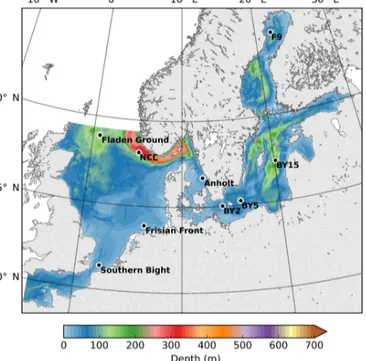
The model domain of Nemo-Nordic covers the English Channel, the North Sea and the Baltic Sea (Fig. 1). This domain bears similarities with that used in the NEMO-based configuration described by Maraldi et al. (2013). The resolution of the configuration of Maraldi et al. (2013) is higher than that of Nemo-Nordic but also uses the features of the NEMO ocean engine to build regional and coastal configurations. The main interest of the two configurations is different:

that of Maraldi et al. (2013) aims at resolving the European shelf dynamics, whereas the purpose of Nemo-Nordic is to represent the interaction between two basins with different dynamical features.

The area of Nemo-Nordic reaches from 4.15278^◦W to 30.1802^◦E and 48.4917–65.8914^◦N. The grid is geograph- ical, and in its 2 nautical mile version, the horizontal grid has zonal/meridional increments of 0.05^◦, which corresponds to a horizontal resolution of approximately 2 nautical miles (3704 m). The resolutions of approximately 1 or 2 nautical miles are given as approximations, especially at these high latitudes where zonal-scale factors differ between the southern and northern parts of the domain.

This resolution does not permit a proper description of the Danish Straits, which is a critical area of this configuration. However, in order to ensure a proper communication between the Baltic and the North Sea, we tune a proper

“impedance” of the Danish Straits in the model so that the flow between the two areas is consistent. We never checked if this feature allows a proper representation of the baroclinic flow within the straits, but since major Baltic inflows are mostly barotropic events we believe this is of secondary im-

(4)

Figure 1.The model domain and bathymetry of Nemo-Nordic. The filled circles show the locations of validation stations for salinity and temperature.

portance. However, a higher resolution of the Danish Straits will be implemented in the future using the AGRIF tool.

Nemo-Nordic usesz^∗vertical coordinates, which is more simple than some other Baltic Sea models such as Gräwe et al. (2015a) or the configurations developed by Shapiro et al. (2013). Advanced hybrid coordinates permit a better representation of dense overflows to the Baltic Sea but have a higher computational cost. However, the salinity biases based on the latest advances made in Nemo-Nordic show a very acceptable range, as shown in Sect. 4, and the benefit of z^∗ coordinates from a vertical point of view allow mul- tiple long-term simulations with realistic computing power.

Our model set-up comprises 56 vertical levels. The vertical resolution is adapted to the physical properties of the Baltic and North seas: the upper levels have a thickness of approximately 3 m until the typical level of the halocline is reached at 60 m. Below 60 m the layer thickness increases substan- tially: the layer thickness is 10 m at a 100 m depth, which is the typical halocline depth of the Norwegian Coastal Current (hereafter NCC) (Skagseth et al., 2011). Maximum values of 22 m are reached below 200 m. Note that the maximum decrease in resolution between two consecutive vertical levels is below 11 %. With these increments, the vertical resolution of Nemo-Nordic is adapted to Baltic Sea conditions and less optimal for resolving the halocline of the NCC. How- ever, the NCC is a baroclinic Kelvin wave which has a permanent renewal of stratification coming from the constant runoff flux of the Baltic Sea and all the river inputs located along the western Swedish and Norwegian coasts. Thus the

NCC halocline is less sensitive to coarse vertical resolution than the halocline of the Baltic Sea, which is not permanently renewed and is suspected of introducing spurious saltwater inflows into ocean models. Partial steps are used at bottom level to ensure a proper fit between the input bathymetry and the vertical grid.

The cross-sectional area of the Danish Straits is critical as it ensures the exchange between Baltic and North seas.

The resolution of the model does not permit having a proper representation of the Danish Straits. However, it is possible to represent each cross section so that it has the same hydraulic impedance as in reality. This was achieved by fitting the area of each critical cross section of the model with its equivalent area in the real world. More precisely, this means that the area of each critical “numerical cross section” of the model is made to fit with the surface of the real cross sections of the Danish Straits.

2.2 Physical settings

2.2.1 Free surface and time stepping

Nemo-Nordic uses a non-linear free surface (key_vvl) with a (key_dynspg_ts) option to split the computation of barotropic and baroclinic modes. In comparisons with previous ocean models such as that used by Meier (2004), which used a linear free surface, these features enable Nemo- Nordic to run in regions of high tidal amplitude like the North Sea and the English Channel. Tuning is done in order to obtain an accurate SSH representation. We use a variable bottom roughness (ln_bfr2d = .true.) along the cyclonic pathway of barotropic Kelvin waves in the North Sea.

This roughness is optimized to obtain the best possible SSH amplitude. Nemo-Nordic runs with a baroclinic time step of 360 s, which proved to be the best compromise between stability and computational speed. The barotropic time step is set to be 30 times smaller.

2.2.2 Mixing and dense overflows representation Vertical and horizontal mixing (and the connections between them) is a critical element when it comes to a Baltic and North Sea configuration. The major difficulty is to simulate the crucial dense water overflows in the Baltic Sea (Hordoir et al., 2015). In order to ease this process, Nemo-Nordic uses a bottom boundary layer parametrization (Beckmann and Döscher, 1997) for tracers (key_trabbl) in order to reduce the biases of a z coordinate ocean models when it comes to the representation of dense overflows. In NEMO, the bottom boundary layer can be used with an upstream ad- vection scheme or with a purely diffusive scheme or with a mixture of both. For Nemo-Nordic, sensitivity experiments have shown that the use of a purely diffusive scheme results in more realistic deep salinity in the Baltic Sea. Using an ad- vective scheme results in a lower deep salinity, most likely

(5)

due to a higher entrainment rate during major Baltic inflow events. One could object rightly that using sigma coordinates could have solved this issue without the use of such a parameterization. But using such a coordinate system would, on the other hand, create a strong diapycnal mixing of the Baltic Sea halocline and most likely pressure gradient errors in the steepest places of the North Sea such as the Norwegian trench.

However, the use of the bottom boundary layer parametrization is not enough to achieve a correct representation of the overflows. The tuning of the mixing was a major issue and required a tuning process. Nemo-Nordic includes two basins which have very different dynamical features: the North Sea is strongly influenced by tides, tidal mixing and relatively strong winds. In the North Sea, the stratification is relatively weak, with the exception of a summer thermocline in some regions, regions of freshwater influence (Simpson and Souza, 1995) and the region of the Norwegian Coastal Current (Hordoir et al., 2013). In contrast, the Baltic Sea has almost no tides, is less exposed to wind forcing and has a strong permanent stratification. Nemo-Nordic uses a two-equation turbulence closure, based on ak−turbulence scheme (key_zdfgls). In addition, the Galperin parameterization is used (Galperin et al., 1988), in order to preserve the Baltic Sea permanent stratification. This parameterization limits the mixing length computed by the vertical turbulence model in case of low turbulence and high stratification, which fits perfectly with the Baltic Sea halocline environment. This parameterization can be written following Eq. (1), in whichk is turbulent kinetic energy,N is the Brun–Väisälä frequency, andCgalpis the Galperin coefficient. Finally,lmaxis the maximum mixing length.

lmax=Cgalp

√ 2k

N (1)

Experiments done on the configuration without this latest parameterization yield a Baltic Sea permanent halocline that vanishes in a few years only. The Galperin coefficient is set to 0.17, which proves to be a good compromise between deep salinity and seasonal thermal stratification. A Galperin coefficient that is too high produces a higher deep salinity but also a very thin and unrealistic seasonal thermocline. In addition to the Galperin parameterization, the background levels of turbulent kinetic energy are turned to their minimum values, the goal being always to limit as much as possible mixing at the level of the Baltic Sea halocline.

Horizontal mixing is based on a Laplacian approach combined with the rotation of the horizontal diffusion tensor (key_ldfslp). However, this does not result in a real isopycnal diffusion in the sense that Nemo-Nordic is still based on a z coordinate system and not on isopycnal coordinates. Close to the bottom, sensitivity experiments have demonstrated that the rotation of the diffusion tensor did not enable us to follow dense salt inflows: increasing horizontal diffusivity resulted in lower deep salinity or even no pene-

tration of dense inflows at all, showing that diapycnal mixing is created by horizontal diffusion, even when the rotation of the diffusion tensor is activated. The first versions of Nemo-Nordic used a Smagorinsky approach in order to limit horizontal mixing as much as possible, but this approach finally resulted in very weak Baltic Sea salt inflows and a diffusivity impossible to control. Our final strategy has therefore been to create a viscosity/diffusivity coefficient which is high where model stability requires it the most (i.e. above the halocline), and low where it is crucial for diffusivity to be as low as possible to avoid diapycnal mixing. After a suite of sensitivity runs we decided on using spatially vary- ing values for viscosity and diffusivity. From the surface to a depth of 30 m the viscosity is set to values ranging from 30 to 50 m²s⁻¹for the Baltic and the North Sea, respectively, while we set diffusivity to a 10th of this value. Below this depth the values of viscosity is reduced to 0.1 m²s⁻¹. The same increase was applied to the diffusivity, which is still set to a 10th of the value for viscosity. This feature works as long as the Baltic Sea halocline is located at this precise depth but should be changed if the halocline depth changes. Along the open boundaries, the viscosity is increased to 800 m²s⁻¹ over the entire water column, decreasing rapidly to standard values within a few grid points inside the domain. This value is huge but prevented the model from ever crashing at the open boundary conditions. Several values were tried, and they proved to have little effect on the sea level variability inside the model domain.

A free slip option is taken for the lateral boundary conditions.

2.3 Boundary conditions 2.3.1 Open boundaries

Nemo-Nordic has two open boundaries: a meridional one in the western part of the English Channel and a zonal one set between Scotland and Norway. The setting of the boundary conditions uses the open boundary condition module of NEMO (key_bdy), as well as the tide module (key_tide).

Several settings can be used for boundary conditions. Tidal harmonics are taken from Egbert and Erofeeva (2002) and Egbert et al. (1994) although further investigation is also being made using the FES tidal model (Lyard et al., 2006).

Harmonical values for SSH are interpolated on the open boundaries of Nemo-Nordic. Harmonical tidal transports (in m²s⁻¹) are also interpolated in the same manner and then divided by the local depth of the Nemo-Nordic domain. In research mode, temperature and salinity boundary conditions may come from climatological data or from climate simulations, and a simple storm surge model is used. The model itself is corrected by a global ORCA0.25 configuration to take into account seasonal variability due to temperature and salinity variations. In operational mode, Nemo-Nordic uses

(6)

ECMWF forecast data for its SSH, temperature and salinity boundary conditions.

2.3.2 Atmospheric forcing

Nemo-Nordic has been so far used in forced mode using pre- scribed atmospheric conditions and the CORE bulk formula- tion (Large and Yeager, 2009).

To cover a long period, the atmospheric forcing is based on different sources. The driving data of the period 1961–1978 are based on downscaled ERA40 data (Uppala et al., 2005).

The ERA40 reanalysis is downscaled with the Rossby Centre regional atmospheric model version 4 (RCA4) with spectral nudging (Berg et al., 2013). The downscaling is necessary to improve the horizontal resolution of the global reanalysis data set. Here, we use data from an RCA4 set-up with a horizontal resolution of 11 km. The frequency of the driving data is hourly.

With the beginning of 1979 we change the atmospheric forcing to the SMHI reanalysis product EURO4M which is available until the end of 2013 (Dahlgren et al., 2016;

Landelius et al., 2016). The EURO4M data are available 3- hourly and with a horizontal resolution of 22 km. EURO4M incorporates data assimilation which ensures the best quality for our driving data. In operational mode (Nemo-Nordic 1 nm), the simulations were forced by HIRLAM C11 (http:

//hirlam.org, last access: 17 January 2019).

In forecast mode, Nemo-Nordic uses a combination of hourly ECMWF LL01 (9 km) data and Arome data (2.5 km).

2.3.3 Light penetration

A proper light penetration parameterization proved to be an important feature in order to reproduce the proper thermal structure, and especially the formation of a summer “Cold Intermediate Layer”. The Baltic Sea has turbid waters which prevent deep light penetration, concentrating the summer heat input close to the surface, and hence easing autumn cooling. Nemo-Nordic uses a red–green–blue light penetration parameterization, together with a constant chlorophyll value of 0.5 mg m⁻³to represent the turbid Baltic Seawaters.

Failing to use chlorophyll concentration results in a cold intermediate layer that is too thin and too shallow. This chlorophyll concentration does not pretend to be realistic from a biogeochemical point of view, it corresponds to a mean value for both basins which allows a realistic light penetration in an area which has a water turbidity higher than that of the global ocean.

2.3.4 River discharge

The Baltic Sea salinity is sensitive to the accumulated freshwater input since the exchange with the open ocean is very limited (e.g. Meier and Kauker, 2003). Freshwater supply to the Baltic Sea in the simulation must therefore be han- dled with care. Here, we are using data from the HYdrolog-

ical Predictions for the Environment (HYPE) model (Don- nelly et al., 2016). The model simulates a mean runoff to the Baltic Sea of roughly 16 000 m³s⁻¹for the period 1981–

1998. However, Meier and Kauker (2003) state that the observed runoff for the same period is 15 053 m³s⁻¹with an even lower value (14 085 m³s⁻¹) for the period 1902–1998.

Consequently, we reduced the freshwater supply computed by HYPE. We have chosen a general reduction of 10 % which gives more realistic runoff for the Baltic Sea. Moreover, this improved the Baltic Sea salinity (not shown). The freshwater input to the North Sea including the Skagerrak and Kat- tegat area amounts to 11 515 m³s⁻¹ after the reduction by 10 %. The river runoff is spread over 424 river mouths in the entire model domain whereas more than 250 are located in the Baltic Sea (excluding the Skagerrak and Kattegat area).

The UNESCO equation of state for seawater is used. The reference density is set to 1035 kg m⁻³, which is most likely overestimated. Further experiments should be done on this point.

2.3.5 Sea ice

Nemo-Nordic benefits from the use of the NEMO ocean engine and of its advanced sea ice model LIM3. Sea ice is a feature specific to the Baltic Sea that is due to the Baltic Sea’s low salinity. Being able to represent sea ice dynamics properly is compulsory when it comes to a Baltic Sea ocean model. Models such as Gräwe et al. (2015a) do not include this feature. The sea ice in Nemo-Nordic is validated in Pemberton et al. (2017). Comparison done with Funkquist and Kleine (2007) suggest that Nemo-Nordic so far reaches the highest accuracy of sea ice representation for the Baltic Sea.

3 Validation of barotropic mode and surface currents 3.1 Sea level

To model and forecast SSH is one of the major aims of Nemo-Nordic. This section provides a statistical comparison between measured and modelled SSH at different tide gauges in the Baltic and North seas.

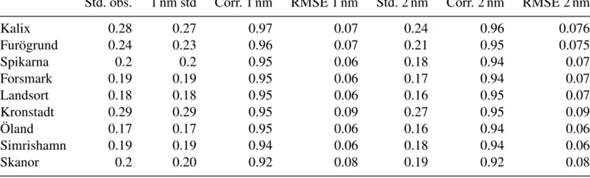
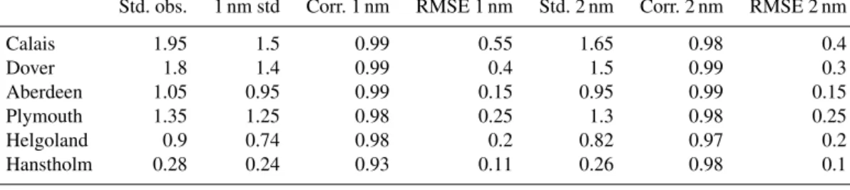
We have chosen tide gauges which are as representative as possible of three respective regions: the Baltic Sea (Ta- ble 1), the Danish Straits plus the Kattegat and the Skagerrak (Table 2), and the North Sea, including the English Channel (Table 3). The comparisons are based on an 18-month period, lasting from 1 July 2011 and ending on 31 December 2012, at an hourly frequency. The respective model simulation was started 1 month before to allow for a spin-up time. Each area is presented in a specific array.

There is generally a very high correlation between model and observations in almost all regions. In the North Sea and the English Channel, correlations are highest and mostly close to 0.99, with the one exception of Hanstholm, where

(7)

Table 1.SSH representation, in terms of correlation, standard deviation (metres) and root-mean-square deviation (metres), made by Nemo- Nordic for nine Baltic Sea stations. The comparison is based on an 18-month period, starting on 1 July 2011, and on hourly output SSH.

Std. obs. 1 nm std Corr. 1 nm RMSE 1 nm Std. 2 nm Corr. 2 nm RMSE 2 nm

Kalix 0.28 0.27 0.97 0.07 0.24 0.96 0.076

Furögrund 0.24 0.23 0.96 0.07 0.21 0.95 0.075

Spikarna 0.2 0.2 0.95 0.06 0.18 0.94 0.07

Forsmark 0.19 0.19 0.95 0.06 0.17 0.94 0.07

Landsort 0.18 0.18 0.95 0.06 0.16 0.95 0.07

Kronstadt 0.29 0.29 0.95 0.09 0.27 0.95 0.09

Öland 0.17 0.17 0.95 0.06 0.16 0.94 0.06

Simrishamn 0.19 0.19 0.94 0.06 0.18 0.94 0.06

Skanor 0.2 0.20 0.92 0.08 0.19 0.92 0.08

Table 2.SSH representation, in terms of correlation, standard deviation (metres) and root-mean-square deviation (metres), made by Nemo- Nordic for nine stations located in the Danish Straits, the Kattegat and the Skaggerak. The comparison is based on an 18-month period, starting on 1 July 2011, and on hourly output SSH.

Gedser 0.23 0.21 0.93 0.08 0.21 0.94 0.08

Barsebäck 0.18 0.19 0.88 0.09 0.14 0.68 0.13

Klagshamn 0.18 0.18 0.91 0.08 0.19 0.92 0.08

Rödvig 0.21 0.2 0.93 0.08 0.19 0.92 0.08

Göteborg 0.22 0.21 0.91 0.09 0.18 0.93 0.08

Smögen 0.22 0.23 0.91 0.1 0.2 0.93 0.08

Viken 0.21 0.19 0.90 0.1 0.18 0.90 0.1

Skagen 0.24 0.26 0.90 0.11 0.225 0.91 0.1

Kungsvik 0.24 0.25 0.92 0.1 0.22 0.93 0.09

correlations are around 0.93. In the Baltic Sea, correlations are always close to 0.95. In the narrow Danish Straits and the Kattegat, regions with complicated topography, the correlations are lowest, but still generally exceed 0.9. Exceptionally low correlations (0.68) are obtained in Barseback and only when Nemo-Nordic 2 nm is used. When Nemo-Nordic 1 nm is used, the minimum depth of the ocean model is set to 3 m, compared to 9 m, which gives a better representation of the shallow banks located in the Öresund area and of the am- plification of barotropic waves. This feature was not implemented in Nemo-Nordic 2 nm where the main focus is the Baltic–North Sea exchange. Using wetting and drying in the future should help better representations of SSH in shallow areas affected by strong sea level variability.

Biases in terms of SSH representation can be summarized as follows. Nemo-Nordic usually has a negative bias in terms of the representation of the low frequencies in the North Sea, the Skagerrak and the Kattegat. In the same regions, the opposite bias may be noticed when it comes to higher frequencies: tidally driven SSH can present overshoots in some places. In the Baltic Sea, one may notice that the tidal sig- nal is usually a bit too high, but since its amplitude remains very small in comparison to other frequencies, it does not affect the quality of the SSH representation significantly. The

representation of lower frequencies does not reveal any sig- nificant bias in the Baltic Sea.

Nemo-Nordic 1 nm represents SSH better than Nemo- Nordic 2 nm, which is partially due to the higher resolution for most features. For example, in the Danish Straits, the representation of shallow banks has been taken into account in Nemo-Nordic 1 nm, and the size of the cross sections has been adapted to represent the North Sea–Baltic Sea exchange. This allows us to amplify incoming barotropic waves, which is essential in order to get the right SSH variability in the Danish Straits tide gauges. In Nemo-Nordic 2 nm, the main concern has been to ensure the correct Baltic–

North Sea exchange, which is crucial for having a correct representation of Baltic Sea salt inflows, which are one of the main drivers of the Baltic Sea ecosystem and of its long-term thermo-haline structure.

In summary, we identified the following key processes to model realistic SSH variations.

– In Nemo-Nordic, the SSH and SSH variability in the North Sea is to a first order barotropicaly driven and is built by a combination of tidal waves entering through the northern boundary and western boundaries, wind- driven SSH built over the North Atlantic, and wind- driven SSH over the North Sea. To get a correct rep-

(8)

Table 3.SSH representation, in terms of correlation, standard deviation (metres) and root-mean-square deviation (metres), made by Nemo- Nordic for six stations located in the North Sea. The comparison is based on an 18-month period, starting on 1 July 2011, and on hourly output SSH.

Calais 1.95 1.5 0.99 0.55 1.65 0.98 0.4

Dover 1.8 1.4 0.99 0.4 1.5 0.99 0.3

Aberdeen 1.05 0.95 0.99 0.15 0.95 0.99 0.15

Plymouth 1.35 1.25 0.98 0.25 1.3 0.98 0.25

Helgoland 0.9 0.74 0.98 0.2 0.82 0.97 0.2

Hanstholm 0.28 0.24 0.93 0.11 0.26 0.98 0.1

resentation of the SSH variability and the cyclonic circulation in the North Sea, it is important to have high- frequency (hourly) boundary conditions that take into account all these aspects.

– In the Kattegat–Skagerrak region, as one moves further towards the entrance of the Baltic Sea, the effect of tides and of high-frequency waves generated in the North At- lantic or the North Sea becomes less important. The low frequencies, on the other hand, generated by the storm surge model over the North Atlantic turned out to be important for this region. The shelf break along the coast amplifies the effect of coasts on barotropic waves arriving from the North Sea and helps representing SSH variability and its extremes. A higher vertical resolution in the shallow areas improves the representation of the SSH variability, especially in the Skagerrak–Kattegat.

This last effect becomes crucial in the Danish Straits where the shallow banks need to be represented.

– The SSH variability in the Baltic Sea is barely influenced by any tidal variability but is highly influenced by low-frequency forcing coming from the North At- lantic and the North Sea. In addition, local wind forcing over the Baltic Sea explains higher frequencies. The only communication between the Baltic and the North Sea being the Danish Straits, the adjustment of cross sections and of the friction in this area are of crucial im- portance to chose which barotropic frequencies can penetrate the Baltic Sea. The Danish Straits should act as a well-tuned low-pass filter which allows low-frequency waves to penetrate the Baltic Sea but lets little high- frequency power enter the Baltic Sea.

3.2 Surface currents 3.2.1 General circulation

The model reproduces the general cyclonic surface circulation pattern in the North Sea (OSPAR, 2000), with a southward flow in the western part of the basin, a northeastward flow along the southern coast and a northward flow along the Norwegian coast in the Norwegian Coastal Current (Fig. 2).

The strongest modelled southward flow of Atlantic water through the northern boundary occurs just next to the NCC.

This flow forms a current that flows south-east and enters the well-known cyclonic circulation pattern in the Skager- rak, in good agreement with the observed surface currents in the North Sea (OSPAR, 2000). A part of the southward flow along the British Isles also deviates eastward to directly join the eastward flow towards the Skagerrak. Another part flows further to the south and mixes with inflow from the English Channel. The larger part of inflowing Atlantic water from the northern boundary is restricted to north of 54^◦N and then recirculates mainly following the topography of the Dogger Bank. The southern North Sea is dominated by inflow waters from the English Channel.

In the Baltic Sea and its sub-basins the model reproduces the observed general cyclonic circulation patterns (Elken and Matthäus, 2008), with a southward flow in its western part and a northward flow in its eastern part. In the Gotland basin the model reproduces the southward flow on both sides of Gotland and the northward flow along the coast of the Baltic, giving rise to the cyclonic structure over the Got- land Deep (Fig. 2). In the Kattegat the model simulates a general anticyclonic flow in agreement with Nielsen (2005) and resolves the northward flowing Baltic Current along the Swedish coast, which feeds low-saline waters into the NCC.

3.3 Overturning circulation

The inflows and outflows through critical cross sections, where observational estimates exist, have been calculated for the period 1979–2010. Inflows are defined as volume transports directed inwards to the domain, and outflows are defined as transports directed outwards. For the Baltic Sea a longitudinal cross section has been taken along 12.90^◦E, and inflowing waters are defined as transports in the positivex direction and outflows as those in the negative direction. For the Strait of Dover a longitudinal cross section has been taken along 50.99^◦N. Here the flow is barotropic and there is only a mean inflow to the North Sea. For the northern boundary, taken along 58.06^◦N, the inflow is all transports in the nega- tiveydirection and the outflow is all transports in the positive ydirection.

(9)

Figure 2. Simulated surface (0–30 m) currents; climatology for 1979–2010. The lines and arrows show the streamlines and direc- tions of the current vector field. The thickness of the line is scaled with respect to the speed of the current. The filled contours show the current speed in m s⁻¹.

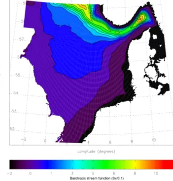
As shown in Table 4, the modelled transports agree well with observational estimates, which is an additional indica- tion that the general circulation of the North Sea and the Baltic Sea is reproduced well by the model. The modelled flows gives a water residence time of 23 and 1.8 years in the Baltic Sea and the North Sea, respectively.

The circulation in the North Sea is mainly of a barotropic feature. Barotropic stream functions of the horizontal overturning circulation, showing the general cyclonic circulation of the North Sea, are displayed in Fig. 3. The largest flows are found in the Norwegian trench, where the overturning barotropic circulation amounts to 0.9 Sv, in good agreement with the calculated fluxes in Table 4.

4 Salinity and temperature

4.1 Surface temperature and salinity

A validation of the simulated mean surface salinity and temperature is made (Figs. 4 and 5) using the Janssen et al.

(1999) climatology. The values are computed as a mean value over the first 10 m. For the Baltic and the North Sea, the overall surface salinity is reproduced well. There is, however, a positive surface bias in the Baltic Sea. One may notice, in particular, that the penetration of the 8 PSU iso-haline within the estuary is too high. The 7 PSU iso-haline is also located a few nautical miles too far north. In the North Sea there is a negative bias in freshwater-influenced areas (the NCC and in the southern German Bight). For sea surface temperature (SST), the structure is similar to observations but there is a positive bias of less than 1^◦over all the domain. This bias seems to partially come from a warm bias in the atmospheric

Figure 3.Barotropic stream function (Sv); climatology for 1979–

2010.

forcing (in winter) (Landelius et al., 2016) and partially from surface overshoots during the summer period. Sensitivity experiments have shown that the positive SST bias during summer time is lower if the Galperin coefficient used to main- tain a stable haline stratification is lowered. In order to avoid these effects, further development is being made to decouple the Galperin parameterization from thermal effects.

4.2 Thermohaline structure of the Baltic Sea

The thermohaline structure of the Baltic Sea exhibits two types of variability. First, a spatial variability which leads to the Baltic Sea having strong salinity gradients from the surface to the bottom but also presents estuarine features which result in a decreasing salinity from south to north. Strong temperature gradients also exist as the northern regions of the Baltic Sea have a much colder climate than those located in its southern part. From a temporal point of view, surface salinity exhibits a seasonal variability (Hordoir and Meier, 2010), and deep salinity has a lower variability highly related to the occurrence of deep salt inflows (Hordoir et al., 2015).

Surface temperature has a strong seasonal cycle related to summer stratification and its destruction during autumn. The model’s ability to reproduce the thermohaline structure and its variability on different timescales will be validated below.

4.2.1 Vertical structure and seasonal variability The haline vertical structure of the Baltic Sea is in general reproduced well by Nemo-Nordic (Fig. 6), with a distinct halocline separating the surface waters from the deeper waters.

(10)

Table 4.Volume flow (Sv) through cross sections; climatological mean for 1979–2010.

Model Observations

Cross section Inflow Outflow Inflow Outflow Reference

Strait of Dover 0.110 – 0.11–0.17 – Otto et al. (1990), and references therein Northern boundary 0.794 0.928 0.93–1.73 1.34–1.8 Otto et al. (1990), and references therein

Baltic Sea 0.029 0.044 0.027 0.043 Savchuk (2005)

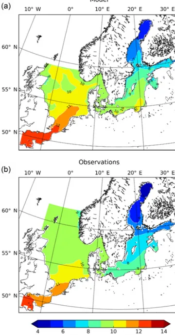
Figure 4.Mean surface (0–10 m) salinity for the Baltic, North Sea and English Channel, as simulated by Nemo-Nordic for the period 1979–2010 (a) and from observations (b) from Janssen et al. (1999).

Figure 5.Mean surface (0–10 m) temperature for the Baltic, North Sea and English Channel, as simulated by Nemo-Nordic for the period 1979–2010(a)and from observations(b)from Janssen et al.

(1999).

(11)

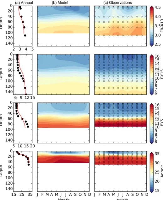
Figure 6.Haline structure of four different stations of the Baltic Sea from top to bottom: F9-A13 station in the Bothnian Bay, BY14 station in the Baltic proper, BY5 station in the Bornholm Basin and Anholt station in the Kattegat. Column(a)displays annual mean depth profiles, where the red line is simulated salinity and black dots are observations. Columns(b)and(c)show seasonal variations in the model and the observations, respectively. In column(c), the transparent circles show sample depths; the observations are based on a 1979–2010 climatology.

In the Bothnian Bay and the Kattegat (F9-A13 and Anholt), the modelled depth (50 and 20 m, respectively) and strength of the halocline correspond well to observations. There is a small negative salinity bias over the whole water column in the Bothnian Bay, while the overall salinity is reproduced well in the Kattegat. In the Baltic proper and the Bornholm Basin (BY15 and BY5), the modelled halocline is weaker and shallower than the observed one. The surface water at these stations tends to have a positive bias, while the deeper waters tend to have a negative bias, suggesting too strong a mixing between surface and deep waters. No stronger sea-

sonal cycles exist in the haline structure, except for a freshwater pulse arriving in the surface waters during summer months, which is captured by the model at all stations.

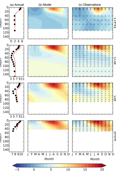
The thermal vertical structure is dominated by the seasonal thermocline. In the Kattegat, Bornholm Basin and the Baltic proper (Anholt, BY5 and BY15), it starts forming earlier than in the Bothnian Bay (F9-A13), both in the model and in the observations (Fig. 7). The later formation of the thermocline in the Bothnian Bay is partially due to the lower insolation at higher latitudes but also due to the non-linearity of the equation of state at low salinities. The temperature of max-

(12)

Figure 7.Thermal structure of four different stations of the Baltic Sea from top to bottom: F9-A13 station in the Bothnian Bay, BY14 station in the Baltic proper, BY5 station in the Bornholm Basin and Anholt station in the Kattegat. Column(a)displays annual mean depth profiles, where the red line is simulated temperature and black dots are observations. Columns(b)and(c)show seasonal variations in the model and the observations, respectively. In(c)the transparent circles show sample depths; the observations are based on a 1979–2010 climatology.

imum density is higher at lower salinities, meaning that the water column has to completely mix before the formation of the thermocline can start, which is reproduced well by the model. The model’s development of the seasonal thermocline and its deepening agrees well with observations in the Kattegat, the Bornholm Basin and in the Baltic proper.

In the Bothnian Bay no conclusions can be drawn on this as- pect due to a lack of measurements between 15 and 40 m, where the thermocline is situated. The break-up of the ther-

mocline is also well represented in the model. The model has, on the other hand, difficulties in representing the colder intermediate waters in the Bornholm Basin and the Baltic proper, which have a warm bias. This might be related to biases in the atmospheric forcing (Landelius et al., 2016), as these waters are formed during winter convection. Indeed, the simulated winter surface temperatures at BY5 and BY15 tend to have a warm bias. The modelled cold intermediate waters also descend too deep towards the end of the year.

(13)

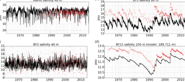
Figure 8.Time series of modelled salinity (black) and observations (red) for different stations. The stations are, from top to bottom, Anholt, BY2, BY5 and BY15 (see Fig. 1 for their location). All stations are relevant for inflowing salty water masses from the North Sea to the Baltic Sea. The chosen levels are all close to the bottom of the corresponding location.

This might be related to the weaker halocline, and thus probably stronger mixing, in the model. The deep waters below the halocline are warmer than the intermediate waters, which is reproduced by the model. In the model it is, however, about 0.5^◦warmer than in the observations at the BY15 station.

4.2.2 Interannual variability

From the comparison between the observations and their variability (Fig. 8), one notices that Nemo-Nordic in general reproduces the variability in the deep-water salinity close to the bottom well, both in the Kattegat and in the Baltic Sea, despite the constant background bias in the salinity. Espe- cially, it is interesting to note from the BY15 salinity that the model is able to reproduce the major Baltic inflows of 1993 and 2003. The mechanisms behind the major Baltic inflows are actually mostly barotropic, although their propa- gation to the bottom of the Baltic Sea involves mixing processes. Therefore, the representation of sea level variability is a key element in reproducing the variability in the major Baltic inflows. A comparison of the modelled and measured sea level differences during the recorded durations of these inflows shows the model’s accuracy to represent the under- lying barotropic processes. During the duration of the 1993 major Baltic inflow, the sea level at Landsort increases by 1 m in observations against 1.02 m in the model, while during the 2003 major Baltic inflow, the sea level at Landsort increases by 0.58 m both in the model and in the observations. This further suggests that a misrepresented baroclinic process must be responsible for the negative bias in deep-water salinity in the Baltic Sea. Even though this model uses a bottom boundary layer parameterization (Beckmann and Döscher, 1997), it is still azcoordinate model, which means that the representation of dense overflows is not as accurate as it would be

in a sigma or generalized vertical coordinate model. It is also interesting to note that Nemo-Nordic tends to overestimate the variability in deep-water salinity at the Anholt station in the Kattegat, while it slightly underestimates the variability at the BY2 station.

4.2.3 Short-term variability – comparison with Argo floats data

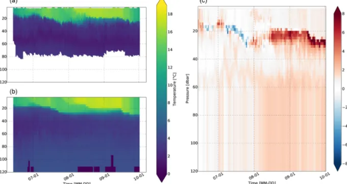
As an example of Nemo-Nordic’s performance in the shorter term, we compared the model results to temperature observations from an autonomous Argo buoy. Over 100 profiles were collected during a mission in the Bothnian Sea, which lasted from 13 June to 2 October 2013. The profiles were taken from between 61.57 and 62.47^◦N in latitude and between 19.59 and 20.42^◦E in longitude. This data set has been described in detail by Westerlund and Tuomi (2016), who also provided an illustration of the buoy route. From a comparison of observed and modelled temperature profiles we see that the seasonal thermocline is visible throughout the summer (Fig. 9). The vertical structure of temperature was relatively reproduced well by Nemo-Nordic near the surface.

In August the thermocline reached maximum depth and temperature. The model was able to describe well how the mixed layer deepened during the summer. The temperature gradient of the thermocline was also well represented. The surface layer responded to atmospheric forcing in a similar way in observations and model. In layers under the thermocline, model temperatures were somewhat too high. This bias increased in late summer. Deeper, the dicothermal (old winter water) layer was not as pronounced in the model as it was in the observations. In late August, the model predicted larger thermocline depths than were observed. In general, temperature profiles were smoother in the model than in observa-

(14)

Figure 9.Comparison of temperature profiles from an Argo float(a)and Nemo-Nordic(b). Observational data in(a)have been redrawn from the data set used by Westerlund and Tuomi (2016). Panel(c)shows the difference between the observation and model run. The model was larger than the measurement where the difference is positive. Model results have been taken along the buoy route in the Bothnian Sea in 2013.

tions. Furthermore, some finer-scale features were not completely reproduced by the model.

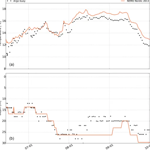
Observed and modelled near-surface temperatures, along with estimated thermocline depths, are shown in Fig. 10.

Near-surface temperature was taken to be the temperature of the model point at the depth of the topmost data point in the observations, which was typically around 4 m, depending on the profile. In most cases this is very close to the surface temperature. The location of the thermocline was taken as the place of the maximum temperature gradient along thezaxis.

Near-surface temperature in the model overall reproduced the seasonal temperature cycle, although in early September surface temperatures were around 1^◦ greater in the model than in observations. Thermocline depths were represented quite well in the model, except for the aforementioned time in late August. Westerlund and Tuomi (2016) presented a similar comparison to a different model configuration, derived from an earlier version of Nemo-Nordic. That model used different atmospheric forcing fields taken from an operational HIRLAM forecast from the FMI (Finnish Meteo- rological Institute), climatological boundary conditions, climatological river runoffs and initial conditions from FMI’s operational Baltic Sea forecast. Furthermore, it did not have the light penetration parameterization present in the official Nemo-Nordic configuration described in this paper. Com- pared to those results, the near-surface temperature in the official Nemo-Nordic results differs more from the observa-

tions in autumn but shows less bias in early summer. Ther- mocline depths were quite similar in both configurations.

4.3 Thermohaline structure of the North Sea

Compared to the Baltic Sea, the North Sea is more homogeneous regarding its thermohaline structure. It exhibits mostly seasonal variations in the form of the formation of the seasonal thermocline and seasonal variations in freshwater forcing. Haline fronts between coastal and offshore areas are found in the southern and eastern North Sea due to the relatively large river runoff from continental rivers at the southern shore of the North Sea and the Norwegian Coastal Cur- rent carrying low-saline waters from the Baltic Sea.

4.3.1 Vertical structure and seasonal variability In this section we validate the vertical structure and seasonal variability at four stations representative of different hydrological regimes in the North Sea. Two stations are located near the boundaries towards the Atlantic Ocean (Fladen Ground and the Southern Bight). Validating the temperature and salinity structure in these areas also gives a validation of the boundary conditions and the properties of the inflowing water. The open boundary condition fields for tracers (T and S) come from a climatology in this case, so it is interesting to check whether their use with the model enables it to represent measurements. The two other stations (NCC and Frisian Front) are located in areas where there are relatively large

(15)

Figure 10.Near-surface temperature in 2013 from the Argo float data and from Nemo-Nordic. Thermocline depth estimated as the maximum of vertical temperature gradient in panel(b).

horizontal and vertical (only NCC) salinity gradients due to the freshwater forcing from the Baltic Sea and the continental rivers draining into the southern North Sea. The observational data comes from the KLIWAS data set provided by the University of Hamburg (Bersch et al., 2013). It is composed of all available measurements between 1970 and 2013 in the North Sea, which have been put into a 1×1 grid.

The haline vertical structure at the four stations in the North Sea is displayed in Fig. 11. The only station with a distinct permanent haline stratification is the NCC station.

The vertical haline structure at this station is reproduced well by the model, although the surface waters are less saline than the observations by about 1 PSU. The other stations are rather homogeneous in the vertical with respect to salinity. In the Southern Bight and the Fladen Ground, the model captures the overall mean salinity. At the Frisian Front the modelled salinity is about 1.5 PSU too low, which is probably related to a displacement of the front between coastal waters with lower salinity and offshore waters. At all stations the model simulates a seasonal cycle in the surface salinity with a freshening during the summer months, in agreement with the observa-

tions. The timing and the amplitude of this summer freshening is, however, subject to some biases. Because the data set does not contain regular measurements from these positions it can, on the other hand, give rise to biases in the observational estimates of the seasonal cycle.

The thermal vertical and seasonal structure is, as for the Baltic Sea, dominated by the seasonal warming and cooling of the surface waters (Fig. 12). In the Southern Bight and at the Frisian Front the waters are well mixed from surface to bottom throughout the year, and no seasonal thermocline develops, which is reproduced well by the model. In the South- ern Bight there is a warm bias of the order of 0.5^◦C (annual mean) in the model throughout the water column. At the Frisian Front there is a warm bias of about 0.3^◦C in the surface waters. At the two deeper stations, the seasonal development and the depth of the thermocline are reproduced well in the model, although the start of the thermocline formation is somewhat too early in the model. This is the case especially at the Fladen Ground, where it starts almost 1 month too early. Also the winter SSTs are too warm in the model, resulting in too weak a winter convection or temperatures

(16)

Figure 11.Haline structure of four different stations of the North Sea from top to bottom: Southern Bight station, Frisian Front station, NCC station and Fladen Ground station. Column(a)displays annual mean depth profiles, where the red line is simulated salinity and black dots are observations. Columns(b)and(c)show seasonal variations in the model and the observations, respectively. The observations are based on a 1979–2010 climatology.

of the convecting water that are too warm, which in its turn gives a warm bias in the deep waters. At both stations there is a warm bias of about 0.5^◦C (annual mean) in the surface waters.

4.3.2 Modelled thermocline dynamics

For biogeochemical processes summer thermal conditions are important when water temperature and light intensity stimulate the growth of phytoplankton. Contemporaneously, thermal stratification develops in the deeper basin of the northern North Sea and the inflow of Atlantic water weakens (Skogen et al., 2011); accordingly atmospheric forcing

at the surface becomes more important. This leads to sub- stantially better reproduction of interannual variability even in the north (Fig. 14b). We analyse in the following the modelled thermocline dynamics following previous approaches for the North Sea (Pohlmann, 1996; Meyer et al., 2011;

Mathis and Pohlmann, 2014), which define the presence of thermocline conditions when a certain vertical temperature gradient is exceeded. We here chose a critical gradient of 0.25^◦C m⁻¹. The yearly maximum extent of stratified areas is primarily governed by topography and wind stress (Mathis and Pohlmann, 2014) and varies between 100 000 and 185 000 km²in 1990 and 2005. Stratified conditions be-

(17)

Figure 12.Thermal structure of four different stations of the North Sea from top to bottom: Southern Bight station, Frisian Front station, NCC station and Fladen Ground station. Column(a)displays annual mean depth profiles, where the red line is simulated temperature and black dots are observations. Columns(b)and(c)show seasonal variations in the model and the observations, respectively. The observations are based on a 1979–2010 climatology.

gin to develop in May and reach their maximal intensity during July and August. Already during September wind stress strengthens and temperatures lower, which increases mixing.

The thermocline weakens then and is shifted downward. As a result, nutrient-rich water reaches the euphotic zone. During this time, a second phytoplankton bloom can be sometimes observed in the North Sea (van Haren et al., 2003; Moll, 1998).

4.3.3 Interannual variability

Surface properties are in many cases dominated by local meteorological forcing (Skogen et al., 2011). Therefore, it is important to also validate subsurface properties, which are also influenced also the by circulation dynamics (like Atlantic inflow). For this, we use the KLIWAS observational data set (Bersch et al., 2013). We here follow previous approaches and subdivide the North Sea into 1^◦×1^◦boxes for which for each month and at each box, standard level Taylor statistics

(18)

Figure 13. Seasonal cycle of thermocline structure.(a)Thermocline intensity (^◦C m⁻¹) averaged over the entire thermal stratified area.

(b)Same as in(a)but for thermocline depth (m).

Table 5.Quantitative comparison of simulated and observed state variables derived from Taylor statistics (Taylor, 2001). Rms: root mean squared; corr: Pearson’s correlation; SD: standard deviation;N: number of observations. The statistics have been derived from all 1^◦×1^◦ boxes. See text for details about data set and data handling.

State variable rms corr SD observation SD simulation N Winter

Temperature 0.74 0.78 0.86 1.18 6139

Salinity 0.56 0.79 0.54 0.88 6034

Summer

Temperature 1.10 0.94 3.06 3.15 6808

Salinity 0.56 0.83 0.72 0.98 6638

(Taylor, 2001) are calculated (for details, see Raddach and Moll, 2006; Gröger et al., 2013). In order to estimate the interannual variability in seasonal signals, we chose January and July as representative of winter and summer as in these month observations were most abundant in the observational data set. The results are shown in Table 5. In total, 25 619 observations were used for the analysis.

Overall, good correlation with the temperature and salinity observations for summer and winter indicates the model’s skill to capture interannual variability and thus the ability to realistically respond to low-frequency modes of climate variations such as decadal variability or the NAO (North Atlantic Oscillation) which likely influence the North Sea hydrography (e.g. Hjøllo et al., 2009; Mathis et al., 2015). The root mean square values lie well within the standard deviation of the observations (with the exception of January salinities where rms is slightly higher; Table 5). The model’s salinity variability (as indicated by standard deviation) is too high (∼50 %), but the spatial distribution of the observations is much coarser than the model grid, which explains this result.

4.3.4 Comparison with satellite data

In the following we compare the modelled SST with a widely used satellite product provided by the Federal Maritime and Hydrographic Agency of Germany, Hamburg (Bundesamt für Seeschifffahrt und Hydrographie; hereafter BSH). By this we are able to investigate how the modelled SST reproduces interannual variability, which is important for the application of the model to climate services and the simulation of various climate scenarios.

In contrast to the warm bias relative to the in situ temperature measurements, the simulated winter SST (Fig. 14) is almost everywhere colder than the satellite estimations of SST. Cold biases relative to satellite measurements were also obtained in other ocean models driven by the ERA40 reanalysis data set in Tian et al. (2013) and Gröger et al. (2015).

Given that in situ temperature measurements give a more di- rect measure than satellite estimations of SSTs and that the atmospheric forcing used for these simulations has a warm bias, especially in the North Sea during winter (Landelius et al., 2016), it is likely that the satellite underestimates the SST. Despite this, the satellite SSTs can be used for validation of spatial and temporal variability.

(19)

Figure 14. (a)Left-hand panels: Nemo-Nordic multiyear (1990–2005) DJF average SST. Middle panels: Nemo-Nordic minus BSH SST.

Right-hand panels: Correlation between Nemo-Nordic SST and BSH SST. Note that regions where not enough observational data were present have been coloured grey. Panel(b)is same as(a)but for JJA.

Figure 14a shows an overall good correlation of modelled interannual SST variations with the BSH data set. Likewise the lower correlation in the northern deeper parts could indi- cate problems with convective and/or wind-induced mixing which would influence the heat transfer from the deeper layers to the surface. In contrast, in the southern and shallower parts, SSTs are dominated largely by the atmospheric forcing (Skogen et al., 2011), and thus correlation increases. Good correlation is also seen along the Norwegian coast where the effective heat capacity is limited due to haline stratification, which makes SSTs more sensitive to the atmospheric forcing. The same is true for nearly the entire Baltic Sea, where correlation drops below 0.8 almost nowhere.

5 Conclusions

In this article we provide a detailed description of the dynamic features of Nemo-Nordic, a newly developed joint set- up for the Baltic Sea and the North Sea. Its performance when it comes to sea ice is the subject of a specific article (Pemberton et al., 2017). We have shown that Nemo-Nordic is able to reproduce the barotropic and baroclinic dynamics, as well as the thermohaline structure, of Baltic and North Sea basins. The key to achieve this overall good representation of the physics in the Baltic Sea and the North Sea has been to get as good a representation of the barotropic dynamics as possible. This ability, which is detailed in the present article, has been validated with the most demanding procedure: Nemo- Nordic is used as the official forecast model of SMHI for the Baltic and North seas, including for SSH, for which the

model does not benefit of any data assimilation. In forecast mode, Nemo-Nordic is used with a higher resolution (1 nm or 1852 m), compared to longer integrations where the set-up is used with a 2 nm (or 3704 m) resolution. The ability of the model to represent barotropic dynamics at high-frequency timescales (hours to several days) is the main reason for its good representation of transports and water exchanges in and between the Baltic Sea and the North Sea. It also allows for an accurate representation of the Baltic Sea inflows and the initiation of the Baltic Sea baroclinic dynamics. In order for Nemo-Nordic to properly represent baroclinic dynamics in both basins, a specific tuning of mixing is done from both horizontal and vertical points of view. For example, a limita- tion of the vertical mixing length is needed in order to help the model keep the Baltic Sea halocline at a realistic level.

Although Nemo-Nordic reproduces the overall physics of Baltic and North Sea well, some biases may be noticed. The sea level representation is better in forecast mode than that of the previous SMHI operational model HIROMB, but some improvements are still needed to better represent extreme events. Regarding this precise point, a coupling with wind waves appears to be the next step, as it was recently shown that the contribution of wind waves has a major impact on extreme sea levels (Staneva et al., 2016). Ongoing development based on the new implementations within the NEMO ocean engine concerns the inclusion of wetting and drying processes, which can also affect sea level in shallow areas.

Further, an important margin of improvements exists in atmospheric forcing, bottom friction and bathymetry. A margin that should lead to an even greater accuracy in sea level rep-