Intergenerational Transmission of Unemployment - Causal Evidence from Austria

(1)

IHS Working Paper 14

April 2020

Intergenerational Transmission of Unemployment - Causal Evidence from Austria

Dominik Grübl

Mario Lackner

Rudolf Winter-Ebmer

(2)

Author(s)

Dominik Grübl, Mario Lackner, Rudolf Winter-Ebmer

Title

Intergenerational Transmission of Unemployment - Causal Evidence from Austria

Institut für Höhere Studien - Institute for Advanced Studies (IHS) Josefstädter Straße 39, A-1080 Wien

T +43 1 59991-0 F +43 1 59991-555 www.ihs.ac.at ZVR: 066207973

License

„Intergenerational Transmission of Unemployment - Causal Evidence from Austria“ by Dominik Grübl, Mario Lackner, Rudolf Winter-Ebmer is licensed under the Creative Commons: Attribution 4.0 License (http://creativecommons.org/licenses/by/4.0/) All contents are without guarantee. Any liability of the contributors of the IHS from the content of this work is excluded.

All IHS Working Papers are available online:

https://irihs.ihs.ac.at/view/ihs_series/ser=5Fihswps.html

This paper is available for download without charge at: https://irihs.ihs.ac.at/id/eprint/5286/

(3)

Intergenerational Transmission of Unemployment – Causal Evidence from Austria

^*

Dominik Gr¨ubl^b, Mario Lackner^b,c, and Rudolf Winter-Ebmer^a,b,c

aInstitute for Advanced Studies (IHS), Vienna

bDepartment of Economics, Johannes Kepler University Linz (JKU)

cChristian Doppler Laboratory “Aging, Health and the Labor Market”

April 6, 2020

Abstract

We estimate the causal effect of parents’ unemployment on unemployment among their children in their own adulthood. We use administrative data for Austrian children born between 1974 and 1984 and apply an instrumental variables (IV) identification strategy using parents’ job loss during a mass layoff as the instrument. We find evidence of unemployment inheritance in the next generation. An additional day of unemployment during childhood causally raises the average unemployment days of the adult child by 1 to 2%. The greatest effects are observed for unmarried parents, young children, children of low-education parents, and in families living in capital cities. We also explore various channels of intergenerational unemployment, such as education, income, and job matching by parents.

Keywords: intergenerational transmission, mass layoff, unemployment duration, instrumental variable

JEL Classification: J62, J64

*Corresponding author: Mario Lackner, Department of Economics, Altenberger Str. 69, 4040 Linz;

Tel.:+43/732/2468-7390; Email: mario.lackner@jku.at. Thanks to comments by R. Anton Braun, Gordon B.

Dahl, Andreas Gulyas, Martin Halla, Robert Kunst, Iacopo Morchio, Andrea Weber and seminar participants in Nuremberg and Vienna and to financial support by the LIT and the Austrian FWF. Rudolf Winter-Ebmer is also affiliated with IZA, CEPR, CReAM and ROA.

(4)

1 Introduction

Intergenerational mobility and persistence in social or labor market outcomes are important factors for equal opportunity. Many studies have been conducted on intergenerational persistence in areas like income (Blanden, 2019), education, and health (Black and Devereux, 2011), but studies on intergenerational persistence in unemployment are rare, for three reasons: i) suitable data on parents and children are not readily available, ii) no effective identification strategy has been developed, and iii) there is no clear-cut channel by which unemployment in one generation is transferred to the next. We address all these three research gaps using long-term administrative data on Austrian workers and instrumental variables strategy based on mass layoffs. Moreover, we provide an extensive discussion on potential channels of intergenerational unemployment.

Like intergenerational persistence in incomes, persistence in unemployment is important for public policies. While simple correlations of unemployment between father and son may say nothing about labor market policies, causal relations can be important: A positive causal effect of parents’ unemployment on children’s unemployment can multiply the impact of a successful labor market policy; a reduction in the unemployment of the father can also reduce unemployment among the sons. This effect is independent from the ultimate reasons for this causal effect. Such a causal relationship may proceed through different channels, which may allow varying policy interventions. Parental unemployment may lead to higher unemployment for the children due to income deprivation, reduction in school access, loss of parental job-search networks, or reduced work ethics. All of these channels may call for labor market policies designed to prevent parental unemployment. While we stress the reasons for a positive causal effect, negative causal effects are also possible. Parental unemployment may lead to threats or a stigma: The children may see unemployment-related problems more clearly and may thus invest more in avoiding these problems themselves. The intergenerational transmission of unemployment is also related to the debate about the transmission of the ”welfare culture” (Antel, 1992), and we will discuss our results concerning that issue as well.

Our identification framework uses exogenous variation in mass layoffs, which can affect the employment status of the parents during the childhood of the observed individuals. Being laid off in the course of a mass layoff serves as an instrument for the parents’ degree of unemployment, but this is not directly related to the degree of unemployment among the children two decades later.

Anonymized administrative data covering 1974 to 2016 allow us to observe the individual labor market outcomes for each parent-child pair in yearly intervals. Overall, the results show positive and significant causal estimates for the transmission of unemployment from one generation to the other. Our main estimates vary between 0.12 and 0.35 additional days of unemployment per year for adult children if their parent had one additional day of yearly unemployment during their childhood. The effects are stronger for unmarried parents, young children, the children of low-education parents and in families living in capital cities.

We discuss two potential violations of the instrument’s exclusion restriction: i) mass layoffs may be too small to exogenously affect employed persons, and ii) a mass layoff in a region/village

(5)

may have long-lasting impacts on the regional labor market and affect the future employment prospects of the children. The results are robust when we use a more conservative instrument that considers only larger mass layoffs. Concerning the second potential violation, we show that our results are robust when we include four-digit ZIP-codes or consider large cities only: in these circumstances, long-lasting labor market effects should be accounted for or be unimportant regarding capital cities.

We identify children’s educational career as one plausible transmission channel of intergenerational unemployment, but it is not the only one: Even in situations where there are no educational consequences of parental unemployment, children still suffer higher unemployment rates.

2 Contribution to the literature

There is a large literature on the intergenerational transmission of labor market outcomes. This study concentrates only on unemployment.

The unemployment of a parent and that of a child may be correlated due to various factors, such as genetics, family culture, ability, or ambitions. Parental unemployment may not necessarily explain the children’s labor market outcome. Establishing effective policies requires that a causal link be identified.

Several methods of identifying causal effects have been suggested. One approach is to use a fixed effects model with siblings, wherein one is exposed to parental unemployment and the other is not, which will theoretically minimize the confounding factors shared within a family (Ekhaugen, 2009).¹ Another approach is the Gottschalk (1996) method, which can also be applied to unemployment. It includes parents’ future welfare participation as an explanatory variable in the regression of children’s welfare participation on parents’ welfare participation. By exploiting the order of events, the method aims to identify the effects of unobserved heterogeneity in the family. The remaining correlation between the parent’s and child’s outcomes can then be assumed to be causal. A modified version of this approach uses parents’ predicted future welfare participation. The most common method is using an instrumental variable. Oreopoulos et al.(2008) analyze Canadian data to identify the causal intergenerational effects of father-son pairs. They use plant closures as exogenous shocks affecting the fathers’ displacement during their sons’ childhood.

Maeder et al. (2015) explore the intergenerational transmission of unemployment from fathers to sons in Germany. They use the German Socio-economic Panel (GSOEP) and find positive correlations but no significant causal results using either the Gottschalk method or an instrumental variable approach. However, the authors use annual industry-specific unemployment risk to instrument the fathers’ unemployment (with relatively low explanatory power). In a related study,M¨uller et al.(2017) use the sibling fixed effects and the Gottschalk method on data from the GSOEP and find no effects of paternal unemployment on the outcomes for sons, but they

1The variation in exposure between siblings is assessed by measuring parental unemployment after the older sibling has already moved out.

(6)

identify positive causal effects on the daughters’ worklessness. Interesting insights into whether parents’ labor market outcomes have a direct effect on children’s labor market outcomes or are channeled through education are provided byHérault and Kalb(2016) using Australian administrative data. They find that, although education has an effect on children’s unemployment, its effect is independent of the direct effect, which is unaffected by the inclusion of education as an endogenous or exogenous factor. In contrast to Müller et al. (2017), the authors further show that a period of six months of parental unemployment during childhood increases unemployment duration by 2.74 percentage points for sons and 0.44 percentage points for daughters between 20 and 54 years of age. Oreopoulos et al.(2008) use firm closures in Canada between 1980 and 1982 as instruments for the displacement of fathers and find a positive effect on the unemployment of children between 25 to 33 years of age, driven primarily by poorer families. Further evidence on the positive intergenerational correlation between unemployment and worklessness is presented by Macmillan (2014) for the UK, albeit with limited causal interpretability. A recent survey analysis on European countries by Dvouletý et al. (2019) revealed that parental unemployment when the children are 14 has a significant impact on the children’s likelihood of being unemployed when they are 18 to 35 years of age. No effects concerning children’s unemployment are found by Gregg et al. (2012), who map industry contractions in the UK in the 1980s onto the fathers’ displacement. However, they mention that they are unable to directly attribute job displacement to the fathers and that their results have low precision due to small sample sizes. Studying Norway, Ekhaugen (2009) also finds no significant causal transmission of unemployment across generations, but only for children aged 24 to 26.

The intergenerational transmission of unemployment is a special case of intergenerational mobility. There are at least two other transmission channels with high intergenerational persistence:

income (Eriksson et al.,2005;Fan,2016;Lefgren et al.,2012;Mazumder, 2005) and education (Andersen,2011;Huang,2013;Wendelspiess Chávez Juárez,2015;Müller et al.,2017;Palomino et al.,2019). These factors clearly interact with one another, making it especially hard to disen- tangle them. For example, a sudden increase in parental unemployment will induce an income reduction. Eventually, this foregone income might be partly substituted by unemployment benefits or reserve assets, but large enough decrements could make education more costly than the early labor market entry of the child. Furthermore, experience with unemployment might lower the child’s inhibitions against being dependent on social benefits (Antel,1992;Dahl et al.,2014) and thereby lower returns to education for the child. Conversely, schooling efforts might be higher, either because unemployed parents might act as a deterrence for their children or because parental time investment into their children is higher (Yum,2016). In any case, congruent or opposite transmission in these outcomes across generations can translate into variations in unemployment among the children; those transmission channels must be kept in mind.

Amid the heterogeneous results and the issues arising from the various models used, we con- tribute to this literature in several ways. First, we overcome most of the problems associated with sample size issues and measurement error, by using comprehensive administrative data taken from the Austrian Social Security Data Base (ASSD). Second, using an instrumental variable estimation method enables us to mitigate confounding factors such as shared family factors, and allows us to extract the causal part of the intergenerational transmission effect. Third, this

(7)

study is the first to conduct this type of analysis for Austria, whose social security structures differ from those of the United States and the United Kingdom and are much closer to Germany’s.

Finally, we explore the channels of the positive intergenerational correlation in unemployment.

3 Data

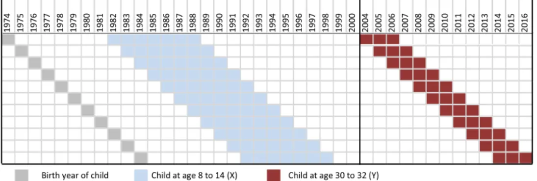
The study’s data are drawn from the ASSD (Zweim¨uller et al.,2009), a comprehensive database, covering all Austrians since the 1970s and offering detailed information about employment spells and wages collected by the Austrian Social Security Administration. We consider first born children born between 1974 and 1984 and link yearly personal and employment information on the parents to the children when they were between 8 and 14 years of age. This seven-year period will be referred to as ”period X”. Additionally, the panel captures relevant individual and labor market information about the children when they were 30 to 32 years old; this is denoted as ”period Y”.

We form yearly averages of the parents’ observational period X and the children’s final outcome period Y (see Figure 1). Furthermore, children whose father’s or mother’s main occupation during period X was a seasonal job or public service are dropped; these cases would confound our parental unemployment measure due to the excessively long periods of regular seasonal unemployment or unusually high employment protection. A small number of children with an obviously wrong (>365) sum of employment and unemployment days are also eliminated. Sim- ilarly, children who are simultaneously unemployed and retired are dropped from the sample.

The same logic is also applied to the parents. Missing information on parental education reduces the sample size further by a small degree. The excluded observations do not differ systematically from the rest of the sample, nor are there significant differences within the son/daughter subsamples.

Observing parents’ unemployment spells it is necessary to impose the requirement whereby the parents have to be formally employed during the childhood period of their offspring for a period of more than 365 days.

3.1 Descriptives

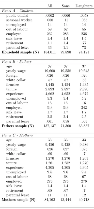
Table 1 reports the descriptives for the key variables. In panel A, the descriptives refer to all households exceeding 365 days of employment for both parents, while panels B and C are split into fathers and mothers, respectively. The overall sample comprises 154,011 individual children.

The share of females is 48.1%. The share of public officials is quite small, at around 0.6 %. There is also a small fraction (9%) of seasonal workers among children, of which sons account for the larger portion. The average parental age is 37 for fathers, and 33 for mothers. The mother’s yearly income is around 9,450 euros less than half that of the fathers, but these numbers include periods of non-work. The fathers tend to work in slightly larger firms than the mothers, while mothers tend to be employed in white collar jobs more frequently. As expected, parents do not differ according to the gender of their children.

(8)

The sample children are unemployed for 14 days and employed for 262 days per year on average, while they are out of the labor force for 59 days. Parental leave is granted for 36 days per year, almost entirely to females. Parents are on average unemployed 5.3 (fathers) or 9.5 (mothers) days per year. The fewer parental unemployment days compared to the children reflects the general increase in unemployment over time. Again, there are no systematic differences in parental labor market outcomes between sons and daughters.

The criteria for identifying mass layoffs adhere to the mandatory reporting guidelines of the Public Employment Service Austria (AMS). First, we exclude firms with fewer than 20 employees. For firms with 20 to 100 employees, a mass layoff is coded if at least five employees are dismissed; for firms of up to 600 employees, a mass layoff is coded if at least five percent of the workforce are dismissed; for firms with more than 600 employees, a mass layoff is coded if at least 30 workers are laid off. To measure the layoff size for each firm, we use a worker flow approach, which quantifies outgoing workers from one quartile to the next. We exclude firms that restructure, open new branches, or are involved in M&A, takeovers, or similar activities that cannot be classified as true mass layoffs. To do so, we identify joint movers, which are classified as a group of laid-off workers who make up at least 30 percent of all laid-off employees in their firm and move jointly to a new firm. Cases that formally exceed the thresholds of laid-off workers but include joint movers are not classified as mass layoffs. We provide more stringent measures of mass layoffs in section 8.

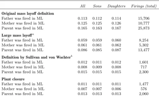
Table2summarizes the average likelihood of parents being dismissed in mass layoffs (ML). The numbers show that there was a 11.3% chance of a father being laid off in a firm that had a mass layoff in the period when the child was 8 to 14 years old. The risk for mothers was 12.5%, and the risk of either of the two being laid off was 16.5%. In a subsequent analysis, we use a simplified definition of mass layoffs formulated by Sullivan and von Wachter(2009), who define a mass layoff as a staff reduction by more than 30% of the firm’s peak employment during the last six years. In our data, plant closures are relatively rare. Only 1,601 men and 717 women lost their jobs due to a plant closure; this amounts to only 0.15% of parental pairs where at least one individual was laid off in a plant closure. Consequently, we cannot use plant closures as an exogenous shock on parental unemployment.

We measure the employment outcomes for the children when aged 30 to 32, for several reasons.

Most importantly, we want to use a longer observation period to avoid random effects and compare parents to children of similar ages, which is important for mitigating life-cycle biases between the parents and children. Children over 30 have likely finished their education (Black and Devereux, 2011). The study’s design is depicted in Figure 1. All variables are measured as yearly averages, unless stated differently in the specifications of the analysis and robustness checks.

(9)

Table 1: Descriptives - mean values All Sons Daughters Panel A - Children

public official .0062 .0066 .0058

seasonal worker .088 .11 .065

unemployed 14 14 14

out of labour 59 62 55

employed 262 286 236

sick leave 1.4 1.4 1.4

retirement 1.1 1.4 .77

parental leave 36 1.1 73

Household sample (N) 154,011 79,890 74,121 Panel B - Fathers

age 37 37 37

yearly wage 19,600 19,558 19,645

foreign .026 .026 .026

white collar .57 .57 .58

firmsize 1,445 1,454 1,435

tenure 2,893 2,897 2,890

experience 4,662 4,652 4,672

unemployed 5.3 5.4 5.2

retirement 2.5 2.4 2.5

parental leave .061 .058 .063

Fathers sample (N) 137,137 71,300 65,837 Panel C - Mothers

age 33 33 33

yearly wage 9,456 9,428 9,486

foreign .026 .027 .025

white collar .69 .69 .7

firmsize 1,270 1,276 1,263

tenure 1,261 1,252 1,270

experience 4,305 4,305 4,305

unemployed 9.5 9.6 9.4

retirement .68 .67 .7

parental leave 11 11 12

Mothers sample (N) 84,162 43,444 40,718

(10)

Table 2: Relative exposure - different layoff definitions

All Sons Daughters Firings (total) Original mass layoff definition

Father was fired in ML 0.113 0.112 0.114 15,706

Mother was fired in ML 0.125 0.125 0.126 10,777

Parent was fired in ML 0.165 0.163 0.167 25,873

Large mass layoff^a

Mother was fired in ML 0.061 0.061 0.062 5,302

Definition by Sullivan and von Wachter^b

Mother was fired in ML 0.008 0.009 0.008 717

Plant closure

Mother was fired in ML 0.007 0.007 0.006 576

Note: N= 154,011.^aa mass layoff is defined as large if the absolute number of laid off employees exceeds the median of the absolute number of laid off employees in the universe of all mass layoffs according to the original definition.^bdefinition of a mass layoff followingSullivan and von Wachter(2009)

.

4 Model and identification strategy

Our identification strategy aims to overcome the main causality issues discussed in sections 1 and 2. We compare the average parental unemployment days over seven years (X) with the unemployment days of the child in three periods (Y). We use an instrumental variables approach since possible confounding factors prohibit a causal interpretation of the effect of parents’ unemployment on children’s future unemployment. Specifically, we use the exogenous variation in being laid off in a mass layoff as an instrument for the unemployment days of the parent in period X. We argue that a mass layoff will exogenously increase the unemployment days of the parent, irrespective of family characteristics, genetics, or similar confounding factors simultaneously affecting parents and children. Most importantly, the shock has to be exogenous and there should be no selection into the treatment. It is conceivable that employees are being selected by employers into being laid off (first) during mass layoffs. We address this concern in section8 by considering only large layoffs, with a higher exogeneity of being laid off. The results support our assumption.

(11)

Figure 1: Periods of observation

1974 1975 1976 1977 1978 1979 1980 1981 1982 1983 1984 1985 1986 1987 1988 1989 1990 1991 1992 1993 1994 1995 1996 1997 1998 1999 2000 2004 2005 2006 2007 2008 2009 2010 2011 2012 2013 2014 2015 2016

Birth year of child Child at age 8 to 14 (X) Child at age 30 to 32 (Y)

Note: The years 2001 to 2003 are not in the figure, since they are not used in the analysis. The blue area covers information on the parents and the treatment, the red area includes employment outcomes of the children. Included controls are measured shortly or just before the beginning of the blue area.

The model’s objective function is

U Ei=α0+δU E_i^P +β⁰C+ζ⁰P+κcohort+πregion+i (1) where U E_i is the average number of unemployment days for child i in period Y and U E_i^P is the average number of unemployment days of the parent of childiin period X. Cis a vector of control variables for childicontaining sex and the number of siblings at the beginning of period X. The vector of control variables for the parent is P and includes sex, education, age at the beginning of period X, the number of unemployment days in the 10 years before period X, and foreignness.² κ_cohort captures cohort fixed effects, while π_region reflects regional fixed effects. _i is a random error. The concern that missing variables may influence parents’ and children’s unemployment experience makes an instrumental variables approach necessary.

The first stage is written as

U E^P_i =α0+γM Li+λ⁰C+ξ⁰P+τcohort+ρregion+νi (2) where U E_i^P is estimated as being laid off in a mass layoff, γM Li. γM Li = 1 if the parent has been laid off in a mass layoff, and 0 otherwise. All other parts of the function remain unaltered. A valid instrument requires that Cov(U E_i, M L_i|f(C,P)) = 0 andCov(M L_i, U E_i^P|f(C,P))6= 0.

We can easily show that the instrument has power (condition 2). The first condition posits that there should be no direct impact of the instrument, mass layoffs, on the unemployment experience of the children 20 years later over and above its impact via parental unemployment.

This requirement is easily fulfilled, unless serious long-term regional distortions occur after a massive layoff. We consider this case in our robustness analysis.

2We cannot completely observe all firm level covariates for the parents. Table A.2reports descriptives and the number of missing observations for a set of these covariates. We provide robustness checks including these (imputed) covariates at the end of this paper.

(12)

5 Results

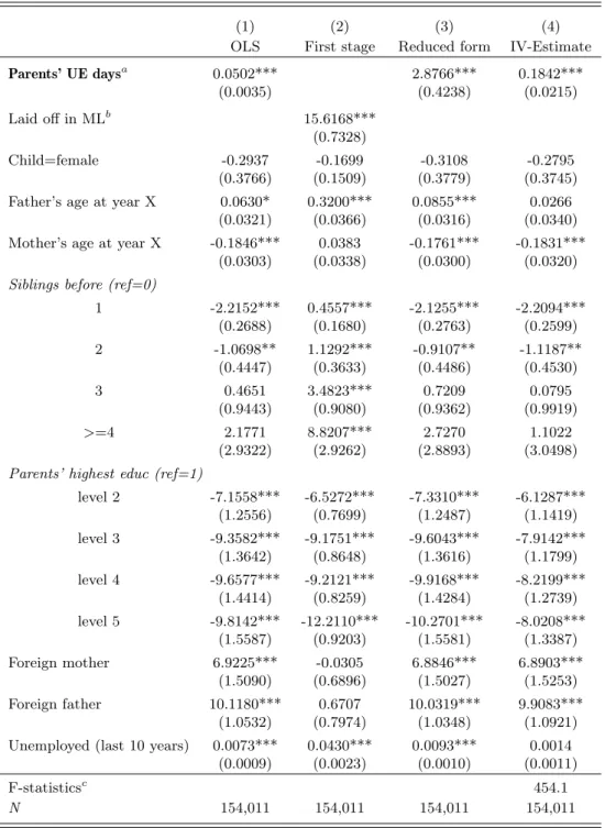
First, we discuss the effects of average parental unemployment on the unemployment experience of the children. The first column of Table 3 shows the OLS estimates of the effects of parental unemployment days during childhood on the number of unemployment days of the adult children.

The estimates suggest that an additional day of yearly average unemployment in period X increases the average number of unemployment days per year for adult children by 0.05 days.

However, this estimate cannot be interpreted causally. Column (2) shows a strong first-stage result for our instrumental variables model, showing that those laid off from their most recent firm have on average 16 more days of unemployment per year. Our instrumental variable is strong, as the F-statistics (Kleibergen and Paap, 2006) on the instrument are considerably above conventional levels. The reduced form (see Col. (3)) estimate confirms that a mass layoff of a parent positively correlates with the children’s later unemployment. Column (4) reports the estimate from the IV model with a magnitude of 0.18, which is significantly higher than the OLS estimate.

The control variables have the expected effects: A higher level of parental education lowers the intercept considerably compared to the baseline level, which is the lowest education. Mothers who are older in period Y seem to have a decreasing effect on the child’s future unemployment, while father’s age is irrelevant in the IV model. Parental foreignness appears to be a trigger for increased child unemployment. The number of siblings reduces the number of unemployment days for the children, but this effect vanishes with additional siblings. Increasing cohort fixed effects (not shown) again reflect the general trend of rising unemployment over time.

As a robustness check for our model in column (4), TableA.1in the appendix systematically adds covariates to a plain model. The results show that the estimated effect of parental unemployment on children’s unemployment is consistently stable.

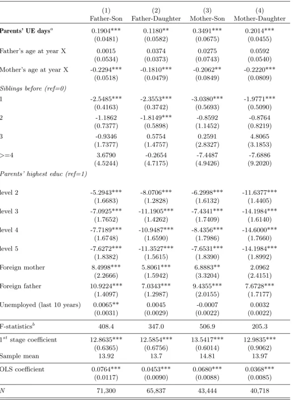
Table 4 lists the results for various parent-child combinations. The results suggest two main findings. First, sons seem to be more sensitive to increased parental unemployment during their childhood, and second, mothers seem to have a larger impact on the children in general. A test of the statistical significance of differences between the samples reveals that models (1) and (2) differ significantly, as do models (3) and (4). This confirms that sons are more sensitive to parental unemployment. A test of model (1) against (3) reveals that indifference cannot be rejected, while a test of (2) against (4) indicates that it can be rejected at the 5% level, suggesting that the finding that mothers exert a higher impact on children can be confirmed only for sons.

Why is the IV effect greater than the OLS outcomes? Prima facie, one would expect the opposite.

Unemployed fathers might have traits that are detrimental to the education of their children.

The downward bias of the OLS has two potential explanations. The first is measurement error.

We measure parental unemployment averaged over their children’s ages of 8 to 14 as a potential influence on the children’s development. While this is a natural age group to investigate, parents influence their children at all ages. The instrument takes care of this measurement error and thus magnifies the initial effect. The second reason could be our lack of information about preferences regarding family time and education. For instance, DelBoca et al. (2014) show a

(13)

positive correlation between parental dedication to their children and the children’s cognitive development and formal education. Parents who are thrown into a longer unemployment spell through a mass layoff may tend to be those with a lower preference to spend time with their children. The OLS estimate might be based on unemployment among parents with a high preference for family time and lower job commitment. If this is so, we would expect a downward bias in the OLS estimates.

Table 3: Causal impact of parents’ unemployment on children’s unemployment

(1) (2) (3) (4)

OLS First stage Reduced form IV-Estimate

Parents’ UE days^a 0.0502*** 2.8766*** 0.1842***

(0.0035) (0.4238) (0.0215)

Laid off in ML^b 15.6168***

(0.7328)

Child=female -0.2937 -0.1699 -0.3108 -0.2795

(0.3766) (0.1509) (0.3779) (0.3745) Father’s age at year X 0.0630* 0.3200*** 0.0855*** 0.0266

(0.0321) (0.0366) (0.0316) (0.0340) Mother’s age at year X -0.1846*** 0.0383 -0.1761*** -0.1831***

(0.0303) (0.0338) (0.0300) (0.0320) Siblings before (ref=0)

1 -2.2152*** 0.4557*** -2.1255*** -2.2094***

(0.2688) (0.1680) (0.2763) (0.2599)

2 -1.0698** 1.1292*** -0.9107** -1.1187**

(0.4447) (0.3633) (0.4486) (0.4530)

3 0.4651 3.4823*** 0.7209 0.0795

(0.9443) (0.9080) (0.9362) (0.9919)

>=4 2.1771 8.8207*** 2.7270 1.1022

(2.9322) (2.9262) (2.8893) (3.0498) Parents’ highest educ (ref=1)

level 2 -7.1558*** -6.5272*** -7.3310*** -6.1287***

(1.2556) (0.7699) (1.2487) (1.1419) level 3 -9.3582*** -9.1751*** -9.6043*** -7.9142***

(1.3642) (0.8648) (1.3616) (1.1799) level 4 -9.6577*** -9.2121*** -9.9168*** -8.2199***

(1.4414) (0.8259) (1.4284) (1.2739) level 5 -9.8142*** -12.2110*** -10.2701*** -8.0208***

(1.5587) (0.9203) (1.5581) (1.3387)

Foreign mother 6.9225*** -0.0305 6.8846*** 6.8903***

(1.5090) (0.6896) (1.5027) (1.5253)

Foreign father 10.1180*** 0.6707 10.0319*** 9.9083***

(1.0532) (0.7974) (1.0348) (1.0921) Unemployed (last 10 years) 0.0073*** 0.0430*** 0.0093*** 0.0014

(0.0009) (0.0023) (0.0010) (0.0011)

F-statistics^c 454.1

N 154,011 154,011 154,011 154,011

Notes: For columns (1), (3), and (4) the dependent variable is the average yearly unemployment days of the child during the age of 30 to 32.

Column (2) represents the first stage coefficient with average yearly unemployment days of the parents as dependent variable. All estimations include cohort and regional fixed effects. Regional-level clustered standard errors in parentheses,^∗p <0.10,^∗∗p <0.05,^∗∗∗p <0.01.^aParents’

UE days represents the average number of unemployment days per year for both parents. ^bLaid off in ML is a dummy equal to 1 if at least one of the parents was laid off in a mass layoff, 0 otherwise.^bKleibergen and Paap(2006) statistics on the instrument in the first stage.

(14)

Table 4: IV results for parent-child combinations

(1) (2) (3) (4)

Father-Son Father-Daughter Mother-Son Mother-Daughter Parents’ UE days^a 0.1904*** 0.1180** 0.3491*** 0.2014***

(0.0481) (0.0582) (0.0675) (0.0455)

Father’s age at year X 0.0015 0.0374 0.0275 0.0592

(0.0534) (0.0373) (0.0743) (0.0540)

Mother’s age at year X -0.2294*** -0.1810*** -0.2062** -0.2220***

(0.0518) (0.0479) (0.0849) (0.0809)

Siblings before (ref=0)

1 -2.5485*** -2.3553*** -3.0380*** -1.9771***

(0.4163) (0.3742) (0.5693) (0.5090)

2 -1.1862 -1.8149*** -0.8592 -0.8764

(0.7377) (0.5898) (1.1452) (0.8219)

3 -0.9346 0.5754 0.2591 4.8065

(1.7377) (1.4757) (2.8327) (3.1853)

>=4 3.6790 -0.2654 -7.4487 -7.6886

(4.5244) (4.7175) (4.9426) (9.2020)

Parents’ highest educ (ref=1)

level 2 -5.2943*** -8.0706*** -6.2998*** -11.6377***

(1.6683) (1.2828) (1.6132) (1.4405)

level 3 -7.0925*** -11.1905*** -7.4341*** -14.1984***

(1.7652) (1.4262) (1.7409) (1.6140)

level 4 -7.7189*** -10.9487*** -8.4356*** -14.6000***

(1.6748) (1.6590) (1.7986) (1.7660)

level 5 -7.6272*** -11.3527*** -7.6531*** -14.1984***

(1.8382) (1.5615) (1.8390) (1.8992)

Foreign mother 8.4998*** 5.8061*** 6.8883** 2.0962

(2.2666) (1.5942) (3.3204) (2.4151)

Foreign father 10.9224*** 7.0343*** 9.4355*** 7.6728***

(1.4097) (1.2987) (2.0155) (1.7177)

Unemployed (last 10 years) 0.0065** 0.0045 -0.0007 0.0032

(0.0031) (0.0029) (0.0022) (0.0022)

F-statistics^b 408.4 347.0 506.9 205.3

1^ststage coefficient 12.8635*** 12.5854*** 13.5417*** 12.9835***

(0.6365) (0.6756) (0.6014) (0.9062)

Sample mean 13.92 13.7 14.81 13.97

OLS coefficient 0.0764*** 0.0453*** 0.0680*** 0.0368***

(0.0117) (0.0090) (0.0088) (0.0085)

N 71,300 65,837 43,444 40,718

Notes: IV results. The dependent variable is the average yearly unemployment days of the child during the age of 30 to 32. All estimations include cohort and regional fixed effects. Regional-level clustered standard errors in parentheses,^∗p <0.10,^∗∗p <0.05,^∗∗∗p <0.01.

aParents’ UE days represents the average number of unemployment days per year for fathers in models (1) and (2), and mothers in models (3) and (4).

bKleibergen and Paap(2006) statistics on the instrument in the first stage.

(15)

6 Effect heterogeneity

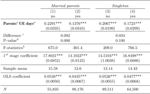
Our discussion so far has been limited to overall effects. In this section we deepen our under- standing of the transmission process for the sample’s subgroups. Table5 splits the sample into married vs. unmarried parents at the beginning of period X. Unmarried parents can be either never married or divorced. The table also reports whether the effects differ statistically from one another. Unmarried parents have a significantly stronger transmission of unemployment than married parents which may be due to a stronger (and more unique) role model effect. Another reason might be the fact that loss of income sources is more severe for a single parent.

Columns (3) and (4) report the effects for singleton children and children with siblings. The intergenerational transmission of unemployment is somewhat stronger for children who have siblings at the beginning of period X.

Table 5: Effect heterogeneity - Family background

Married parents Singleton

(1) (2) (3) (4)

no yes no yes

Parents’ UE days^a 0.2291*** 0.1376*** 0.2067*** 0.1725***

(0.0335) (0.0310) (0.0199) (0.0299)

Difference^c 0.092 0.034

P-value^d 0.000 0.100

F-statistics^b 675.0 301.4 209.0 766.5

(0.6852) (0.8123) (1.0038) (0.6086)

Sample mean 15.58 12.6 13.14 14.43

OLS coefficient 0.0538*** 0.0435*** 0.0526*** 0.0477***

(0.0050) (0.0067) (0.0055) (0.0068)

N 55,835 98,176 89,511 64,500

Notes: IV results. The dependent variable is the average yearly unemployment days of the child during the age of 30 to 32. Models (1) and (2) are a split by the marital status at the beginning of period X. Models (3) and (4) are split by whether the child is a singleton child up to the end of period X. All estimations include control variables from the main specification (siblings excluded as control in column (3) and (4)) as in Table3, as well as cohort and regional fixed effects. Regional-level clustered standard errors in parentheses,^∗p <0.10,^∗∗p <0.05,^∗∗∗p <0.01.

aParents’ UE days represents the average number of unemployment days per year for both parents.

cBootstrap and permutation test for difference in coefficients between groups (Permutations=100).

dReported p-value for difference in coefficients.

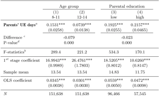
Next, we explore whether child age (at the time of parental unemployment) or parental education is instrumental for the intergenerational correlation. Table 6 reports the results of splitting the age range for children in two groups: ages 8 to 11 in column (1) and ages 12 to 14 in column (2). The intergenerational correlation is significantly greater if parental unemployment happens when the child is between 8 and 11 years old. This age range coincides with the decision to send the child to high-school or not. ³

3Austria has a school system with an early tracking schedule whereby students can proceed to an academic track or more practical studies when they turn 10.

(16)

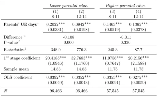
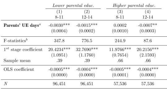
Columns (3) and (4) reveal that intergenerational transmission is stronger for the more highly educated parents. Table 7 digs deeper in this issue by interacting these two dimensions. We show the effects for both age groups separately for high and low parental education. An age difference is observed only for low-education parents (Cols. (1) and (2)). A large intergenerational transmission of unemployment occurs for low-education parents when the child is between 8 and 11. The effect is only half as strong if parental unemployment occurs when the child is between 12 and 14. This demonstrates the great importance of school selection.

Table 6: Effect heterogeneity - Age and parental education

Age group Parental education

(1) (2) (3) (4)

8-11 12-14 low high

Parents’ UE days^a 0.1531*** 0.0739*** 0.1925*** 0.2157***

(0.0258) (0.0138) (0.0255) (0.0465)

Difference^c -0.079 -0.023

P-value^d 0.000 0.000

F-statistics^b 289.4 221.2 534.3 170.1

(0.9989) (1.7803) (0.8012) (0.8147)

Sample mean 13.54 13.54 14.83 11.75

OLS coefficient 0.0345*** 0.0301*** 0.0559*** 0.0472***

(0.0038) (0.0030) (0.0050) (0.0098)

N 151,638 151,638 96,466 57,545

Notes: IV results. The dependent variable is the average yearly unemployment days of the child during the age of 30 to 32. Models (1) and (2) are separate regressions defined for age groups of 8-11 and 12-14 years. Models (3) and (4) are split by whether the highest achieved education of the parents is above an equivalent of a graduation diploma (Matura). All estimations include control variables from the main specification (parents’ education excluded as control in column (3) and (4)) as in Table3, as well as cohort and regional fixed effects. Regional-level clustered standard errors in parentheses,^∗p <0.10,^∗∗p <0.05,^∗∗∗p <0.01.

cBootstrap and permutation test for difference in coefficients between groups (Permutations=100).

dReported p-value for difference in coefficients.

7 Transmission channels

Why are the intergenerational transmissions so large? As mentioned, education is an obvious factor. Parental unemployment might hinder the children’s educational choices or potential (Coelli, 2011; Jones, 1988; Rege et al., 2011). We explore this possibility in Tables 8 and 9. A second mechanism might involve family networks and structure. Unemployment may reduce parental networks, which may reduce the children’s job-finding capacity (Plug et al., 2018). Moreover, parental unemployment might increase tension within the family, leading to a higher chance of divorce, which may influence the adult child’s labor market outcomes (De-Goede et al., 2000; Str¨om, 2003). This possibility is explored in Table 10. Finally, the effects of income deprivation due to parental unemployment are investigated in Table11. Other,

(17)

Table 7: Age groups by parental education

Lower parental educ. Higher parental educ.

(1) (2) (3) (4)

8-11 12-14 8-11 12-14

Parents’ UE days^a 0.2022*** 0.0942*** 0.1463*** 0.1365***

(0.0331) (0.0198) (0.0519) (0.0378)

Difference^c -0.108 -0.011

P-value^d 0.000 0.330

F-statistics^b 348.0 776.3 245.3 87.7

1^st stage coefficient 20.4185*** 32.7683*** 11.9756*** 20.2156***

(1.0946) (1.1760) (0.7647) (2.1588)

Sample mean 14.83 14.83 11.75 11.75

OLS coefficient 0.0392*** 0.0352*** 0.0355*** 0.0275***

(0.0040) (0.0043) (0.0091) (0.0059)

N 96,466 96,466 57,545 57,545

Notes: IV results. The dependent variable is the average yearly unemployment days of the child during the age of 30 to 32. Samples are split by the age of the observed child during period X, as well as the highest achieved education of the parents is above or equal high-school graduation (Matura). All estimations include control variables from the main specification (except parents’ education) as in Table3, as well as cohort and regional fixed effects. Regional-level clustered standard errors in parentheses,^∗p <0.10,^∗∗p <0.05,^∗∗∗p <0.01.

potential transmission channels are related to changes in the work ethics of the unemployed parents; however, such channels cannot be tested using administrative data.

Table 8 shows the instrumental variable estimates for the effect of parental unemployment on the education of the offspring: years of education, education above the median, and tertiary education ⁴ are used as dependent variables. While we find no significant negative effects on tertiary education, 100 additional days of parental unemployment reduce education by 0.72 years and reduce the probability of being above the median by 0.18 percentage points. These results stress the importance of education.

Table9 explores the role of education further by considering parental background — which has been found to be a very strong predictor of children’s education (Black et al.,2005) — and child age as conditioning factors. Table 9 is similar to Table 7, but, instead of looking at children’s unemployment, Table 9 considers the probability that children’s education is greater than the median. As in Table 7, we see larger effects for parents with low education. Among this group, the greatest effect is for children at the critical age of 10, when key educational decisions have to be made. However, the results for more highly educated parents are substantially different.

We observe no significant effect of parental unemployment on the probability of children aged 8 to 11 completing high-school. The effect is significant but small for children aged 12 to 14.

4As several values are missing, we imputed the education variable using the random forest method. The results are robust to the use of generic education only, which involves a smaller sample size.

(18)

Table 8: Educational choice of children

(1) (2) (3)

years better tertiary Parents’ UE days^a -0.0072*** -0.0018*** -0.0005 (0.0019) (0.0004) (0.0003)

F-statistics^b 453.6 453.6 453.6

1^st stage coefficient 15.6163*** 15.6163*** 15.6163***

(0.7332) (0.7332) (0.7332)

Sample mean 13.28 .49 .25

OLS coefficient -0.0024*** -0.0004*** -0.0002***

(0.0002) (0.0000) (0.0000)

N 153,987 153,987 153,987

Notes: IV results. The dependent variable is years of education of the child in model (1), a binary variable equal to 1 if the child’s highest education is above middle school in model (2), a binary equal to 1 if the child has a university degree in model (3). All estimations include control variables from the main specification as in Table3, as well as cohort and regional fixed effects. Regional-level clustered standard errors in parentheses,^∗p <0.10,^∗∗p <0.05,^∗∗∗p <0.01.

Table 9: Educational choice of children by age group and parental education – above or below the median Lower parental educ. Higher parental educ.

(1) (2) (3) (4)

8-11 12-14 8-11 12-14

Parents’ UE days^a -0.0030*** -0.0015*** 0.0002 -0.0007**

(0.0004) (0.0002) (0.0010) (0.0003)

F-statistics^b 347.8 776.5 244.9 87.6

(1.0951) (1.1760) (0.7654) (2.1593)

Sample mean .39 .39 .66 .66

OLS coefficient -0.0005*** -0.0004*** -0.0005*** -0.0004***

(0.0000) (0.0000) (0.0001) (0.0000)

N 96,451 96,451 57,536 57,536

Notes: IV results. The dependent variable is 1 if the if the observed child’s educational attainment is above or equal high-school graduation (Matura), 0 else. Samples are split by the age of the observed child during period X, as well as the highest achieved education of the parents is above or equal high-school graduation (Matura). All estimations include control variables from the main specification (except parents’

education) as in Table3, as well as cohort and regional fixed effects. Regional-level clustered standard errors in parentheses,^∗p <0.10,^∗∗p <

0.05,^∗∗∗p <0.01.

While the results for low-education parents indicate an educational transmission, the small results for high-education parents show that educational transmission cannot be the only expla- nation for the intergenerational transmission of unemployment.

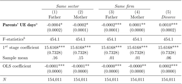
The second hypothesis concerns parental networks and family structure. Table 10 shows the results of IV regressions testing whether, at the beginning of period Y the child works in the same sector or in the same firm as one of the parents, which might be due to a parental job

(19)

Table 10: Plausible transmission channels: Family network and disruption

Same sector Same firm

(1) (2) (3) (4) (5)

Father Mother Father Mother Divorce

Parents’ UE days^a -0.0004* -0.0002* -0.0002*** 0.0001** 0.0010***

(0.0002) (0.0001) (0.0001) (0.0000) (0.0002)

F-statistics^b 454.1 454.1 454.1 454.1 454.1

1^st stage coefficient 15.6168*** 15.6168*** 15.6168*** 15.6168*** 15.6168***

(0.7328) (0.7328) (0.7328) (0.7328) (0.7328)

Sample mean .16 .15 .01 .01 .06

OLS coefficient -0.0001*** -0.0001** -0.0000*** -0.0000** 0.0002***

(0.0000) (0.0000) (0.0000) (0.0000) (0.0000)

N 154,011 154,011 154,011 154,011 154,011

Notes: IV results. The dependent variable is a binary equal to 1 if the child works in the same sector (NACE08) as the father or mother, for models (1) and (2), respectively. The dependent variable is a binary equal to 1 if the child works in the same firm as the father or mother, for models (3) and (4), respectively. The dependent variable is a binary equal to 1 if the parents divorced between the periods X and Y in model (5), 0 otherwise. All estimations include control variables from the main specification as in Table3, as well as cohort and regional fixed effects. Regional-level clustered standard errors in parentheses,^∗p <0.10,^∗∗p <0.05,^∗∗∗p <0.01.

network, and whether the parents get divorced. The results show that both job networks and family disruptions matter: 100 additional days of the father’s (mother’s) unemployment reduce the probability of the child being in the same sector by 0.04 (0.02) percentage points. The negative effects of being in the same firm – an even stronger indication of network effects – are around half of that. These are relatively large effects. We also see that the divorce probability is increased.

In addition to less access to education and reduced parental network effectiveness, income deprivation because of unemployment is another potentially important channel for intergenerational unemployment transmission. Lower family income is found to have negative effects on child achievement and labor market outcomes (Dahl and Lochner, 2012). Unfortunately, our data does not provide detailed information on working hours and hourly wages to proxy potential household income. Moreover, information on income of parents in our data is polluted by bonus payments, severance payments, as well as unemployment spells without detailed information on unemployment benefits. Consequently, we construct a variable for measuring potential household income, which measures the potential wage a household can expect given all observed household characteristics.⁵

Table 11 presents the estimation results for our main model for four quartiles of the potential household income. We estimate a positive and significant effect of parental unemployment days on children’s unemployment days for all quartiles of the potential income distribution. If income

5Potential income is calculated on a yearly basis as [observed actual income/days employed]*calendar days. To avoid unreasonable results from possible retroactive or bonus payments on a single day we restrict the potential income computation to workers with at least 31 days of employment in a given year. We impute missing values with means by year, sex, age, education, and foreignness. If neither actual income, nor employment days are observed, potential income is coded as missing. Figure2in the appendix provides kernel density estimations for actual and potential income in our sample.

(20)

loss were the primary source of the intergenerational transmission of unemployment, families in the top quartile would show the smallest effect, if any. Top-earning families are expected to have high financial reserves and could expect to find a job relatively quickly after a mass layoff.

Consequently, we conclude that income loss cannot be the main driving force for the observed intergenerational correlation.

Table 11: Average potential income quartiles of the households

(1) (2) (3) (4)

Q1 Q2 Q3 Q4

Parents’ UE days^a 0.1295*** 0.2514*** 0.1361** 0.2096***

(0.0298) (0.0404) (0.0517) (0.0602)

F-statistics^b 510.4 509.1 235.9 127.1

1^st stage coefficient 19.9112*** 17.6763*** 13.7042*** 9.8711***

(0.8813) (0.7834) (0.8923) (0.8755)

Sample mean 15.96 14.18 12.49 12.11

Upper threshold (income) 30,773.15 36,461.69 42,589.8 98,423.55 OLS coefficient 0.0492*** 0.0318*** 0.0658*** 0.0444***

(0.0060) (0.0053) (0.0107) (0.0120)

N 38,495 38,495 38,494 38,494

Notes: IV results. The dependent variable is the average yearly unemployment days of the child during the age of 30 to 32. Columns (1) to (4) present results for separate samples in each potential income quartile 1 to 4, respectively. The upper threshold marks the maximum value of potential income for each quartile. All estimations include control variables from the main specification as in Table3, as well as cohort and regional fixed effects. Regional-level clustered standard errors in parentheses,^∗p <0.10,^∗∗p <0.05,^∗∗∗p <0.01.

8 Robustness checks

This section explores several problems with our instrumental variables strategy: i) mass layoffs could be selective and hit a very specific group of workers, and ii) the exclusion restriction could be violated if a mass layoff had an independent effect on children 20 years later. Such an effect could happen if a (large) mass layoff caused serious long-term distortions on a local or regional labor market (Foote et al.,2019;Gathmann et al.,2018). In such a situation, the labor market would continue to be weaker due to this mass layoff.

We try to capture the first effect by changing the study’s mass layoff definition. We first define a situation as a mass layoff only if it is above the median size (in terms of the absolute number of dismissed employees) of all mass layoffs. Second, and more conservatively, we use a definition drawn from Sullivan and von Wachter(2009), whereby a layoff affecting more than 30% of the firms’ peak employment over the last six years is defined as a mass layoff.⁶

6We deviate from the original definition by also including firm histories shorter than six years if they are not available for the full length. Furthermore, we set the minimum firm size to 20 instead of 50 employees and place no restrictions on employee tenure.