On the Price of Anarchy for flows over time JOSÉ CORREA and ANDRÉS CRISTI,

On the Price of Anarchy for flows over time

JOSÉ CORREA and ANDRÉS CRISTI,Universidad de Chile, Chile

TIM OOSTERWIJK,Maastricht University, Netherlands

Dynamic network flows, or network flows over time, constitute an important model for real-world situations where steady states are unusual, such as urban traffic and the Internet. These applications immediately raise the issue of analyzing dynamic network flows from a game-theoretic perspective. In this paper we study dynamic equilibria in the deterministic fluid queuing model in single-source single-sink networks, arguably the most basic model for flows over time. In the last decade we have witnessed significant developments in the theoretical understanding of the model. However, several fundamental questions remain open. One of the most prominent ones concerns the Price of Anarchy, measured as the worst case ratio between the minimum time required to route a given amount of flow from the source to the sink, and the time a dynamic equilibrium takes to perform the same task. Our main result states that if we could reduce the inflow of the network in a dynamic equilibrium, then the Price of Anarchy is exactly e/(e−1) ≈1.582. This significantly extends a result by Bhaskar, Fleischer, and Anshelevich (SODA 2011). Furthermore, our methods allow to determine that the Price of Anarchy in parallel-link networks is exactly 4/3. Finally, we argue that if a certain very natural monotonicity conjecture holds, the Price of Anarchy in the general case is exactly e/(e−1).

CCS Concepts: •Theory of computation→Algorithmic game theory;Quality of equilibria;Network games;Routing and network design problems; •Mathematics of computing→Network flows; •Networks

→Network dynamics.

Additional Key Words and Phrases: flows over time, price of anarchy, dynamic equilibrium ACM Reference Format:

José Correa, Andrés Cristi, and Tim Oosterwijk. 2019. On the Price of Anarchy for flows over time. InACM EC

’19: ACM Conference on Economics and Computation (EC ’19), June 24–28, 2019, Phoenix, AZ, USA.ACM, New York, NY, USA, 19 pages. https://doi.org/10.1145/3328526.3329593

1 INTRODUCTION

In the study of traffic in networks it is often crucial to take the underlying dynamical nature of the problem into account. In some contexts steady states seem sufficient to deal with the most important situations and therefore static models are enough. However, the situation is dramatically different when dealing with networks where a steady state is rarely observed such as urban traffic or Internet routing. In order to describe the temporal evolution of such systems one has to consider the propagation of flow across the network by tracking the position of each particle along time.

Probably the most basic model for network flows over time is the so-calledfluid queuing model. Here, we are given a directed graphG =(V,E)and each edgee ∈Eis characterized by a non- negative delayτe and a capacity per time unitνe. A continuous stream of particles is injected at a sources ∈V, at constant rateu0, and travels towards a sinkt∈V. Flow propagates according to the edge dynamics in which particles arriving to an edgeejoin a queue with (deterministic) service rateνe and, after leaving the queue, move along the edge to reach its head afterτe time units. The

Permission to make digital or hard copies of all or part of this work for personal or classroom use is granted without fee provided that copies are not made or distributed for profit or commercial advantage and that copies bear this notice and the full citation on the first page. Copyrights for components of this work owned by others than ACM must be honored.

Abstracting with credit is permitted. To copy otherwise, or republish, to post on servers or to redistribute to lists, requires prior specific permission and /or a fee. Request permissions from permissions@acm.org.

EC ’19, June 24–28, 2019, Phoenix, AZ, USA

© 2019 Association for Computing Machinery.

ACM ISBN 978-1-4503-6792-9/19/06. . . $15.00 https://doi.org/10.1145/3328526.3329593

discrete version of the problem was initially studied from an optimization perspective. Indeed, Ford and Fulkerson [10, 11] considered a fluid queuing model and designed an algorithm, based on time expanded networks, to compute a flow over time carrying the maximum possible flow from the sourcesto the sinktwithin a given timespan. Shortly after, Gale [12] showed the existence of a flow pattern that achieves this optimum simultaneously for all time horizons. These results were extended to continuous time by Anderson and Philpott [1] and Fleischer and Tardos [9]. We refer to the survey by Skutella [28] for a detailed exposition of these developments.

When network flows suffer from a lack of coordination among the participating agents, it is natural to consider them from a game-theoretic perspective. In this setting, each infinitesimal inflow particle is interpreted as a player that seeks to complete its journey in the least possible time, so that equilibrium occurs when each particle travels along a shortests,t-path. The travel time for a particle entering the network at any given time must take into account the queuing delays induced by other particles on the edges along its path. This requires particles to anticipate the queue lengths by the time when an edge will be reached.

Thisdynamic equilibriummodel was initially considered, in a very simple network, by Vickrey [30], and shortly after in the transportation science community [31]. Since then it has attracted much attention as a showcase model to understand the surprising behavior of dynamic routing games [23, 24]. In the last decade there have been significant efforts in understanding the structure and computational properties of dynamic equilibria in the fluid queuing model [3–8, 14, 16, 17, 19, 22, 25–

27]. Meunier and Wagner [22] proved, using functional analysis tools, that such dynamic equilibria exist. Unfortunately, this result (and many similar ones) is purely existential and does not shed light on the structure of such equilibria. Later, Koch and Skutella [19] gave an elegant characterization of the derivatives (w.r.t. time) of a dynamic equilibrium and thus proposed an algorithm to construct a dynamic equilibrium by concatenating static flows. Using this characterization, Cominetti, Correa and Larré [7] gave a constructive proof of existence of equilibria and proved they are essentially unique. Despite these efforts, many fundamental questions remain open, and several apparently obvious properties turn out to be notoriously hard to prove. For instance, it is still unknown whether a dynamic equilibrium can be computed in polynomial time, and furthermore, we do not even know whether the evolution of the equilibrium has finitely many pieces. Indeed, until recently, it was not even known whether the size of the queues remains bounded throughout the evolution of the dynamic equilibrium. Along these lines, Cao et al. [5] established this property (on a slightly different atomic model that does not influence the result) for series-parallel networks, while Correa et al [8] established the result for general networks by proving that a steady state is always achieved in finite time (naturally, as long asu⁰is at most the capacity of the minimum cut). Quite surprisingly however, the latter results apply only for constant inflow rateu0; if the inflow varies over time, say it isu0in all intervals of the form[2i,2i+1)andu0/2 in all intervals of the form[2i−1,2i)for i ∈N, then the boundedness of the queues is still open.

Another seemingly innocent question regarding the dynamic equilibrium is what we call the monotonicity conjecture(cf. Conjecture 3). This states that given an instance of the problem, the time it takes for an amount of flow to reach the sinktis a decreasing function of the inflow rate u0. In other words, if we consider two identical instances, one with constant inflow rateu0and the other with constant inflow rateu⁰−ε, then the time it takes forMflow units to arrive att in the latter instance is at least that in the former. As we show in this paper, this conjecture is intimately connected to one of the most prominent open problems in the area, namely, the quality of the equilibrium (measured as the time required to send a given amount of flow fromstot) when compared to the optimal solution. Our main result, which can be seen as an improvement upon a result of Bhaskar, Fleischer and Anshelevich [3, 4], establishes that if the monotonicity conjecture

holds for the dynamic equilibrium, then the Price of Anarchy, defined as the worst case ratio of the quality of an equilibrium to that of an optimal solution, is exactly e/(e−1).

1.1 The Price of Anarchy

The usual way of quantifying the inefficiency of selfish behavior is the Price of Anarchy (PoA). It is defined as the worst possible ratio between the quality of an optimal solution and the quality of an equilibrium [20]. In the context of fluid queuing networks there are two natural and related goals which induce two natural possible definitions for the PoA. On the one hand, we have thethroughput objective, under which we are given a time window and are asked to maximize the amount of flow that can reach the sinkt within that time. On the other hand, we have themakespanobjective, under which we are given an amount of flowM, that needs to be routed totin the shortest possible time.

The existence of anearliest arrival flow, established by Gale [12], implies that from an optimization viewpoint, both goals are equivalent. Nevertheless, they induce different notions for the PoA. In the former case the throughput-PoA is, as usual, defined as the supremum over all singles,t-graphs, all possible inflows, all possible capacities, all possible transit times, and all possible time windows, of the ratio between the amount of flow the optimal solution can send and the amount of flow a dynamic equilibrium sends. In the latter case the makespan-PoA is defined as the supremum over all singles,t-graphs, all possible inflows, all possible capacities, all possible transit times, and all possible amounts of flowM, of the ratio between the time the optimal solution takes to routeM units of flow towardstand the time it takes in a dynamic equilibrium.

The first to study the PoA in this context were Koch and Skutella [18, 19] who proved that the throughput-PoA is unbounded. They also show that if the delays of all edges are zero, then the dynamic equilibria are optimal, implying that both the throughput-PoA and the makespan-PoA are 1. Interestingly, it has long been conjectured that the makespan-PoA is bounded by a small constant [29]. The study of this makespan-PoA measure is the main focus of this paper, which from now on we just call PoA for short.

Beyond the zero delay case, Bhaskar, Fleischer and Anshelevich [3, 4] studied this question from a mechanism design perspective and found that there is a way of reducing the capacities in the network so that the makespan of an equilibrium under the reduced capacities is within a factor e/(e−1)of the optimal solution with the original capacities. Naturally, as the following example demonstrates, this capacity reduction can improve the behavior of a dynamic equilibrium by blocking particles from taking bad routes.

However, the result still requires a subtle analysis since reducing the capacities too much may also block good routes significantly, increasing the makespan of a dynamic equilibrium. More precisely, Bhaskar et al. consider reducing the capacity of every edgeeto be exactly the amount of flow rate the optimal solution propagates throughe. Our main result is to establish that the same bound still holds by doing this only for the inflow, i.e., leaving all capacities unchanged but only reducing the inflow.

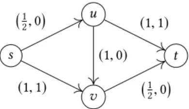
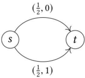
Example1. Consider the network in Fig. 1, where an edgeeis labelled(νe,τe), and let the total flowMto be sent through the network be 2 and letu⁰ =1. We claim that the optimal flow will send¹

2 units of flow both along the path(s,u,t)and along the path(s,v,t)until time 2. Therefore, the makespan of the optimal flow is 3. On the other hand, the equilibrium will first send 1 unit of flow along the path(s,u,v,t)from time 0 until time 1. Then, from time 1 to 2, it will send¹

2 units of flow both along the path(s,u,v,t)and along the path(s,v,t). Since a particle originating atsat time 2 will encounter a queue time of 1 on edges(s,u)and(v,t), the makespan of the equilibrium

s

u

v

t

1 2,0

(1,1)

(1,0) (1,1)

1 2,0

Fig. 1. An illustration of the network of Example 1.

is 4, and hence, the PoA of this instance is ⁴

3. Note that if we setνuv =0 (as in [4]), the equilibrium in the modified network will do exactly the same as the optimal flow, and the new PoA is 1.

Finally, Cominetti, Correa and Olver [8] prove the existence of a steady state and furthermore establish that the derivative of this steady state flow is the solution of the static minimum cost problem in which the cost of edgeeis given byτeand the capacity byνe. This result readily implies that the Price of Anarchy converges to 1 as the amount of flow to be routed grows to infinity.

1.2 Our results

As mentioned above, our main result is to improve upon the result of Bhaskar, Fleischer and Anshelevich [3, 4] and show that the PoA is upper bounded by e/(e−1)under the milder assumption that the inflow rate of the equilibrium is equal to the (initial) inflow rate of the optimum flow. This is a theoretical improvement since it potentially makes further progress (e.g. on multi-commodity settings) on this problem easier. Moreover, it can be of practical relevance because inflow-limiting mechanisms are easier to implement and currently used in many places, such as metered ramps on highways.

For a networkGand a total amount of flowM, denote byTOPT the time the optimal flow takes to route theMunits fromstot. The simplest algorithm to compute this quantity is that of Ford and Fulkerson [11] which we describe in Section 2.1. The basic idea is to guessT =TOPT and then find a static flowf maximizing|f|T −Í

e∈Eτefe, where |f|denotes the size of the flow and is constrained to be at mostu0. We denote the inflow rate of the optimal flow byuOPT =|f|. As in the dynamic equilibrium particles are selfish, its inflow rateuEQalways equalsu0.

Similarly, lettingTEQ be the time it takes for the equilibrium to route theMunits of flow,¹our main result, which we prove in Section 3, can be stated in the following terms.

Theorem 2. IfuEQ =uOPT, thenTEQ ≤_e−1^e ·TOPT and this is tight.

Note thatuEQ =u⁰ ≥uOPT, therefore the missing case left by Theorem 2 is whenuEQ >uOPT. Intuitively, this case should be easier. Indeed, for the theorem to hold in general it is enough to prove the monotonicity conjecture, which basically states that by decreasing the inflow, the makespan TEQincreases. To formalize this conjecture, denote the makespan of the equilibrium with inflow rateu_ibyT_EQⁱ .

Conjecture 3(Monotonicity conjecture). Consider a networkGand two fixed inflow ratesu1<u2

with their corresponding dynamic equilibria inG. ThenT_EQ¹ ≥T_EQ² .

For the special and simpler case of parallel-link networks, it turns out that the monotonicity conjecture holds (cf. Lemma 16), immediately implying, by Theorem 2, that the PoA is bounded for these networks. Furthermore, for parallel-link networks we are able to obtain an improved bound

1

In Section 2.2 we denote byθˆ=M/u0the time this last particle enterssand byℓt(θ)ˆ the time at which it reachest. Since the dynamic equilibrium satisfies FIFO, it is clear thatℓ_t(θˆ)=T_EQ.

by refining the analysis. In fact, the argument can be extended to parallel-path networks. Indeed, we prove the following result.

Theorem 4. In parallel-link networks,TEQ ≤ ⁴₃·TOPT and this is tight.

The proofs proceed in three basic steps. First, we establish that the difference between the makespansT_EQ−T_OPT is upper bounded by the overall sum of the queues at equilibrium divided by its inflow. This follows from the linear program that computes the optimal solution, combined with the equilibrium conditions stating that particles are routed through (currently) shortest paths.

Second, we establish a formula for computing this sum of the queues at equilibrium in terms of the derivatives of the dynamic equilibrium (thin flows). Finally, in both the general case and the parallel-link case, the formula can be used to upper bound the sum of the queues at equilibrium by an appropriately small constant timesuEQ·TEQ.

1.3 Further related literature

We wrap up this section by mentioning some further related work and variants of the model.

Hoefer et al. [15] study a similar atomic model with multiple sources and sinks and different policies (edge dynamics) and establish different existential and computational results for pure Nash equilibria. Ismaili [16] considers a similar atomic model with the FIFO policy and establishes that even deciding the existence of a pure Nash equilibrium is hard.

Although most work about dynamic equilibrium in the fluid queuing model, including ours, applies to single-source single-sink networks, there has been some recent efforts to carry over the results to more general multi-commodity networks. In particular, Garrido [13] was able to extend some of the results for dynamic equilibria to the case of multiple sinks, while Sering and Skutella [26] do it for the much more involved multi-source multi-sink case. However, we are still lacking a good understanding of the general multi-commodity case.

As mentioned earlier, the issue of bounded queues was studied by Cao et al [5] who proved that in the atomic model and series-parallel networks queues do remain bounded throughout the evolution of the dynamic equilibria. For the precise model of this paper, Cominetti et al [8] establish this result in general networks by proving the existence of a steady state that is achieved in finite time. On a different line, Macko, Larson, and Steskal [21] study new types of Braess’s paradox appearing in the dynamic equilibrium.

Some very recent work considers other aspects of the problem. In particular, Sering and Vargas Koch [27] consider spillback effects, which is the study how an a priori bound on the amount of flow that can be waiting on a queue affects the equilibrium behavior. Graf and Harks [14] consider a related model in which flow particles are myopic in that they makelocalrouting decisions based on the current status of the network, without anticipating the whole future evolution. Finally, Scarsini, Schröder, and Tomala [25] consider a discrete variant of the problem and look at the simpler parallel-link networks, but add the complication that the inflow varies over time in a periodic fashion.

To close these comments we note that a remarkable open problem concerns the polynomial time computation of the dynamic equilibria. By the work of Koch and Skutella [19] and that of Cominetti et al [7], this boils down to computing in polynomial time anormalized thin flow, a special type of static flow with some complementary constraints (see Section 2.2). This problem can be solved in polynomial time in some special cases [19] by parametric flow techniques, and in general it can be written as a non-linear complementarity problem [6, 18]. Very recently, Kaiser [17] noted that the problem is actually a linear complementarity problem and that it can be solved efficiently in series-parallel networks.

2 THE MODEL

LetG=(V,E)be a directed graph, where each edgee ∈Ehas a positive capacityνeand a non- negative delayτe. Lets,t∈Vbe two vertices that we refer to as the source and the sink, respectively.

A total amount of flowMhas to travel fromstot, where flow departs fromsat a network inflow rate denoted byu⁰.²The flow propagates through the network as described by the following edge dynamics.

Letf_e⁺:R≥0 →R≥0be the function associated with an edgee ∈Ethat maps a non-negative timeθto the inflow rate intoeat timeθ. In case the inflow ratef_e⁺(θ)exceeds the edge capacityνe, a queue will grow at the tail of the edge at ratef_e⁺(θ) −νe. The queue mass at timeθis denoted byze(θ), and iff_e⁺(θ)<νe, the queue will deplete at a rate equal to f_e⁺(θ) −νe, until the inflow rate changes again or untilze =0. Therefore, a particle that enters edgeeat timeθwill wait in the queueze(θ)/νe units of time and subsequently travel across the edge, taking timeτe. Hence, this particle has link exit time

Te(θ)=θ+ze(θ) ν_e +τe. This determines outflow rate functions f_e⁻:R^≥0→R^≥0as follows.

f_e⁻(θ+τe)=

(νe ifze(θ)>0, min{f_e⁺(θ),νe} ifze(θ)=0.

Moreover, the evolution of the queues can be characterized by the following equation.

dze(θ) dθ =

(f_e⁺(θ) −νe ifze(θ)>0,

max{f_e⁺(θ) −νe,0} ifze(θ)=0, (1) Aflow over timeis a collection of edge inflow rates(f_e⁺)_e∈E that satisfy the following flow conser- vation constraints for all verticesV \ {t}and for almost allθ ≥0.

Õ

e∈δ⁺(v)

f_e⁺(θ) − Õ

e∈δ⁻(v)

f_e⁻(θ)=

(u0 ifv=s,

0 ifv,s,t. (2)

Finally, for a timeθwe defineF_e⁺(θ)=∫θ

0 f_e⁺(ξ)dξ andF_e⁻(θ)=∫θ

0 f_e⁻(ξ)dξ. 2.1 Optimal flows over time

In a directed graphG=(V,E)with edge capacitiesνe and source and sinks,t ∈V, astatic flowis a functionf :E→R^≥0of flow valuesfe that satisfiesfe ≤νe for alle∈Eand the following flow conservation constraints.

Õ

e∈δ⁺(v)

fe− Õ

e∈δ⁻(v)

fe=0 for allv,s,t.

The size of such a flowf is denoted|f|=Í

e∈δ⁺(s)fe. Since we have an inflow ofu⁰in our model, we restrict the size of the flow to be at most this quantity, i.e.,|f| ≤ u⁰.³IfGis acyclic and P denotes the set of alls,t-paths, a static flowf can be decomposed into path flows(fp)_{p∈ P}such that fe =Í

p∈ P:e∈pfp[2].

2

We could also model this inflow as a capacity. Indeed, if we add an extra source where all the flowMresides and add an edge from this extra source toswith capacityu⁰, the situation remains unchanged.

3This makes the situation compatible when adding the extra source in the model.

In themaximum flow over timeproblem [10, 11] with throughput objective, a time horizonT is given and the objective is to maximize the amount of flow that arrives attby timeT. An optimal solution can be obtained by computing a static flowfˆthat solves the following linear program [11].

max T|f| −Õ

e∈E

τefe

s.t. 0≤ fe ≤νe, (3)

|f| ≤u⁰.

This solution can be decomposed into a path decompositionPsuch that flow enters every path p∈ P at ratefˆpuntil timeT−τp, whereτp=Í

e∈pτeis the total travel time of the path without queues. Such a flow pattern is called atemporally repeated flowandfˆis called itsunderlying static flow. We define the flow rate or inflow of this temporally repeated flow as|fˆ|.

For the makespan objective we are given an amount of flowM, and aquickest flowis a flow over time that minimizes the time at which all flow arrives tot. This can be found with a binary search.

First guess a timeT and solve the previous linear program. DecreaseT if the objective function value exceedsM, otherwise increase it. The minimum value ofT such that the maximum flow over time with time horizonTroutesMunits of flow is thus the optimal solution which we denote by TOPT. Hence, there is a quickest flow that is a temporally repeated flow. We will also refer to a quickest flow as an optimal flow over timefˆ. Finally, throughout the paper we will refer to the inflow or flow rate of this quickest flow over timefˆas its size|fˆ|and we will denote it byuOPT. Note in particular thatuOPT ≤u⁰.

Anearliest arrival flowis a flow over time that maximizes the amount of flow that arrives attby timeθ, for allθ ≤T. An interesting fact is that such a flow always exists [12], which justifies the binary search procedure above. Even though earliest arrival flows may not be temporally repeated flows, there is always one that is ageneralized temporally repeated flow. We refer the interested reader to the survey by Skutella [28].

2.2 Equilibrium flows

In our definitions we follow the refined notion of dynamic equilibria from [7]. An equilibrium flow is a flow over time such that no flow particle can choose another route and arrive earlier att, given the fixed flow pattern of all other flow particles. More formally, consider a particle departing from sat timeθ. We denote byℓ_v(θ)the earliest time at which this particle can arrive at nodev. Hence, ℓ_s(θ)=θand for allv,swe have

ℓ_v(θ)= min

u:e=(u,v)∈ETe(ℓ_u(θ)).

For any timeθ, these labels induce adynamic shortest path networkG_θ with edge set E^′_θ ={e=(u,v) ∈E:ℓ_v(θ)=Te(ℓ_u(θ))} .

The edges inE_θ^′ are called theactiveedges at timeθ. We also define the set of edges that have a queue at timeθasE_θ^∗ ={e=(u,v) ∈E:ze(ℓ_u(θ))>0}. Cominetti et al. [7] proved that we can equivalently write

E_θ^′ ={e =(u,v) ∈E:ℓ_v(θ) ≥ℓ_u(θ)+τe}, and E^∗_θ ={e =(u,v) ∈E:ℓ_v(θ)> ℓ_u(θ)+τe}, so it is immediate thatE_θ^∗ ⊆E_θ^′.

A feasible flow over time is called adynamic equilibriumif and only if for alle=(v,w) ∈Eand almost allθ ∈ R^≥0we havef_e⁺(ℓ_v(θ))>0⇒e ∈ E_θ^′. In other words, in a dynamic equilibrium flow is sent along shortest paths.

It turns out that an equivalent characterization of a dynamic equilibrium is given by the condition that for eache=(v,w) ∈Eand allθwe haveF_e⁺(ℓ_v(θ))=F_e⁻(ℓ_w(θ))[7]. It will be convenient to define thecumulative flowinduced by an equilibrium f on an edgee=(v,w) ∈Eat timeθ ∈R^≥0 as

xe(θ)=F_e⁺(ℓ_v(θ))=F_e⁻(ℓ_w(θ)).

Integrating the flow conservation constraints in Eq. (2) over the interval[0, ℓ_v(θ)]yields that the cumulative flowx(θ)is a statics,t-flow of valueu0θfor everyθ ∈R^≥0. Now define

x_e^′(θ)= dxe(θ)

dθ =f_e⁺(ℓ_v(θ))ℓ_v^′(θ), where

ℓ_v^′(θ)=dℓ_v(θ) dθ =

(

1 ifv=s,

min_(u,v)∈ET_uv^′ (ℓ_u(θ))ℓ_u^′(θ) ifv,s.

Observe that for almost allθ ∈ R^≥0,x^′(θ)=(x_e^′(θ))_e∈E is a statics,t-flow of valueu0, where x_e^′(θ) = 0 for alle < E_θ^′.x^′(θ)is called anormalized thin flow with resettingand the following theorem states some important properties.

Theorem 5([7, 19]). Consider a dynamic equilibriumf and a timeθsuch thatx_e^′(θ)andℓ_v^′(θ)exist for alle∈Eandv∈V. Then the static flowx^′(θ)satisfies:

ℓ_w^′(θ) ≤ℓ_v^′(θ) ∀e=(v,w) ∈E_θ^′ \E^∗_θ :x_vw^′ (θ)=0, (4)

ℓ_w^′(θ)=max

ℓ_v^′,x_e^′(θ) νe

∀e=(v,w) ∈E_θ^′ \E^∗_θ :x_vw^′ (θ)>0, (5) ℓ_w^′(θ)=x_e^′(θ)

νe ∀e=(v,w) ∈E^∗_θ. (6)

Moreover, it turns out that for a given pair(E_θ^′,E^∗_θ), there always exists a pair(ℓ^′,x^′)that satisfies conditions (4), (5) and (6), and such thatx^′=(x_e^′(θ))e∈E is a statics,t-flow of valueu0with support inE_θ^′. Furthermore theℓ_v^′ labels are unique [7].

Therefore, the derivativesℓ^′=(ℓ_v^′(θ))v∈V only change if the shortest path network changes, or if the set of edges with positive queue changes. This can be used to prove that the shortest path labels are unique throughout the evolution of the dynamic equilibrium [7].⁴The dynamic equilibrium thus consists of a sequence of phases, where the edge inflow rates and the dynamic shortest path network are constant during each phase. These phases last a positive amount of time, and one can show that phase transitions only happen when new paths enter the dynamic shortest path network or when queues deplete. The rate at which the lengths of the paths and the queues change within one phase are completely determined by theℓ^′labels, and therefore the length of each phase can be computed, integrating the derivatives, with theα-extension algorithm of Koch and Skutella [19].

To be more precise, fix a timeθ and let(ℓ^′,x^′)be a solution to the conditions (4), (5) and (6).

Then for the pair(E_θ^′,E^∗_θ)there exists anα >0 such that if one integrates theℓ^′labels, all inactive edges remain inactive and positive queues remain positive. In other words, for all∆∈ [0,α],

ℓ_w(θ)+∆ℓ_w^′ −ℓ_v(θ) −∆ℓ_v^′ ≤τe,for alle =(v,w)<E_θ^′, ℓ_w(θ)+∆ℓ_w^′ −ℓ_v(θ) −∆ℓ_v^′ ≥τe,for alle =(v,w) ∈E^∗_θ.

4Assuming right-continuity of theℓ^′-labels of the dynamic equilibrium, or that there is no Zeno-type behavior.

Note that if (4) holds with strict inequality for an edgee =(v,w), integratingℓ^′will makeeinactive immediately, i.e., ifℓ_w(θ) −ℓ_v(θ)=τe andℓ_w^′ −ℓ_v^′ <0, thenℓ_w(θ)+∆ℓ_w^′ −ℓ_v(θ) −∆ℓ_v^′ <τefor any∆>0. If this happens,(ℓ^′,x^′)is still a solution at timeθ+∆because there are no conditions on inactive edges. Also, ifℓ_v^′ <x_e^′/νe for an edgeein condition (5), a queue will start to grow immediately afterθ. This does not pose a problem either, since in this caseℓ_w^′ =x_e^′/νe, soealso satisfies condition (6). As a result, the derivatives in[0,α]are constant and equal toℓ^′, so the equilibrium can be extended to[θ,θ+α]by integration.

Taking the maximum possible value ofα, the current phase lasts until timeθ+αand the same procedure can be iterated. Therefore, assuming that the dynamic equilibrium does not exhibit Zeno-type behavior —i.e., that the sequence defined by theα-extension algorithm does not have accumulation points— we can enumerate all the phases as 0,1,2, . . . where each phasei lasts from timeθi toθi+1. Within the interval(θi,θi+1)the configuration(E_θ^′,E_θ^∗), theℓ^′labels, and the static flowx^′, remain constant. For ease of exposition we make this assumption in this paper, noting however that it is only used in the proof of Proposition 7, which in turn is used in Claim 11.

Nevertheless, our main results hold even without this non-Zeno-type behavior assumption. In the full version of the paper we present a similar derivation (that implicitly includes a weaker version of Claim 11) that does not use Proposition 7 and that is enough to establish our main theorems.

3 THE PRICE OF ANARCHY

In this section we present our main result. For a single-source single-sink networkGwith inflow u0and a total amount of flowM, denote byTOPT the time the quickest flow takes to route theM units fromstot. Denote the inflow rate of the quickest flow over time byuOPT. For the dynamic equilibrium with inflow rateuEQ =u0, denote byθˆthe first time at whichM flow units have departed from the sources, i.e.,θˆ=M/uEQ. Thus, since dynamic equilibria satisfy FIFO [19], the time at whichMunits of flow have arrived at the sinktisℓ_t(θˆ)=TEQ. Our result about the Price of Anarchy is the following.

Theorem 2. IfuEQ =uOPT, thenTEQ ≤_e−1^e ·TOPT and this is tight.

To prove Theorem 2, we first establish the following three auxiliary propositions. Later, we build upon these results to upper boundTEQ−TOPT in terms of the sum of the queues at equilibrium and find a formula to evaluate this quantity. The first proposition states that if flow is sent along an edge, the derivatives of the distance labels of both its vertices are positive.

Proposition 6. In the dynamic equilibrium, for allθ ≥0and alle =(v,w) ∈E_θ^′ such thatx_e^′(θ)>0, we have that bothℓ_v^′(θ)>0andℓ_w^′(θ)>0.

Proof. Consider someθ ≥ 0 and an edgee = (v,w) ∈ E^′_θ withx_e^′(θ) > 0. IfE ∈ E_θ^∗, then ℓ_w^′(θ)=x_e^′/νe >0 by thin flow condition (6). Ife ∈E_θ^′ \E^∗_θ, thenℓ_w^′(θ)=maxℓ_v^′(θ),x_e^′/νe ≥ x_e^′/νe >0 by thin flow condition (5). The claim is proved for vertexw. Now, ifv=sthen the result follows immediately sinceℓ_s^′(θ)=1. On the other hand ifv ,s, becausex^′(θ)satisfies the flow conservation constraints, there must be an edgee^′=(u,v) ∈ E_θ^′ withx_e^′′(θ)>0. Following the

same reasoning as before we conclude thatℓ_v^′(θ)>0.

The second proposition states that if an edge has a queue, then it has strictly positive flow, and hence, strictly positive derivatives of its distance labels.

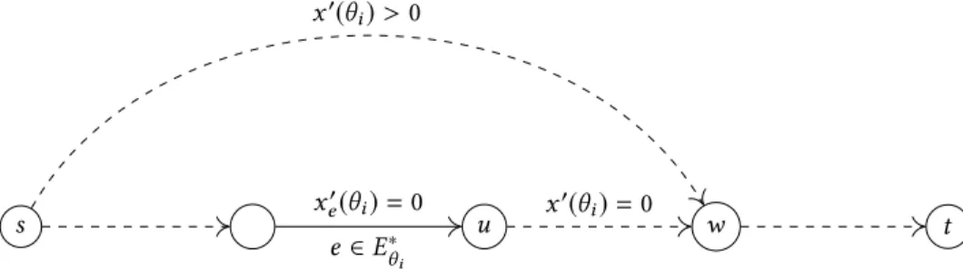
Proposition 7. In the dynamic equilibrium, for allθ ≥ 0such thate = (v,w) ∈ E_θ^∗, we have x_e^′(θ)>0, and hence, bothℓ_v^′(θ)>0andℓ_w^′(θ)>0.

s x u w t x^′(θi)>0

e∈E^∗_θi

x_e^′(θi)=0 x^′(θi)=0

Fig. 2. An illustration to clarify the proof of Proposition 7.

Proof. We prove the proposition by contradiction. We refer to Fig. 2 for an illustration of the proof.

Consider the earliest phaseiof the dynamic equilibrium such that there is an edgeesatisfying that for all timesθin phasei,e ∈E^∗_θ butx_e^′(θ)=0.⁵Because of our assumption thatiis the earliest such phase, we can assume thatx_e^′(θ^′)>0 forθ^′in phasei−1. Indeed, otherwisex_e^′(θ^′)=0 and the queue inedid not increase, soe∈E^∗_θ′, contradicting the assumption thatiis the earliest.

Letθi be the starting time of phasei. Sincex_e^′(θ^′)>0 forθ^′in phasei−1, there exists some active⁶s,t-pathpcontaininge. Of course,pis still active by timeθi.

Without loss of generality we can assume thateis the last edge (in the order induced byp) with the property of having a queue but not carrying flow in phasei, i.e,e ∈E^∗_θ

i andx_e^′(θi)=0. Let u∈V be the head ofe. Sincex_e^′(θi)=0 ande ∈E_θ^∗

i, thin flow condition (6) imposes thatℓ_u^′(θi)=0.

Moreover, all verticesv coming afterualongp that do not receive any flow would still satisfy ℓ_v^′(θi)=0. Thus considerw, the first vertex afterealongpreceiving some flow (possiblyw =t).

Note that this vertex does not receive flow frompasedoes not carry flow. The latter implies that ℓ_w^′(θi)=0 by the thin flow conditions (4) or (6). On the other hand, aswreceives flow from some edge outsidep, the thin flow conditions (5) or (6) imply thatℓ_w^′(θi)>0. A contradiction.

Therefore,x_e^′(θi)>0 and by Proposition 6, alsoℓ_v^′(θi)>0 andℓ_w^′(θi)>0. This extends to anyθ

in phaseibecause the derivatives are constant in a phase.

Finally, we will use the following proposition.

Proposition 8. ^log(x)_x ≤ ¹_efor allx >0.

Proof. Consider the function f(x) =log(x)/x forx > 0. Then f^′(x) =(1−log(x))/x², and clearlyf^′(x)>0 forx ∈ (0,e)andf^′(x)<0 forx∈ (e,+∞). Sox=e is the global maximum off

and the lemma follows sincef(e)=1/e.

We are now ready to state the two main lemmata that together form the heart of the proof of Theorem 2. The following lemma relates the completion time of the optimal flow and the equilibrium flow. It assumes the inflow rate of the optimum flow and the equilibrium flow are equal.

Lemma 9. IfuOPT =uEQ, the completion time of the optimal flowTOPT and of the equilibriumTEQ

are related as follows.

T_EQ−T_OPT ≤ 1 uEQ

Õ

e=(v,w)∈E

z_e(ℓ_v(θ))ˆ . (7)

5Note thatx^′is constant within a phase.

6By active we mean that all edges inpare inE^′_θ′.

Proof. Consider a path decompositionPof the optimal flow. From the linear program (3), it follows thatM =uOPTTOPT −Í

p∈ Pfˆpτp, whereτp =Í

e∈pτe. Moreover, from the equilibrium flow we knowM=u_EQθˆ. Therefore,

uOPTTOPT −uEQθˆ= Õ

p∈ P

fˆpτp. (8)

We will rewrite the right-hand side as follows. Note that for an edgee = (v,w) ∈ E,ℓ_w(θ) ≤ ℓ_v(θ)+ze(ℓ_v(θ))/νe+τeand henceτe ≥ℓ_w(θ) −ℓ_v(θ) −ze(ℓ_v(θ))/νe. Consider a pathp, summing over all edgese ∈pgivesτp ≥ℓ_t(θ) −ℓ_s(θ) −Í

e∈pze(ℓ_v(θ))/νe. Applying this inequality forθ=θˆ to Eq. (8) and using thatℓ_t(θˆ)=TEQ yields

uOPTTOPT −uEQθˆ≥Õ

p∈ P

fˆp©

­

«

TEQ−θˆ− Õ

e=(v,w)∈p

ze(ℓ_v(θˆ)) νe

ª

®

¬

. (9)

Because of our assumption,Í

pfˆp=uOPT =uEQ. Taking this out of the sum for the first two terms, we get

uOPTTOPT −uEQθˆ≥uEQTEQ−uEQθˆ−Õ

p∈ P

fˆp

Õ

e∈p

ze(ℓ_v(θ))ˆ νe , and hence,

uEQTEQ−uOPTTOPT ≤Õ

p∈ P

fˆp

Õ

e∈p

ze(ℓ_v(θˆ)) νe

=Õ

e∈E

fˆez_e(ℓ_v(θ))ˆ νe

≤Õ

e∈E

ze(ℓ_v(θˆ)).

The equality follows by summing over all edges instead of all paths, and the last inequality is implied byfˆe ≤νe. The result follows from our assumption thatuOPT =uEQ. To complete the proof of Theorem 2, it remains to bound the sum in the right-hand side of Eq. (7).

The following lemma does exactly this and does not rely on any assumption.

Lemma 10. In the dynamic equilibrium, for allθ ≥0, Õ

e=(v,w)∈E

ze(ℓ_v(θ)) ≤ uEQ

e (ℓ_t(θ) −ℓ_t(0)). We prove this lemma using two more technical claims.

Claim11. In the dynamic equilibrium, for allθ ≥0, Õ

e=(v,w)∈E

ze(ℓ_v(θ))=∫ θ 0

Õ

e=(v,w)∈E^′_ξ

x_e^′(ξ)

1− ℓ_v^′(ξ) ℓ_w^′(ξ)

dξ.

Proof of Claim 11. Unless indicated otherwise, by an edgeewe mean an edgee=(v,w). We begin by writing the queue length in terms of its derivative by using Eq. (1).

Õ

e=(v,w)∈E

ze(ℓ_v(θ))=Õ

e∈E

∫ θ 0

dze(ℓ_v(ξ))

dξ 1z_e(ℓ_v(ξ))>0dξ =∫ θ 0

Õ

e∈E^∗_ξ

dze(ℓ_v(ξ))

dξ dξ. (10)

Denoting the flow underlying the dynamic equilibrium byf, fore ∈E^∗_ξwe havez_e^′(ξ)=f_e⁺(ξ) −νe

andℓ_w^′(ξ)=x_e^′(ξ)/νe. Then, using Proposition 7, for edgese∈E^∗_ξ we can write dze(ℓ_v(ξ))

dξ =z_e^′(ℓ_v(ξ))ℓ_v^′(ξ)

=f_e⁺(ℓ_v(ξ))ℓ_v^′(ξ) −νeℓ_v^′(ξ)

=x_e^′(ξ) −νeℓ_v^′(ξ)

=x_e^′(ξ)

1−ν_eℓ_v^′(ξ) x_e^′(ξ)

=x_e^′(ξ)

1−ℓ_v^′(ξ) ℓ_w^′(ξ)

. Plugging the above expression into Eq. (10) yields

Õ

e∈E

ze(ℓ_v(θ))=∫ θ 0

Õ

e∈E^∗_ξ

x_e^′(ξ)

1−ℓ_v^′(ξ) ℓ_w^′(ξ)

.

Note that for edgese=(v,w) ∈E_ξ^′\E^∗_ξ, we haveℓ_w(ξ)=ℓ_v(ξ)+ze(ℓ_v(θ))/νe+τe, soℓ_w^′(ξ)=ℓ_v^′(ξ)+ z_e^′(ℓ_v(θ))ℓ_v^′(θ)/νe =ℓ_v^′(ξ)+0 almost everywhere. Using Proposition 6, this gives 1−ℓ_v^′(ξ)/ℓ_w^′(ξ)=0 almost everywhere, and hence

Õ

e∈E

ze(ℓ_v(θ))=∫ θ 0

Õ

e∈E^′_ξ

x_e^′(ξ)

1− ℓ_v^′(ξ) ℓ_w^′(ξ)

dξ.

The next claim bounds the integral on the right-hand side.

Claim12. In the dynamic equilibrium, for almost allξ ≥0, Õ

e=(v,w)∈E^′_ξ

x_e^′(ξ)

1−ℓ_v^′(ξ) ℓ_w^′(ξ)

≤uEQ·log(ℓ_t^′(ξ)),

Proof of Claim 12. Consider a path decompositionPof the dynamic equilibriumf at timeξ. Then we can rewrite the left-hand side as

Õ

e∈E_ξ^′

x_e^′(ξ)

1− ℓ_v^′(ξ) ℓ_w^′(ξ)

= Õ

p∈ P

x_p^′(ξ)Õ

e∈p

1− ℓ_v^′(ξ) ℓ_w^′(ξ)

.

Because of Proposition 6, we can apply the fact that 1−x ≤log(1/x)forx =ℓ_v^′(ξ)/ℓ_w^′(ξ) >0.

Therefore,

Õ

p∈ P

x_p^′(ξ)Õ

e∈p

1−ℓ_v^′(ξ) ℓ_w^′(ξ)

≤Õ

p∈ P

x_p^′(ξ)Õ

e∈p

log ℓ_w^′(ξ)

ℓ_v^′(ξ)

. Now rewrite log

_ℓ′ w(ξ) ℓ_v^′(ξ)

as log(ℓ_w^′(ξ)) −log(ℓ_v^′(ξ)). This gives a telescopic sum for every pathp∈ P, soÍ

e∈plog _ℓ′

w(ξ) ℓ_v^′(ξ)

=log(ℓ_t^′(ξ)) −log(ℓ_s^′(ξ)). Using thatℓ_s^′(ξ)=1 and thatx^′(ξ)is a flow of size uEQ, this yields

Õ

p∈ P

x_p^′(ξ)Õ

e∈p

log ℓ_w^′(ξ)

ℓ_v^′(ξ)

≤ Õ

p∈ P

x_p^′(ξ)log(ℓ_t^′(ξ))=uEQlog(ℓ_t^′(ξ)).

We now show how Lemma 10 follows from these claims.

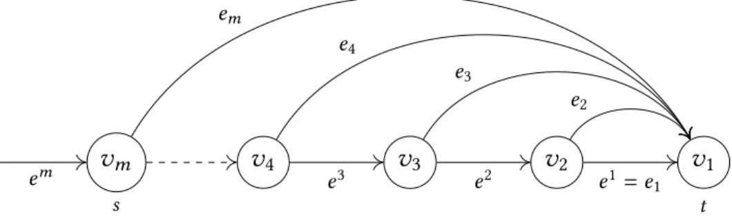
v

s

v

v

v

v

t

v

v

e^m e³ e² e¹=e¹

e_m

e4

e3

e2

Fig. 3. An illustration of the tight instance.

Proof of Lemma 10. From Claim 11 and Claim 12 we see that Õ

e=(v,w)∈E

ze(ℓ_v(θ)) ≤uEQ

∫ θ 0

log(ℓ_t^′(ξ))dξ. (11) Now substitute the monotonic functionξ =ℓ_t⁻¹(φ), giving dξ =_ℓ^{′ dφ}

t(l⁻¹(φ)). Then Eq. (11) becomes Õ

e∈E

ze(ℓ_v(θ)) ≤uEQ

∫ ℓ_t(θ) ℓt(0)

log ℓ_t^′ ℓ_t⁻¹(φ) ℓ_t^′ ℓ⁻¹_t (φ) dφ. We now apply Proposition 8 withx =ℓ_t^′ ℓ⁻¹_t (φ) >0 to see that

Õ

e∈E

ze(ℓ_v(θ)) ≤uEQ

∫ ℓt(θ) ℓt(0)

1 e

dφ=uEQ

e

(ℓ_t(θ) −ℓ_t(0)).

Theorem 2 follows in a straightforward manner from the two main lemmata above.

Proof of Theorem 2. Applying Lemma 10 forθ =θˆto the bound of Lemma 9 yields T_EQ−T_OPT ≤ 1

e

(ℓ_t(θ) −ˆ ℓ_t(0)) ≤ 1 e

ℓ_t(θ)ˆ .

The result follows by writingTEQ=ℓ_t(θˆ)and rearranging this inequality to ^TEQ

TO PT ≤ _e−1^e . The fact that this is tight follows from Lemma 15 in the next subsection.

3.1 Tightness

Consider the family of instances described in [18, Section 7.4], where it is proved that the Price of Anarchy of these instances is at most ^e

e−1. We will prove that for a given choice of the edge capacities, the Price of Anarchy of these instances tends to ^e

e−1 in the limit, thereby proving tightness.

For completeness, we describe the family of instances here, and they are illustrated in Fig. 3.

Fix parametersm ∈ Nandα >0. Denote the capacity of edgeei andeⁱ respectively byui and uⁱ = Íi

k=1ui. Set the delay ofei andeⁱ toτi =αu^m

1 uO PT −_u¹_i

andτⁱ =0, respectively. The equilibrium inflow rate isu^m.

We consider the instance where we setu¹ =1 anduⁱ = ^m_m⁻¹−2

i−1

. Note that this is a feasible choice as it is strictly increasing ini, and thereforeui >0. We set the total amount of flow to send through the network toM=αu^m.

The following lemmata show that the Price of Anarchy for this instance tends to ^e

e−1form→ ∞.

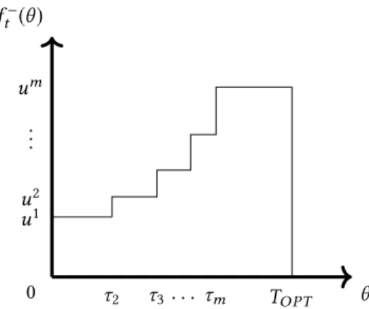
θ f_t⁻(θ)

0 u¹ u² ... u^m

τ² τ³. . . τm TOPT

Fig. 4. The inflow rate intotof the optimum flow for the tight instance.

Lemma 13. The completion time of the equilibrium isTEQ =αu^m.

Proof. Sinceτⁱ =0 for alli, the total delay of the straight path is 0. Therefore, in the first phase of the equilibrium, all particles take the straight path and we get

x_e^′= (

0 forei i=2, . . . ,m

u^m foreⁱ i=1, . . . ,m , and ℓ_v^′_i =u^m

uⁱ fori=1, . . . ,m. This yields

ℓ_v^′

1−ℓ_v^′_i = u^m

u¹ −u^m uⁱ

=τi

α for alli,

and therefore the first phase lasts until timeθ=α, when all paths enter the dynamic shortest path network. Since the equilibrium inflow rate isu^m, we haveθˆ=_u^Mm =α. Therefore,

TEQ =ℓ_t(θ)ˆ =ℓ_t(α)=α+τm =α+αu^m 1− 1

u^m

=αu^m.

Lemma 14. The completion time of the optimum flow isTOPT =τm.

Proof. See Fig. 4 for an illustration off_t⁻(θ), the inflow rate intotof the optimum flow as a function ofθ. Note that sinceMequals the area under this curve,

M=

m−1

Õ

i=1

(τ_i+¹−τi)uⁱ +(TOPT −τm)u^m.

Now observe that for alli=1, . . . ,m−1, (τ_i+1−τ_i)uⁱ =αu^m

1 uⁱ − 1

uⁱ⁺¹

uⁱ =αu^m 1− uⁱ

uⁱ⁺¹

=αu^m 1− m−1

m−2 ⁻¹!

= αu^m m−1

. We conclude that at timeτm, a total amount of flow of(m−1)^αu_m−1^m =αu^mhas arrived att. Since

M=αu^m, thereforeTOPT =τm.

Lemma 15. The Price of Anarchy of _e−1^e is tight.