ECOLE DOCTORALE D’ASTRONOMIE ET D’ASTROPHYSIQUE D’ÎLE-DE-FRANCE

UNIVERSITÄT ZU KÖLN – I. PHYSIKALISCHES INSTITUT MATHEMATISCH – NATURWISSENSCHAFT FAKULTÄT

&

OBSERVATOIRE DE PARIS – LERMA

ECOLE DOCTORALE D’ASTRONOMIE ET D’ASTROPHYSIQUE D’ÎLE-DE-FRANCE

PhD Thesis

To obtain the degree of Doctor

Author:

STÉPHAN Gwendoline

Modeling chemistry in massive star forming regions with internal PDRs

Supervisors:

Prof. Dr. SCHILKE Peter / Prof. Dr. LE BOURLOT Jacques

Defense: 4 ^th November, 2016

Members of the jury

Prof. Dr. WOLF Sebastian (Referee)

Dr. DESPOIS Didier (Referee)

Prof. Dr. SAUR Joachim (President)

Prof. Dr. SCHILKE Peter (Supervisor)

Prof. Dr. LE BOURLOT Jacques (Supervisor)

Prof. Dr. BOCKELÉE MORVAN Dominique (Member)

Prof. Dr. PINEAU DES FORÊTS Guillaume (Member)

Dr. SÁNCHEZ-MONGE Álvaro (Member)

Modeling chemistry in massive star forming regions with internal PDRs

INAUGURAL – DISSERTATION zur

Erlangung des Doktorgrades

der Mathematisch – Naturwissenschaftlichen Fakultät der Universität zu Köln

vorgelegt von

Gwendoline Stéphan

aus Pont l’Abbé

Köln 2016

Berichterstatter: Prof. Dr. SCHILKE Peter

Prof. Dr. WOLF Sebastian

Prof. Dr. DESPOIS Didier

Tag der mündlichen Prüfung: 4 ^th November, 2016

THÈSE DE DOCTORAT

de l’Université de recherche Paris Sciences et Lettres PSL Research University

Préparée dans le cadre d’une cotutelle entre Observatoire de Paris – LERMA

Universität zu Köln – I. Physikalisches Institut

Modeling chemistry in massive star forming regions with internal PDRs

Modélisation de la chimie dans les régions de formation d’étoiles massives avec PDRs internes

École Doctorale n ^o 127

École Doctorale d’Astronomie et d’Astrophysique d’Île-de-France Spécialité: Astronomie et Astrophysique

soutenue par Gwendoline STÉPHAN le 4 novembre 2016

dirigée par

Prof. Dr. Peter SCHILKE & Prof. Dr. Jacques LE BOURLOT

À ma famille et à son tout nouveau membre, Éléanore

“When walking through the ‘valley of shadows’, remember, a shadow is cast by a Light”

Austin O’Malley

Acknowledgements

This work was supported by the Collaborative Research Centre 956, sub-project Astro- chemistry [C3], funded by the German Deutsche Forschungsgemeinschaft (DFG), by the French CNRS national program PCMI (Physique et Chimie du Milieu Interstellaire) and by the COST Action CM1401 (European Cooperation in Science and Technology).

For this work, I used the Lapack and Blas Fortran libraries as well as several Python packages: numpy, astropy, matplotlib, pp and scipy. For the parallel jobs I also used the free software GNU parallel and some plots were generated with the command-line tool gnuplot. Furthermore, I made use of the following visualization softwares: ds9, kvis and Paraview. For the debugging and optimization of Saptarsy I used the application performance analyzer and visualizer Instruments integrated in environment Xcode.

Now, I would like to thank personally all the people who helped me to carry out this work and supported me during these four years.

First, I thank my supervisors Peter Schilke and Jacques Le Bourlot for their advice, for pushing me to be more accurate in my thinking and widening my view. Your assistance and the discussions we had were not just helpful but also necessary for me to improve the results and move forward. Despite your busy schedule and the distance, you always have been available to sit/skype with me when needed. I am very grateful you introduced me to the astrochemistry field and gave me the opportunity to pursue this very interesting research. I would also like to thank both of you for accepting this co-tutelle which was not easy to set up and had a few hick-ups on the way but end up to be very useful for me.

Second, I would like to thank my colleagues and collaborators: Rumpa Choudhury and Benjamin Godard (astrochemistry and Saptarsy), and Anika Schmiedeke (Pandora and RADMC-3D). This work would not have been possible without you developing the tools I used and helping me improving/optimizing them. Rumpa, you spent a lot of time at the beginning of my thesis explaining astrochemistry and how Saptarsy works. Benjamin, you were always there to answer the questions I had when I was in Paris and your help and advice on the optimization of Saptarsy was significant. Anika, thank you for spending so much time with me explaining Pandora, for helping me to implement new parts necessary for my work, for meeting with me or answering all my e-mails when I had questions, even silly ones or the ones I had already asked months before, and for giving me a lot of useful tips.

i

I also thank all the other people of my amazing working groups:

• German: Philipp Carlhoff, Claudia Comito, Ümit Kavak, Fanyi Meng, Thomas Möller, Stefan Pols, Sheng Li Qin, Mahya Sadaghiani, Álvaro Sánchez-Monge, Dirk Schae- fer, Sarah Segieth, Sümeyye Suri, Alexander Zernickel.

With a special and big thanks to Álvaro Sánchez-Monge and Sümeyye Suri who supported me, listened to me and answered all my questions.

• French: Emeric Bron, Frank Le Petit, Evelyne Roueff in the ISM team as well as David Languignon, Nicolas Moreau in the computer science team.

I am thankful to Cornelis Dullemond for the useful meetings and discussions we had on RADMC-3D and how to improve my models; Takashi Hosokawa for providing the stellar parameters data necessary to this work and answering my questions related to them; and Dmitry Semenov for sending me the results of the different models needed for benchmarking the codes.

I am really grateful to Frank Schlöder who was there to fix my laptop issues or com- puting problems and gave important tips which made the work much faster. I want to acknowledge the great assistance I received from Bettina Krause to deal with all the ad- ministrative paperwork required by the university when I started and later during these four years. I also want to thank Sebastian Haid who did the german translation of the abstract and save me a lot of my time. A two hours task for him would have been more than a day for me.

I am grateful to my SFB thesis committee members Stefan Schlemmer and Sandra Brüncken for the time they spent on the meetings and their advice; to the SFB students for their support and suggestions given during the student seminars as well as for the nice times spent during the student retreat; to the SFB coordinators Susanne Herbst and Maxi Limbach who helped in the organization of the the SFB thesis committee meetings.

Thank you to all my friends, students and post-docs, with whom I spent amazing lunches, tea times, dinners in Borsalino and excursions around Cologne: Sümeyye, Anika, Álvaro, Mahya, Pavol, Cristian, Daniel, Sebastian, Annika, Gerold, Nastaran, Prabesh, Elaheh, Anna, Michal, Philipp, Norma, Silke.

Special thanks to: Quang Nguyen-Luong who supported me in my research of a PhD position and suggested to apply for a job with Peter in Cologne; Christine Kuch who helped during these short coaching sessions to become more confident and more comfort- able during presentations.

Derniers mais pas les moindres, je remercie ma famille, et plus particulièrement mes

parents et mon frère. Vous avez toujours été là pour moi, vous m’avez poussé à atteindre

ce but et m’avez supporté tout le long du chemin. L’astrophysique serait demeuré juste

un rêve sans vous dans ma vie. Et je tiens aussi à remercier mes amies, Naïk, Charlotte,

Anna et Audrey, and of course Sümeyye. Vous avez toujours cru en moi et même si à

cause de la distance il n’a pas toujours été facile de garder le contact, tous les moments

passés avec vous ont été inoubliables.

Abstract

Title Modeling chemistry in massive star forming regions with internal PDRs

Keywords Astrochemistry: Chemical evolution

Massive star formation: HC/UCH II regions – Hot molecular cores – Photodissociation regions

Over the past decades star formation has been a very attractive field because knowl- edge of star formation leads to a better understanding of the formation of planets and thus of our solar system but also of the evolution of galaxies. Conditions leading to the formation of high-mass stars are still under investigation but an evolutionary scenario has been proposed: As a cold pre-stellar core collapses under gravitational force, the medium warms up until it reaches a temperature of 100 K and enters the hot molecular core (HMC) phase. The forming central proto-star accretes materials, increasing its mass and lumi- nosity and eventually it becomes sufficiently evolved to emit UV photons which irradiate the surrounding environment forming a hyper compact (HC) and then a ultracompact (UC) H II region. At this stage, a very dense and very thin internal photon-dominated region (PDR) forms between the H II region and the molecular core.

Information on the chemistry allows to trace the physical processes occurring in these different phases of star formation. Formation and destruction routes of molecules are influenced by the environment as reaction rates depend on the temperature and radiation field. Therefore, chemistry also allows the determination of the evolutionary stage of astrophysical objects through the use of chemical models including the time evolution of the temperature and radiation field.

Because HMCs host a very rich chemistry with high abundances of complex organic molecules (COMs), several astrochemical models have been developed to study the gas phase chemistry as well as grain chemistry in these regions. In addition to HMCs models, models of PDRs have also been developed to study in particular photo-chemistry. So far, few studies have investigated internal PDRs and only in the presence of outflows cavities.

Thus, these unique regions around HC/UCH II regions remain to be examined thoroughly.

My PhD thesis focuses on the spatio-temporal chemical evolution in HC/UC H II regions with internal PDRs as well as in HMCs. The purpose of this study is first to understand the impact and effects of the radiation field, usually very strong in these regions, on the chemistry. Secondly, the goal is to study the emission of various tracers of HC/UCH II regions and compare it with HMCs models, where the UV radiation field does not impact the region as it is immediately attenuated by the medium. Ultimately we want to determine the age of a given region using chemistry in combination with radiative transfer.

v

To investigate these transient phases of massive star formation, we use the astrochemi- cal code Saptarsy, optimized and improved during this PhD thesis. Saptarsy is a gas-grain code computing the spatio-temporal evolution of relative abundances. It is based on the rate equation approach and uses an updated Ohio State University (OSU) chemical net- work. Moreover, Saptarsy works along with the radiative transfer code RADMC-3D via a Python based program named Pandora. This is done in order to obtain synthetic spec- tra directly comparable to observations using the detailed spatio-temporal evolution of species abundances.

To summarize the Pandora framework: We use RADMC-3D to self-consistently com- pute the spatio-temporal evolution of the dust temperature and mean intensity of the radiation field adopting first, a model of accreting high mass proto-star which gives the time evolution of the stellar luminosity and second, a Plummer-like function as the density radial profile. Based on these parameters and initial conditions obtained with Saptarsy for a pre-stellar core model, Saptarsy computes the evolution of relative abundances which are next used by RADMC-3D to produce time-dependent synthetic spectra assuming Lo- cal Thermodynamic Equilibrium (LTE). These spectra can then be post-processed, i.e.

convolved to the beam of the observations we want to compare them with.

In addition to comparing a HC/UCH II region to a HMC model, we analyze models with different sizes of H II regions, with various densities at the ionization front as well as with two different density profiles. We investigate the critical dependance of the abundances on the initial conditions and we also explore the importance of the emission coming from the envelope for various species. We find that among the dozen of molecules and atoms we have studied only four of them trace the UC/HCH II region phase or the HMC phase.

They are C

and O for the first and CH

OH and H

O for the second phase. However,

more species could be studied to probe and identify these phases. For instance, CO

seems a good candidate to trace PDRs but it is not abundant enough in our model. It

appears that models including an outflow cavity produce more of this molecule. Thus,

we could modify the geometry of our source structure by adding an outflow, and later

even more complex geometries. More improvements could also be made such as simple

computation of the gas temperature in Saptarsy which might strongly affect the chemistry

inside the PDR.

Zusammenfassung

Titel Chemische Modellierung in massereichen Sternentstehungsgebieten durch interne PDRs Schlüsselwörter Astrochemie: Chemische Evolution

massereiche Sternentstehung: HC/UCH II Regionen – Heiße molekulare Kerne – Photodissoziationsregionen

Während der letzten Jahrzehnte hat die Bedeutung des Forschungsgebiets der Ster- nentstehung stark zugenommen. Das Wissen darüber liefert ein besseres Verständnis über die Entstehung von Planeten, des Sonnensystems und der Entwicklung von Galaxien. Ob- wohl die genauen Bedingungen für die Entstehung von massereichen Sternen noch unter- sucht werden müssen, kann trotzdem ein grundsätzliches Szenario angenommen werden:

Unter dem Einfluss der Gravitation kollabiert der kalte Vorgänger eines Sterns. Dabei erwärmt sich dieser bis auf Temperaturen von ungefähr 100 K und geht in die "heiße molekulare Phase" (HMC) über. Der entstehende Protostern akkretiert Material, wächst somit in Masse. Ist der Stern hinreichend entwickelt beginnt er UV Strahlung zu emit- tieren. In der beschienene Umgebung bildet sich eine hyperkompakte (HC) und dann ultrakompakte (UHC) H II Region aus. Zwischen der H II Region und dem molekularen Kern bildet sich eine dichte, dünne interne photonen-dominierte Region (PDR) aus.

Die chemische Information kann Aufschluss geben über die physikalischen Prozesse der verschiedenen Phasen der Sternentstehung, da Reaktionsraten durch die Temperatur und das Strahlungsfeld des Umfeld bestimmt werden. Die Chemie und deren zeitliche Mod- ellierung erlaubt dadurch eine Bestimmung des Entwicklungsstandes von astrophysikalis- chen Objekten.

HMCs weisen eine komplizierte chemische Zusammensetzung auf mit einem hohen Anteil an komplexen organischen Molekülen (COM). Um die Gasphasen- und Staub- Chemie in den angesprochenen Gebieten zu untersuchen wurden mehrere astrochemische Modelle entwickelt. Hinzu kommen spezielle Modelle, die sich mit der Photochemie in PDRs beschäftigen. Nur wenige Arbeiten zielen auf interne PDRs ab und das meist nur in Gebieten mit geringer Dichte, welche durch die Gegenwart von Ausflüssen entstanden sind. Die einzigartigen HC/UCH II Regionen müssen noch gründlicher erforscht werden.

Meine Doktorarbeit beschäftigt sich mit der chemischen Entwicklung in HC/UCH II Regionen durch interne PDRs und HMCs. Ein Ziel dieser Arbeit ist das grundsätzliche Verständnis wie das Strahlungsfeld auf die Chemie Einfluss nimmt. Es soll die Emission unterschiedlicher Tracer in HC/UCH II Regionen erklärt und mit dem HMC Model, in denen das UV Strahlungsfeld sofort abgeschwächt wird, verglichen werden. Letztendlich möchte ich das Alter einer gegeben Region mit Hilfe von Chemie und Strahlungstransfer- Simulationen bestimmen.

vii

Zur Untersuchung dieser kurzen Phase in der Sternentstehung benutze ich den astro- chemischen Code Saptarsy, welcher während der Dissertation verbessert und optimiert wurde. Saptarsy ist ein Gas-Staub Programm, welches die zeitliche und räumliche En- twicklung der relativen Häufigkeiten chemischer Spezies berechnet. Es basiert auf einen Ratengleichungsansatz und nutzt dazu ein -von der Ohio State University (OSU)- überar- beitetes chemischen Netzwerk. Zusätzlich arbeitet Saptarsy mit dem Strahlungstransfer Code RADMC-3D über eine Python basierende Schnittstelle, Pandora genannt, zusam- men. Schlussendlich ist es damit möglich, die erhaltenen synthetischen Spektren mit Beobachtungen zu vergleichen.

Eine kurze Zusammenfassung von Pandora: RADMC-3D berechnet selbst-konsistent die räumliche und zeitliche Entwicklung der Staubtemperatur und die mittlere Intensität des Strahlungsfeldes. Angenommen wird dazu ein Modell eines massereichen Proto-Sterns und desses Leuchtkraft sowie ein Plummer-Dichte-Profil. Mit diesen Parametern und den Anfangsbedingungen aus Saptarsy wird die Entwicklung der relativen Häufigkeiten berechnet. RADMC-3D erzeugt daraus zeitabhängige synthetische Spektren unter der Annahme eines lokalen thermodynamischen Gleichgewichts. Diese Spektren können nun mit dem zu beobachtenden Strahl gefaltet werden und sind somit mit Beobachtungen vergleichbar.

Zusätzlich werden Größen von H II Regionen bei unterschiedlicher Dichte der Ionisa-

tionsfront und bei zwei weiteren Dichteprofilen bestimmt. Es wird gezeigt, dass die An-

fangsbedingungen entscheidend sind für die chemische Häufigkeit von chemischen Spezies

und dass die Emission der Einhüllenden eine entscheidende Rolle spielt. Unter Dutzen-

den von Molekülen und Atomen, die die Phase in HC/UCH II oder der HMC beschreiben,

betrachten wir vier näher. Für die erste genannte sind dies C

und O sowie CH

OH

und H

O für die zweite. Weitere Spezies wären möglich. Als Beispiel hierfür sei CO

genannt. Jedoch weist diese Spezies in unserer Beschreibung eine zu geringe Häufigkeit auf

verglichen mit Modellen die auch Gebiete niedriger Dichte in Betracht ziehen. Zukünftig

sollte deswegen die ursprüngliche Geometrie angepasst werden. Eine weitere Verbesserun-

gen ergebe sich durch die direkte Berechnung der Gastemperatur in Saptarsy. Dadurch

könnte sich die Chemie in PDRs deutlich verändert werden.

Résumé

Titre Modélisation de la chimie dans les régions de formation d’étoiles massives avec PDRs internes

Mots clés Astrochimie: Evolution chimique

Formation d’étoile massive: Régions H II hypercompactes et ultracompactes – Cœurs chauds moléculaires – Régions de photodissociation

Au cours des dernières décennies, la formation des étoiles a été un sujet très attractif.

La connaissance de la formation des étoiles conduit à une meilleure compréhension de la formation des planètes, donc de notre système solaire mais également de l’évolution des galaxies. Les conditions menant à la formation des étoiles massives sont toujours étudiées mais un scénario de leur évolution a été avancé: lors de l’effondrement d’un cœur froid pré-stellaire sous l’effet de la gravité, le milieu se réchauffe jusqu’à atteindre une température de 100 K. Il entre ainsi dans la phase de cœur chaud moléculaire (CCM).

La proto-étoile centrale en formation accrète de la matière, augmentant sa masse et sa luminosité. Finalement elle devient suffisamment évoluée pour émettre des photons UV.

Ceux-ci irradient l’entourage de l’étoile formant ainsi une région H II hypercompacte (HC), puis une région H II ultracompacte (UC). À ce stade, une région de photo-dissociation (PDR) se forme entre la région H II et le cœur moléculaire.

La composition chimique du milieu nous permet de connaître les processus physiques ayant lieu pendant les différentes phases de la formation des étoiles. Les chemins de formation et de destruction des molécules sont influencés par l’environnement parce que les taux de réaction dépendent de la température et du champ de rayonnement. De plus, la chimie nous permet également de déterminer le stade de l’évolution d’un objet astrophysique par l’utilisation de codes chimiques incluant l’évolution temporelle de la température et du champ de rayonnement.

Plusieurs codes ont été développés afin d’étudier la chimie en phase gazeuse ainsi que la chimie de surface dans les cœurs chauds moléculaires. Ces régions abritent une chimie extrêmement riche avec de très fortes abondances pour les molécules organiques complexes. En plus des modèles de cœurs chauds, des modèles de PDRs ont été développés pour étudier notamment la photochimie. Jusqu’à présent, très peu d’études ont examiné les PDRs internes et cela a été fait uniquement en présence d’une cavité formée par un écoulement de matière depuis les pôles de la proto-étoile vers le milieu environnant (appelé ici outflow). La connaissance de ces régions uniques autour des régions H II hypercompact et ultracompact restent donc à approfondir.

Ma thèse de doctorat se concentre sur l’évolution spatio-temporelle de la chimie dans les régions H II hypercompact et ultracompact avec des PDRs internes ainsi que la chimie dans les cœurs chauds moléculaires. Premièrement, l’objectif de ce travail est de compren-

ix

dre l’impact et les effets sur la chimie du champ de rayonnement, en général très fort dans ces régions. Deuxièmement, le but est d’étudier l’émission de diverses espèces spécifiques aux régions H II HC/UC et de comparer cette émission à celle des CCMs, régions où le champ de rayonnement UV n’a pas d’influence vu qu’il est immédiatement atténué par le milieu. En fin de compte, nous voulons déterminer l’âge d’une région donnée en utilisant la chimie associée au transfert radiatif.

Pour étudier ces stades transitoires de la formation des étoiles massives, nous utilisons le code astrochimique Saptarsy optimisé et amélioré pendant cette thèse de doctorat.

Saptarsy est un code gaz-grain calculant l’évolution spatio-temporelle d’abondances rela- tives. Il est basé sur l’approche des équations des taux de réactions et il utilise le réseau chimique OSU (Université de l’État de l’Ohio) mis à jour. De plus, Saptarsy est couplé au code de transfert radiatif RADMC-3D via un programme, basé sur le langage Python, nommé Pandora, en vue d’obtenir des spectres synthétiques directement comparables avec des observations en utilisant l’évolution spatio-temporelle détaillée des abondances chimiques.

Pour résumer le fonctionnement de Pandora: nous utilisons RADMC-3D pour calculer de manière auto-cohérente l’évolution spatio-temporelle de la température des grains et de l’intensité du champ de rayonnement. Tout d’abord, nous adoptons un modèle de proto-étoile massive qui fournit l’évolution temporelle de la luminosité de l’étoile. Dans un deuxième temps, nous utilisons une fonction de Plummer pour définir le profil radial de la densité. Avec ces paramètres et des conditions initiales obtenues avec Saptarsy pour un modèle de cœur pré-stellaire, Saptarsy calcule l’évolution des abondances relatives.

Elles sont ensuite utilisées par RADMC-3D pour produire, dans l’approximation ETL (Équilibre Thermodynamique Local), des spectres synthétiques dépendant du temps. Ces spectres peuvent finalement être convolués afin qu’ils aient la même résolution que les observations avec lesquelles nous voulons les comparer.

En plus de la comparaison entre un modèle de région H II HC/UC et un modèle de CCM, nous comparons des modèles avec des tailles différentes de régions H II , avec plusieurs densités au front d’ionisation, ainsi qu’avec deux profils de densité différents.

Nous étudions les abondances qui dépendent de manière critique des conditions initiales et nous explorons aussi l’importance de l’émission venant de l’enveloppe pour diverses espèces chimiques. Nous constatons, parmi la douzaine d’espèces étudiées, que seulement quatre d’entre elles sont spécifiques à la phase de région H II ou à la phase de cœur chaud.

Ces espèces sont C

et O pour la première phase et CH

OH et H

O pour la deuxième phase. Cependant, un plus grand nombre d’espèces pourrait être utilisées pour étudier et identifier ces phases. Par exemple, CO

semble un bon candidat pour tracer des PDRs mais il n’est pas assez abondant dans notre modèle. Il semble que des modèles incluant une cavité produite par un «outflow» accroissent la production de cette molécule. Nous pourrions donc modifier la géométrie de la structure de la source en ajoutant un «outflow»

et ultérieurement, une géométrie bien plus complexe. D’autres améliorations pourraient

être apportées, tel un calcul simple de la température du gaz dans Saptarsy ce qui pourrait

fortement affecter la chimie à l’intérieur de la PDR.

Contents

1 Introduction 1

1.1 Interstellar medium . . . . 2

1.1.1 Interstellar medium cycle . . . . 2

1.1.2 Gas . . . . 2

1.1.3 Dust . . . . 4

1.2 Star formation . . . . 6

1.2.1 Theoretical star formation scenario(s) . . . . 7

1.2.2 Massive star formation: From an observational point of view . . . . 9

1.3 Chemistry in the ISM . . . . 11

1.3.1 Gas phase chemistry . . . . 12

1.3.2 Surface chemistry . . . . 13

1.3.3 Chemical models . . . . 16

1.4 About this work . . . . 17

1.4.1 Goal of the thesis . . . . 17

1.4.2 Approach and strategy . . . . 17

1.4.3 Organization of the thesis . . . . 18

I Codes 19 2 The chemical code: Saptarsy 21 2.1 What is Saptarsy? . . . . 22

2.1.1 Reactions and networks . . . . 22

2.1.2 Numerical solvers: DVODPK and MA28 . . . . 28

2.2 Improvements to model a H II region . . . . 29

2.2.1 Radiation field evolution . . . . 29

2.2.2 Logarithmic version . . . . 32

2.2.3 Interpolation: Temperatures and radiation field as variables . . . . 33

2.3 Benchmarking . . . . 34

2.3.1 Semenov code . . . . 34

2.3.2 TDR . . . . 35

3 Pandora 39 3.1 Dust temperature & radiation field computation . . . . 40

3.1.1 Luminosity evolution . . . . 41

3.1.2 Density and structure of the cores . . . . 43

3.1.3 Dust properties . . . . 45

3.2 Synthetic spectra . . . . 47

xiii

3.2.1 Line emission . . . . 47 3.2.2 Post-processing . . . . 48

4 Semi-analytical model 51

4.1 Equations Case 1 . . . . 52 4.2 Scaling . . . . 53 4.2.1 Length . . . . 53 4.2.2 Time . . . . 54 4.2.3 Logarithmic variables and Jacobian . . . . 55 4.3 Equations Case 2 . . . . 55 4.3.1 Grain properties . . . . 55 4.3.2 Evolution equations . . . . 56 4.3.3 Scaling . . . . 56 4.4 Sums . . . . 58 4.5 Integration . . . . 58 4.5.1 Discretization . . . . 58 4.5.2 Algorithm . . . . 59 4.5.3 Time step . . . . 59 4.6 Results . . . . 60 4.6.1 2D plots . . . . 60 4.6.2 Transition values . . . . 60

II Results 69

5 Models 71

5.1 Computation of the initial abundances . . . . 72 5.2 Selected species . . . . 74 5.3 Diagnostic tools . . . . 75 5.4 Hollow hot core vs Hot core . . . . 79 5.5 HC/UCH II region vs Hollow hot core . . . . 81 5.5.1 Size of the ionized cavity . . . . 83 5.5.2 Density at the ionization front . . . . 84 5.5.3 Plummer exponent . . . . 86

6 Results and analysis 89

6.1 Hollow hot core vs Hot core . . . . 91 6.2 H II region vs Hollow hot core . . . . 98 6.3 H II region size . . . 105 6.4 Density at the ionization front . . . 110 6.5 Plummer exponent . . . 115 6.6 Initial abundances . . . 117 6.7 Effect of the envelope . . . 123 6.8 Dissociation front . . . 127

7 Conclusions & Outlook 131

7.1 Conclusions . . . 131

7.2 Outlook . . . 134

xv

A Additional figures: Selected molecules 137

A.1 HC

N . . . 138 A.2 HN

C . . . 145 A.3 HCO . . . 155 A.4 HCO

. . . 165 A.5 H

CO . . . 175 A.6 CH

OH . . . 185 A.7 CN . . . 195 A.8 NH

. . . 205 A.9 N

H

. . . 215 A.10 H

O . . . 225 A.11 C . . . 235 A.12 C

. . . 245 A.13 O . . . 255 B Additional figures: abundance for other molecules 265 B.1 HMC vs HHMC model . . . 266 B.2 H II region size . . . 271 B.3 Density at the ionization front . . . 276 B.4 Plummer exponent . . . 281 B.5 Initial abundances . . . 286

C Dust spectral index in Sgr B2(N) 291

C.1 Introduction . . . 291 C.2 Data . . . 293 C.3 Determination of the dust spectral index . . . 294 C.3.1 First method: CH

OH a-type bands . . . 295 C.3.2 Second method: Optically thick CH

OH lines . . . 298

D Paper 301

List of Figures

1.1 Interstellar medium cycle . . . . 3 1.2 Dust grains structure . . . . 5 1.3 Dust life cycle . . . . 5 1.4 Low mass star formation scheme . . . . 7 1.5 High mass star formation scheme . . . . 9 1.6 Photon-dominated region scheme . . . . 11 1.7 Gas phase and dust surface’s reactions scheme . . . . 13 1.8 Scheme of Langmuir-Hinshelwood and Eley-Rideal mechanisms . . . . 15 2.1 H

self-shielding factor as a function of the H

column density . . . . 25 2.2 Example of the radiation field evolution as a function of radius . . . . 31 2.3 Benchmarking of Saptarsy: Semenov et al. (2010) – TMC–1 model . . . . 36 2.4 Benchmarking of Saptarsy: Semenov et al. (2010) – Hot core model . . . . 36 2.5 Benchmarking of Saptarsy: TDR model 1 . . . . 37 2.6 Benchmarking of Saptarsy: TDR model 2 . . . . 37 3.1 Flowchart of the modeling framework Pandora . . . . 40 3.2 Evolution of the stellar parameters M

, R

, L

and T

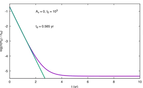
. . . . 42 3.3 Density profiles . . . . 44 3.4 Scheme of the H II region, hollow HMC and HMC models . . . . 44 3.5 Absorption and scattering efficiencies . . . . 45 3.6 Dependence of the dust temperature on the scattering and grain composition 46 3.7 Scheme of the ray-tracing in a AMR grid . . . . 49 4.1 Case 1: Spatio-temporal evolution of H

abundance . . . . 60 4.2 Case 2: Spatio-temporal evolution of adsorbed H abundance . . . . 61 4.3 Case 1 and 2: Time evolution of H

abundance at the edge of the cloud . 62 4.4 Case 1: H/H

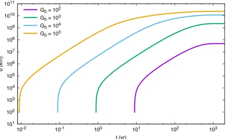
transition as a function of the radiation field . . . . 62 4.5 Case 1: Time evolution of the dissociation front position . . . . 63 4.6 Case 2: Time evolution of the dissociation front position for χ

= 10

. . . 64 4.7 Time evolution of the dissociation front velocity for several radiation fields 64 4.8 Case 1: Dissociation front final position as a function of radiation field . . 66 5.1 Diagnostic tool: Bacon plot . . . . 75 5.2 Diagnostic tool: Synthetic spectra . . . . 76 5.3 Diagnostic tool: Integrated intensity . . . . 77 5.4 Diagnostic tool: Integrated intensity ratio . . . . 78 5.5 Diagnostic tool: Integrated intensity ratio – ratio . . . . 78

xvii

xviii List of Figures 5.6 Scheme of the HMC and hollow HMC models . . . . 80 5.7 Hollow HMC vs HMC: Density and extinction profiles . . . . 80 5.8 Hollow HMC vs HMC: Spatio-temporal evolution of the temperature . . . 81 5.9 Scheme of the HC/UCH II region and hollow HMC models . . . . 82 5.10 HC/UCH II region vs Hollow HMC: Spatio-temporal evolution of the tem-

perature and radiation field . . . . 82 5.11 Size of the ionized cavity: Density and extinction profiles . . . . 83 5.12 Size of the ionized cavity: Spatio-temporal evolution of the temperature

and radiation field . . . . 84 5.13 Density at the ionization front: Density and extinction profiles . . . . 85 5.14 Density at the ionization front: Spatio-temporal evolution of the temper-

ature and radiation field . . . . 85

5.15 Plummer exponent: Density and extinction profiles . . . . 86

6.1 Scheme of the abundance regions in a H II region . . . . 91

6.2 Hollow HMC vs HMC: CH

OH relative abundance profile . . . . 92

6.3 Hollow HMC vs HMC: H

CO synthetic spectra . . . . 94

6.4 Hollow HMC vs HMC: HC

N, HN

C and CH

OH integrated intensities . 95

6.5 Hollow HMC vs HMC: Integrated intensity ratios . . . . 96

6.6 Hollow HMC vs HMC: Integrated intensity ratio – ratio . . . . 96

6.7 Scheme of the abundance regions in a H II region . . . . 98

6.8 H II region vs Hollow HMC: C

and CH

OH relative abundance profiles . 99

6.9 H II region vs Hollow HMC: H

CO synthetic spectra . . . 101

6.10 H II region vs Hollow HMC: HC

N and CH

OH integrated intensities . . 102

6.11 H II region vs Hollow HMC: Integrated intensity ratios . . . 102

6.12 H II region vs Hollow HMC: Integrated intensity ratio – ratio . . . 103

6.13 Size of the ionized cavity: H

O and HCN relative abundance profiles . . . 105

6.14 Size of the ionized cavity: H

CO synthetic spectra . . . 106

6.15 Size of the ionized cavity: HC

N and CH

OH integrated intensities . . . 107

6.16 Size of the ionized cavity: Integrated intensity ratios . . . 109

6.17 Size of the ionized cavity: Integrated intensity ratio – ratio . . . 109

6.18 Density at the ionization front: C

and CH

OH relative abundance profiles111

6.19 Density at the ionization front: H

CO synthetic spectra . . . 112

6.20 Density at the ionization front: HC

N and CH

OH integrated intensities 113

6.21 Density at the ionization front: Integrated intensity ratios . . . 113

6.22 Density at the ionization front: Integrated intensity ratio – ratio . . . 114

6.23 Plummer exponent: NH

relative abundance profiles . . . 115

6.24 Plummer exponent: HC

N and CH

OH integrated intensities . . . 116

6.25 Initial abundances: NH

and CH

OH relative abundance profiles . . . 118

6.26 Profile of the sum of the relative abundances of the main C-bearing species 119

6.27 Initial abundances: CN synthetic spectra . . . 120

6.28 Initial abundances: Integrated intensities . . . 121

6.29 Initial abundances: Integrated intensity ratios . . . 122

6.30 Initial abundances: Integrated intensity ratio – ratio . . . 123

6.31 Cut-off density: CN synthetic spectra . . . 124

6.32 Cut-off density: HC

N and N

H

integrated intensities . . . 125

6.33 Cut-off density: Integrated intensity ratios . . . 126

List of Figures xix

6.34 Cut-off density: Integrated intensity ratio – ratio . . . 126

6.35 Dissociation front: H

abundance profile . . . 127

List of Tables

1.1 Properties of the ISM phases . . . . 4 1.2 Properties of star formation regions . . . . 6 1.3 Types of H II region and their properties . . . . 10 1.4 Formation of methyl formate and dimethyl ether . . . . 12 1.5 List of the gas phase reactions . . . . 14 1.6 List of the grain surface reactions . . . . 15 1.7 Example of binding energies on bare grains and ice surface . . . . 16 2.1 List of the variables used in Saptarsy . . . . 27 2.2 List of the updated desorption energies . . . . 28 3.1 Phases of the evolution of the accreting massive proto-star. . . . 43 5.1 Initial abundances . . . . 73 5.2 Table of selected species . . . . 74 5.3 Abbreviations used for the integrated intensity ratios . . . . 79 5.4 Temperature and radiation field intensity values at 10

years for different

sizes of H II region . . . . 84 6.1 Abbreviations used for the models . . . . 90 6.2 Dissociation front position for all the models . . . 128

xxi

List of Abbreviations

AMR Adaptive Mesh Refinement

CNM Cold Neutral Medium

COM Complex organic molecules

CR Cosmic-Rays

DVODPK Differential Variable-coefficient Ordinary Differential equation solver with the Preconditioned Krylov method

FIR Far Infrared

FUV Far Ultraviolet

GMRES Generalized minimal residual method H II Ionized hydrogen

HCH II Hypercompact H II (region) HHMC Hollow Hot Molecular Core HMC Hot molecular core

HSL Harwell mathematical Software Library

IR Infrared

IGM Intergalactic medium ISM Interstellar medium

KH Kelvin-Helmholtz

KIDA KInetic Database for Astrochemistry LTE Local thermodynamic Equilibrium

MIR Mid-Infrared

MHD Magneto-hydrodynamical

NIR Near Infrared

OSU Ohio State University

PAH Polycyclic Aromatic Hydrocarbon

PDR Photon-dominated region / Photo-dissociation region TDR Turbulence Dissipation Region

UCH II Ultracompact H II (region)

UV Ultraviolet

WIM Warm Ionized Medium

WNM Warm Neutral Medium

xxiii

1

Introduction

Contents

1.1 Interstellar medium . . . . 2 1.1.1 Interstellar medium cycle . . . . 2 1.1.2 Gas . . . . 2 1.1.3 Dust . . . . 4 1.2 Star formation . . . . 6 1.2.1 Theoretical star formation scenario(s) . . . . 7 1.2.2 Massive star formation: From an observational point of view . 9 1.3 Chemistry in the ISM . . . . 11 1.3.1 Gas phase chemistry . . . . 12 1.3.2 Surface chemistry . . . . 13 1.3.3 Chemical models . . . . 16 1.4 About this work . . . . 17 1.4.1 Goal of the thesis . . . . 17 1.4.2 Approach and strategy . . . . 17 1.4.3 Organization of the thesis . . . . 18

Our galaxy, the Milky Way, is a spiral galaxy, of a total mass of 8×10

M (Peñarrubia et al. 2014), composed principally of stars (M

∼ 7×10

M ; Li & White 2009, McMillan 2011) and gas. Like other galaxies the Milky Way is a gravitationally bound astrophysical object in the shape of a disk and of a size of ∼ 20 kpc in length and ∼ 250 pc in height (Sparke & Gallagher 2000). Its different components interact with each other. One of its major components is the interstellar medium (ISM) containing gas that is slowly converted into stars as the Galaxy evolves. Gas can be ejected into the intergalactic medium (IGM)

1

2 Chapter 1. Introduction through galactic winds and can infall from the IGM as well. Most of the gas in the Galaxy is situated within a thin disk (≤ 500 pc; Dickey & Lockman 1990, Savage & Wakker 2009) where the majority of the stars populating the Galaxy are formed.

1.1 Interstellar medium

The medium between stars, the so called interstellar medium, is composed of a mixture of gas and dust and is a major component of galaxies. It represents only 10 – 15% of the mass of the Milky Way’s disk but the different processes taking place there such as motions, heating, cooling, etc. affect the matter as well as its physical and chemical state.

Furthermore, the ISM is an environment with a great variety of scales in size, temperature and also density despite it remains one of the less dense media of galaxies.

1.1.1 Interstellar medium cycle

The matter in the ISM is constantly renewed and enriched with heavy elements due to the cycle of star formation. This cycle can be described as follows (see also Fig. 1.1):

A diffuse cloud begins to collapse under the effect of gravity, fragments and form denser cores. Proto-stars form in these cold and dense cores through the accretion of the envelope.

Then, the proto-star rotation fastens and its surrounding cloud flatten up into an accretion disk. Proto-stars also eject material through bipolar outflows which show that the proto- star still accretes materials through the disk. Accretion stops once radiative pressure is strong enough to blow away the internal part of the disk. The remains are called a proto-planetary disk. Inside this disk the ice and dust accrete and aggregate to form planetesimals which then become planets or smaller objects like satellites. During their lifetime, stars modify their environment via photodissociation, ionization and heating.

Finally, the stars either shed their outer layers if they have a low mass and most of this mass is transferred back into the ISM or explode as supernovae at the end of their lifetime, i.e. when they have exhausted all their materials and are not able to hold fusion processes anymore. They eject newly formed heavy elements and heat the surrounding medium.

Then, this medium cools and disperses the material which is thus injected back into the ISM.

1.1.2 Gas

The gas is the main component of the ISM as it represents 99% of its mass (Hildebrand 1983). The interstellar gas is composed of hydrogen (90.8%) and helium (9.1%). The remaining percentage is heavier elements formed within the previous generations of stars.

In mass these percentages become: 70.4% of H, 28.1% of He and heavier elements 1.5%.

The gas can be atomic, molecular or ionized depending on the environment and the physi-

cal processes happening there. It is structured in different phases in constant interactions

1.1. Interstellar medium 3

Figure 1.1: Interstellar medium cycle. Image credit: Bill Saxton, NRAO/AUI/NSF

one with another.

Most of the gas is found in the atomic form, observable in the visible and UV range, and it can be divided into two phases. The first one, the Cold Neutral Medium (CNM), is a low density, neutral and cold medium (see Tab. 1.1). The second medium, the Warm Neutral Medium (WNM), has higher temperature and the same density as the CNM.

These two atomic phases can exist in a stable pressure equilibrium due to the cooling and heating mechanisms. The Warm Ionized Medium (WIM) has the same temperature as the WNM but a lower density and the hydrogen is ionized. This phase occupies a large volume given a volume filling factor of 0.25 (McKee & Ostriker 1977), although it is not the most voluminous. Other kinds of ionized gas regions exist such as hot interclouds and H II (ionized hydrogen) regions. Hot interclouds fill the largest volume and are extremely hot, T ∼ 10

K. As for H II regions they have a typical temperature of 10

K (Peimbert 1967;

Wilson et al. 2015) and a density n

(= n(H) + 2n(H

)) spreading from 1 to 10

cm

. They undergo expansion as they are not confined by their own gravity or by the gravity of the stars they contained and external pressure is insufficient to confine them. This is not the case of molecular clouds which are self-gravitating objects occupying only a small fraction of the ISM volume. Molecular clouds are mainly composed of molecular hydrogen. Molecular clouds have a temperature inferior to 100 K and a density superior to 5×10

cm

. It is within molecular clouds that star formation happens.

Dividing the gas phase into these phases is a conventional, but probably too simple, vision of the ISM. H I observations suggest that a significant amount of the atomic gas has a temperature between the CNM and WNM phases and thus is in the thermally unstable regime (500 ≤ T

≤ 5000 K – T

is the kinetic temperature; Heiles & Troland 2003; Roy et al. 2013). The thermal instability of the gas is a major physical process inducing turbulence in the ISM along with supernovae feedback, stellar winds or bipo- lar outflows. The interaction between magneto-hydrodynamical (MHD) turbulence and thermal instability might drive the formation of dense structures in molecular clouds. For example, Miville-Deschênes et al. (2016) suggests that dense structures in the Draco Neb- ula originate from the collision of diffuse gas which triggers the transition from WNM to CNM via the H I thermal instability because of the compression and increase in density of the WNM. This scenario was also proposed by several numerical simulations, e.g. Saury et al. (2014). Same properties of dense structures are found in other molecular clouds.

MHD simulations show also than turbulence acts to mix the different phases of the ISM

4 Chapter 1. Introduction Table 1.1: Characteristics of the different phases of the ISM in the Milky Way. The given number are approximations (Tielens 2005; Draine 2011).

Phase Temperature (K) Density n

(cm

) Total mass (M )

CNM 100 5×10

1.5×10

WNM 8000 5×10

1.5×10

WIM 8000 10

10

H II regions 10

1 – 10

5×10

Hot interclouds 10

0.005 10

Molecular clouds < 100 > 500 1.5×10

(Seifried et al. 2011).

1.1.3 Dust

Despite the fact that dust grains represent a very low percentage in mass of the ISM they are a very important component of it. Indeed, they play an essential role in the spectral energy distribution in the Galaxy. They are the main shield against low energy non ionizing photons with energies ranging in the visible and near/mid-infrared (NIR/MIR) spectrum. Dust grains scatter starlight efficiently, even more when they are fluffy and porous despite the low abundances of this kind of grains (Boulanger et al. 1996; Smith

& Dwek 1998). They also absorb almost half of the photons in the ultraviolet (UV) and visible spectra of the Galaxy, and then reradiate them in IR and sub-millimetric (sub-mm) range. It seems that ∼ 30% of the emitted starlight is reradiated by dust in the infrared (Bernstein et al. 2002).

Dust grains, precursors of solar system solids, possess different morphologies and com- position which can be deduced from absorption and emission (Draine 2003; Draine &

Li 2007). Their size spans from ∼ 1 nm to ∼ 1 µm (Mathis et al. 1977; Mathis 1990;

Draine 2003). A widely used size distribution of dust grains is derived from the MRN (from Mathis, Rumpl and Nordsieck, authors of Mathis et al. 1977) model where the size distribution follows a power law with an exponent of -3.5. As for their composition, thanks to spectroscopic observations grains’ bulk is thought to be mainly carbonaceous, e.g., graphite, amorphous carbon, polycyclic aromatic hydrocarbons (PAHs) or silicates, principally amorphous ones. Depending on the environment, the grains’ bulk can be cov- ered with an ice mantle of various composition, mainly water and carbon monoxyde. For instance, this is the case in molecular clouds, regions where star formation takes place.

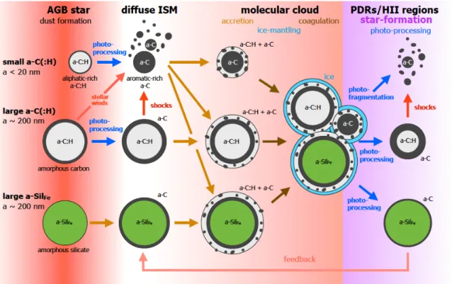
A new dust model has been suggested by Jones et al. (2013) where they use two

dust materials (amorphous carbon, either hydrogenated or not, and amorphous silicates)

and three dust populations (amorphous carbon grains, silicates grains with amorphous

carbon mantle and silicate grains with coagulated amorphous carbon mantle). They show

that their model using the code DustEM and the optEC

(a) optical property data (Jones

2012) explain many FUV and mm dust observables and their inter-correlations. They

also present a schematic view of the dust life circle as shown in Fig. 1.3. The dust grains

travel from the dust shell around AGB stars where they are formed to the diffuse ISM

1.1. Interstellar medium 5

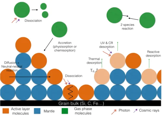
Figure 1.2: Schematic showing the composition of a dust grain and different processes taking place on its surface or within its ice mantle. Image credits: Burke & Brown (2010).

Figure 1.3: Schematic view of the life cycle of interstellar dust. Image credit: Jones et al. (2013).

6 Chapter 1. Introduction Table 1.2: Different regions and their properties.

Regions Diameter (pc) Mean density (cm

)

Protostar 0.01 10

– 10

Dense core 0.1 10

– 10

Clump 1 10

– 10

Molecular cloud 10 10

– 10

Giant molecular cloud 10 – 30 10

– 10

and then due to the core collapse to the dense cores where they accrete, coagulate or re- form. As they transit through the ISM, they are highly altered even destroyed in regions such as H II regions and photon-dominated regions (PDRs) where UV photo-processing is important.

1.2 Star formation

Dense cores, hosts of star formation, result from the condensation and fragmentation of self-gravitating objects referred to as clumps. The clumps are fragmented regions of (giant) molecular clouds too. Cores are not distributed randomly but they are thought to be organized along filamentary structures. They form for instance at the intersection of these gas filaments where matter accumulates through colliding flows (Csengeri et al.

2011). The characteristics of the different objects are found in Tab. 1.2.

Dense cores collapse when they become unstable due to gravitational perturbation such as the passage of Galactic shock wave or supernovae shock wave and once their mass reaches a critical mass, the Jeans mass M

(defined in Eq. 1.1), due to accumulation of material. In the assumption of a homogeneous and spherical cloud, a free-fall collapse happens when the Jeans criteria is fulfilled (see Eq. 1.2, Jeans 1955) i.e., when gravity overcomes the internal pressures (thermal, magnetic) of the cloud. Indeed, at this stage the gas remains cold due to radiative cooling in molecular lines, the gas pressure is thus insignificant.

M

= 1 8

πk

T Gµm

!

1

ρ

, (1.1)

where k

is the Boltzmann constant, T is the temperature of the medium, G is the gravitational constant (G = 6.674×10

m

kg

s

), µ is the mean mass per particle and ρ the density.

E

= 3 2

M

m

k

T ≤ E

= GM

R , (1.2)

where E

is the thermal energy, M the mass of the cloud, m

the hydrogen mass, T the temperature, E

the gravitational potential energy and R the cloud radius.

Collapse does not occur that often as most molecular clouds seem to be gravitationally

stable. These stable clouds are also called sub-critical clouds in opposition to super-critical

clouds which collapse (Shu 1977). This implies that only a small fraction of them form

1.2. Star formation 7

Figure 1.4: Schematic of low mass star formation. Image credit: Luca Carbonaro.

stars. But when it happens, two processes of star formation can be distinguished: low mass star formation (0.1 ≤ M

< 8 M ) and high mass star formation (8 ≤ M

≤ 150 M ).

1.2.1 Theoretical star formation scenario(s)

Low mass star formation

Low mass stars are the main contributors to the total stellar mass of the Galaxy and they

are much more numerous than high mass stars. The low mass star formation scenario

is presented in Fig. 1.4. We briefly summarize it: During the first phase, the pre-stellar

8 Chapter 1. Introduction phase, the core is cold, molecular and does not host a proto-star yet. Then the core enters a contraction phase once gravity becomes stronger than thermal and magnetic pressure. A stellar embryo or proto-star forms at the center of the core and the core becomes optically thick. It concludes the pre-stellar phase and the core enters the proto-stellar phase. The proto-star starts to rotate and an accretion disk appears as the cloud flattens due to gravitational instabilities. The proto-star then evolves through accretion of the envelope material onto the disk and from the disk to the star. This class 0 object is still cold and so it emits in the sub-mm range until it evolves to a class I object and emits in the IR.

During these two stages, class 0 and class I, the proto-star also ejects material without loosing too much mass via bipolar outflows in order to conserve the angular momentum.

Accretion stops once the star reaches its final mass, lower than 8 M , when the radiation pressure is able to overcome gravity. At this point, the proto-star enters the class II phase of the pre-main sequence and is classified as a T-Tauri star. The star emits in the visible/near-IR range while its disk, now called proto-planetary disk is still optically thick and emits in mid and far-IR (FIR). Finally, as the star reaches the class III stage the disk is made of debris and proto-planets.

Massive star formation

Mechanisms to form high mass stars are slightly different as other processes have to occur to counteract the effect of radiation pressure like having a higher accretion rate and a non spherical accretion. Furthermore the low mass star formation scenario does not take into account the fact that massive stars reach the main sequence before accretion is over and it does not explain why massive stars are often found to form in clusters containing low mass and high mass stars. Two main theoretical points of view try to describe high mass star formation: the competitive accretion scenario, e.g. Bonnell, Bate, Clarke, &

Pringle (1997), and the monolithic collapse scenario, e.g. McKee & Tan (2003), also called turbulent core accretion scenario. The first scenario implies that a core gives birth to a star cluster containing a distribution of stars from low to high mass. High mass stars form at the center of this cluster due to the gravitational potential and thus accrete at higher rates. In the same manner binary systems contributes to this differential accretion as they accrete faster due to their potential. Bonnell, Bate, & Zinnecker (1998) also suggest that massive stars could form via collision and merging of lower mass stars assuming a very large stellar density within the cluster. The turbulent core scenario is an extension of low mass star formation scenario and it suggests that the mass of the cores determines the mass of the stars. Thus, massive stars form in massive dense cores unable to fragment contrary to the molecular cloud containing them. The physical processes leading to star formation are self-gravity combined with turbulent motions and magnetic field. In the assumption of an isothermal collapse, high accretion rates as modeled and observed in several regions are difficult to explain. This is not the case for non-thermal pressure support which can induce higher accretion rates needed to form massive stars (McKee

& Tan 2003). The major differences between the competitive accretion scenario and the monolithic collapse scenario are the initial conditions and the physical mechanisms used to produce massive stars. More recently, another scenario stating that the most massive stars form from the global collapse of the molecular cloud has been proposed (Peretto et al.

2007, 2013). This process seems to be in competition with the fragmentation process, also

called the local collapse scenario. In this scenario, two phenomena induce the formation

of the massive star: the first one is the high rate of infalling matter to the center of the

1.2. Star formation 9

Figure 1.5: Schematic of high mass star formation scenario. Image credit: Cormac Purcell.

cloud ( ˙ M > 10

M yr

; Wolfire & Cassinelli 1987, Peretto et al. 2013), the second one is the fragmentation of the cloud into dense cores which migrate to the potential well where they can merge to give even more massive cores.

1.2.2 Massive star formation: From an observational point of view

From an observational point of view, these aforementioned theoretical models of high mass star formation cannot be differentiated easily. Fig. 1.5 presents the evolutionary scenario of massive stars as explained by observers. Within a clumpy (giant) molecular clouds, we find fragments, the cores. At the beginning of their lifetime these cores are cold (T ∼ 10 K) and diffuse (n

∼ 10

– 10

cm

) until they undergo gravitational collapse.

The medium warms up and the density increases. The core reaches the hot molecular core (HMC) phase. The matter is slowly heated up by the proto-star to a temperature of 100 K and above. As the proto-star accretes material from the surrounding envelope, it starts to emit enough UV photons to ionize the neighboring gas and then form an hypercompact (HC) H II region. The ionization front propagates and the HCH II region develops into an ultracompact (UC) H II region and later into a classical H II region and further. Using the adaptive mesh refinement code FLASH

, Peters et al. (2010a) show that HC/UCH II regions do not systematically expand to reach their next evolutionary phase but they can flicker due to variations in the accretion flow. It seems that a rapid increase in the high accretion flow leads to a shrinkage of the H II regions before they expand again. We describe in more detail the HMC and HC/UCH II region phases as well as the PDRs, frontiers between the H II region and the core, in the following subsections.

Hot molecular cores

Once the pre-stellar phase finishes and the warm-up phase occurs, the core enters the HMC phase. HMCs are compact objects (≤ 0.1 pc) which are optically thick with high extinction (A

> 100 mag) and really dense (n

≥ 10

cm

). The embedded proto- star forming at the center of the core heat them up to high temperatures, T ≥ 100 K (Kurtz et al. 2000). HMCs are also transient objects. Their lifetime are around 10

– 10

years (Herbst & van Dishoeck 2009) during which they exhibit a very rich chemistry.

Numerous species, from simple ones to complex organic molecules (COMs), have been

1

http://flash.uchicago.edu/site/

10 Chapter 1. Introduction Table 1.3: Types of HII region and their properties (Kurtz 2005; Hoare et al. 2007).

Regions Size (pc) Density (cm

) Hypercompact ≤ 0.01 ≥ 10

Ultracompact ≤ 0.1 ≥ 10

Compact ≤ 0.5 ≥ 5×10

Classical ∼ 10 ∼ 100

Giant ∼ 100 ∼ 30

Super giant ≥ 100 ∼10

detected (Schilke et al. 2001; Calcutt et al. 2014), principally in the sub-mm regime due to the rotational transitions of COMs. Some well know hot core regions include: OMC–

1 (Blake et al. 1987), Orion–KL (Wright et al. 1996), Sgr B2 (N) (Wilson et al. 1996) as well as G29.96–0.02 (Cesaroni et al. 1994, 1998). Many models have been developed to study their rich chemistry (this will be detailed in Sec. 1.3.3). Furthermore, HMCs are, in contrast to UCH II regions, almost undetectable in the cm-regime as their free-free emission is too weak to be detectable (Hoare et al. 2007). Otherwise, they show a similar spectral energy distribution in the IR/sub-mm frequency range.

Hypercompact/Ultracompact H II regions

HC/UCH II regions trace later stages of massive star formation. HCH II regions might actually coexist with the HMC phase (Beuther et al. 2007). HCH II regions eventually evolve into UCH II regions (Wood & Churchwell 1989; Kurtz 2000; Hoare et al. 2007) but for a period of time the development can be quenched (Walmsley 1995) because of the large mass accretion rates. They can as well fluctuate in sizes and thus going back and forth form a stage to another considering the variations in the accretion flow (Peters et al.

2010a,b). Furthermore, combined with other mechanisms such as outflows the variation of accretion can induce different H II region morphologies.

HCH II regions are approximately ten times smaller than UCH II regions (see Tab. 1.3) and a hundred times denser (Kurtz 2005). Their ionized mass is smaller by one order of magnitude (Ionized mass for HCH II regions ∼ 10

M ; Kurtz 2000) and they are a thousand times brighter. Furthermore, the temperature is extremely high, T

≥ 10

K.

Thus, they have MIR emission originating from the hot dust. In HC/UCH II regions, the central proto-stars are sufficiently evolved to emit UV photons which ionize the surround- ing medium. Photons with energies higher than 13.6 eV are used to ionize molecular hydrogen, thereby, creating an H II region. Photons with lower energies can penetrate the cloud and form an internal PDR ionizing other elements like C-bearing and O-bearing species.

Photon-dominated regions

Photon-dominated regions (PDRs), or photo-dissociation regions, are ubiquitous compo- nents of the ISM. They are produced by the far ultraviolet (FUV) radiation (5.16 eV <

hν < 13.6 eV or in wavelength 912 Å < λ < 2400 Å) coming from the ISM environment

or in the case of internal PDRs by the central protostars of the cores. Even if most of the

FUV photons are absorbed by the dust in PDRs, some of them remain and heat up the

1.3. Chemistry in the ISM 11

Figure 1.6: Schematic representation of a photon-dominated region presenting the different element layers (H

/H/H

, C

/C/CO and O/O

). Image credit: Tielens (2005)

gas. While the photons with energies higher than 13.6 eV dissociate H

and then ionize hydrogen producing the H II region, lower energy photons go through the molecular core and dissociate and ionize other species on their way. The region of the PDR near the ionization front is composed of ions or atoms and deeper zones are composed of atoms and molecules. For instance, as shown in Fig. 1.6, carbon monoxide CO is dissociated to produce C (ionization potential of 11.1 eV) and the carbon is ionized (hν = 11.26 eV) producing C

(also noted C II , the II meaning singly ionized). Oxygen is also ionized into O

(O II ) by photons of energy 13.6 eV.

Internal PDRs are really dense and so very thin because the radiation field cannot penetrate deep into the core (Bruderer et al. 2009a,b; Lee et al. 2015). They are about 200 AU in size, corresponding to a visual extinction A

of 1.6 mag if the density is 10

cm

using the standard Milky-Way values: R

, the ratio of total to selective extinction equal to 3.1 and N

/E(B–V) = 5.8×10

cm

with N

the total column density and E(B–V) the color excess between blue (B) and visual (V) wavelengths.

1.3 Chemistry in the ISM

COMs like methanol (CH

OH), ethanol (C

H

OH) or methyl formate (HCOOCH

) ap- pear to be really abundant in HMCs as mentioned in Sec. 1.2.2. After experimental works showed that formation of COMs is inefficient in the gas phase (e.g., Horn et al. (2004) in the case of methyl formate), an alternative scenario has been proposed as follows: In a cold medium, e.g. during the pre-stellar phase where the temperature is around 10 K, molecules are frozen on the dust grain surface in the densest part of the core (n

≥ 10

cm

). The dust grains formed originally of carbonaceous or silicates compounds build up a mantle mainly made of water and carbon monoxyde. As the medium warms up due to the heating of the proto-star, diffusion of molecules and mostly radicals on the surface can occur around 40 K to form COMs as suggested in Garrod & Herbst (2006).

When the temperature reaches 80 K more COMs are evaporated and released into the

12 Chapter 1. Introduction Table 1.4: Series of gas phase reactions leading to the formation of methyl formate and dimethyl ether (see also Tab. 1 of Balucani et al. (2015)).

OH + CH

OH → CH

O + H

O CH

O + CH

→ CH

OCH

+ hν O + CH

OCH

→ HCOOCH

+ H F + CH

OCH

→ CH

OCH

+ HF Cl + CH

OCH

→ CH

OCH

+ HCl

gas phase and, thus, observable in the hot core phase.

However, this formation scenario of COMs formation is revised as COMs were found in cold dense cores where the temperature is lower than 30 K like in L1689B (Bacmann et al. 2012). A new paradigm has emerged favoring a combined gas-grain chemistry to explain formation of COMs. Balucani et al. (2015) presents new formation routes for methoxy (CH

O), methyl formate and dimethyl ether (CH

OCH

) based on experimental and theoretical works. The conclusions of this paper are presented in Tab. 1.4. They also found this series of gas phase reactions happens after the non-thermal desorption of methanol.

As for chemistry in H II regions, it seems to be mainly influenced by the UV radiation coming from the newly formed massive stars. Most complex molecules are destroyed by the high energy photons at least in the PDRs and their close environment where ionized and neutral atomic species dominate the composition of gas. Deeper in the core where radiation are attenuated by dust more complex molecules are preserved. Chemistry in the ISM depends a lot on the physical conditions and on the quantity of molecules present in the medium. The different chemical processes (see Fig. 1.7) taking place in HMCs, H II regions and PDRs as well as the astrochemical models developed to study them are explained in subsections 1.3.1 and 1.3.2.

1.3.1 Gas phase chemistry

Gas phase chemistry is dominated by two-body reactions, dissociation and ionization reac- tions. A list of gas phase reactions is given in Tab. 1.5. Several kind of two-body reactions are possible which form chemical bonds, destroy them or re-arrange them. In bimolecular reactions, reaction re-arranging the bonds, if A and B are the reactant molecules they react to form an activated complex AB

. This complex decomposes rapidly into two dif- ferent products C and D: A + B → AB

→ C + D. In order for the reaction to start, it requires a certain amount of energy from the local environment, the activation energy, and only collisions with kinetic energy higher than the activation energy lead to a reaction.

These reactions can be exothermic or endothermic. A reaction is endothermic if it receives energy from the environment, i.e. if the energy necessary to break the reactants bonds is higher the energy released during the formation of the products. On the contrary, if the reaction releases energy it is exothermic.

In addition to two-body reactions, there are dissociation and ionization reactions trig-

gered by photons or cosmic-rays. Photo-dissociation/ionization reactions are important