Understanding complex traits by non-linear mixed models

(1)

Understanding complex traits by non-linear mixed models

Inaugural-Dissertation zur

Erlangung des Doktorgrades

der Mathematisch-Naturwissenschaftlichen Fakultät der Universität zu Köln

vorgelegt von

(2)

1. Gutachter: Prof. Dr. Andreas Beyer 2. Gutachter: Prof. Dr. Achim Tresch 3. Gutachter: Dr. Oliver Stegle

Tag der m¨undlichen Pr¨ufung: 8. Oktober 2014

(3)

(4)

(5)

Acknowledgements

First of all, I like to thank my mentor Andreas Beyer, whose group I joined as a PhD student at the BIOTEC in Dresden. During the past years Andreas has not only been a great scientific advisor, but also proven to be a keen manager that always keep my focus on scientific tasks. Under his supervision I enjoyed the freedom to exploit the areas of science that I particularly liked!

Oliver Stegle, who I met as undergraduate student at the Max Planck institute of T¨ubingen, has significantly contributed to this work. He is fa- ther of many ideas that are exploited here. Beyond sharing his exceptional scientific expertise he provided plenty of practical advice. Thanks a lot Oli!

I really enjoyed working with you for the past two years!

I like to thank Achim Tresch who joined our labmeetings with his group. I will miss the (scientific) discussions we had during our weekly lunch breaks.

And thanks a lot for giving me a hand with mathematical problems!

Group members a invaluable for internal reviewing, scientific - and most importantly - social support. So are you! Thanks to Karl Köchert for open minded discussions while having record breaking restaurant bills. Thanks to Julia Harnisch and Susanne Reinhardt for being great in- and out of of- fice mates. All the best to you Sinan Sara¸c and thanks for setting me up at the beginning. Thanks to all members of the fantastic room: Marit Acker- mann, Kalaimathy Singaravelu, Eleni Christodoulou, Mathieu Clément- Ziza, Weronika Sikora-Wohlfeld, Betty Friedrich and Michael Kuhn. And finally, thanks to my lab members from the newly established Cologne group: Li Li, Cédric Debès, Jan Großbach, Mikael Kaminsky, Kay Heit- platz and Marius Garmhausen.

Being at work while feeling among friends never happened to me before.

Thanks a lot to my host group at the EBI: Amelie Baud, Yuanhua Huang, Sung Hee Park and Paolo Casale. I spent a wonderful time with you in Cambridge.

Furthermore, I like to acknowledge people that guided and inspired me during my time as a diploma student at the University of T¨ubingen. I would like to thank my professors for their engagement in turning me into a scientist. In particular I would like to mention professor Hauck, as he is the greatest lecturer I know! My special thanks go to Jacquelyn Shelton for getting me in touch with Oliver Stegle, infecting me with “machine learning” and providing invaluable support during the application for my

(6)

PhD. Thanks a lot Jackie!

I like to thank Aylar Tafazzoli for her constant support and care during the past months when I was primarily occupied writing this thesis.

Finally, I like to thank my parents, grandparents, grandmother and my little brother for being with me throughout my life. It was my family’s constant support that kept me on track and their warm and inspiring environment which enabled me to pursue a scientific career till now.

vi

(7)

Abstract

Population structure and other nuisance factors represent a major challenge for the analysis of genomic data. Recent advances in statistical genetics have lead to a new generation of methods for quantitative trait mapping that also account for spurious correlation as caused by population structure. In particular, linear mixed models (LMMs) gained considerable attention as they enable easy black box-like control for population structure in a wide range of genetic designs and analysis settings.

The aim of this work is to transfer the advantages of LMMs into a random bagging framework in order to simultaneously address a second pressing challenge: the recovery of complex non-linear genetic effects. Existing methods that allow for identifying such relationships like epistasis typically do not provide any robust and interpretable means to control for population structure and other confounding effects.

The method we present here is based on random forests, a bagged variant of the well established decision trees. We show that the proposed method greatly improves over existing methods not only in identifying causal genetic markers but also in the prediction of held out phenotypic data.

Zusammenfassung

Populationsstrukturen sowie andere unerwünschte Faktoren erschweren häufig die Analyse genomischer Daten. Aufgrund von Fortschritten in der statistischen Genetik sind neuere Methoden in der Lage, unerwünschte Korrelationen, die z.B. durch Populationsstrukturen entstehen, zu korri- gieren. Insbesondere haben lineareMixed Models stark an Popularität ge- wonnen. Durch ihre anwenderfreundliche Kontrolle der Populationsstruk- tur sind sie für viele genetische Strukturen und in vielen Studiendesigns anwendbar.

Ziel dieser Arbeit ist es, die Vorteile der linearen Mixed Models mit denen eines Random Bagging Verfahrens zu vereinen, um das Finden komple- xer genetischer Effekte, zu erleichtern. Bestehende Methoden, die solche Signale wie Epistasis erkennen, sind bisher nicht in der Lage, Populati- onsstrukturen und andere St¨orfaktoren zu ber¨ucksichtigen.

Die hier vorgestellte Methode ist eine Erweiterung des Random Forests, eines Random Bagging-Verfahrens welches auf Entscheidungsb¨aumen ba-

(8)

siert. Wie auch bei linearen Mixed Modelskorrigiert es Störfaktoren durch einen Random Effect. Mit Hilfe von simulierten und realen Daten zeigen wir, dass diese neue Methode nicht nur mehr kausale genetische Marker gegenüber bestehenden Ansätzen findet, sondern auch die Vorhersage un- gesehener Phenotypen verbessert.

viii

(9)

Motivation

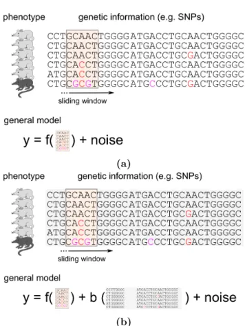
During the past decades biomedical research has received increasing attention as it significantly furthered our understanding of complex medical conditions such as type-II diabetes, Alzheimers- or Crohns disease. In one of its main directions, researchers aim to unveil inherited and environmental contributions to a specific phenotype, as for instance, the state of a disease they are interested in. With steadily increasing amount of genomic data, the application computational tools to guide researchers becomes more and more important. Among these, quantitative trait locus (QTL) mapping methods assess the strength of a link between a genotypic region to quantitative phenotypic condition (trait).

Whereas most QTL mapping methods model phenotypes as a simple linear function of the genotype, it is assumed that for many of the complex diseases multiple genetic factors contribute in a non-linear fashion. In addition, individuals in a sample can be related by means of population structure. Not correcting for such sources of confounding effects leads to an increase in false positive hypotheses and therefore more recent work focuses on correcting for population effects when the underlying genotype to phenotype relationship is linear [28, 30, 34, 50, 66]

On the other hand, numerous alternative approaches have been developed in order to detect non-linear effects like gene-gene epistasis. For example, linear models with interaction terms can be fit using a greedy algorithms [14, 44] or by sampling techniques, e.g. [12]. Also, random bagging techniques [9] have gained considerable attention. In particular, random forests [10] have been shown to accurately capture epistatic effects (e.g. [41, 43, 49]).

All these approaches - including random forests - assume that correlations between genotype and phenotype are genuine and, unlike extensions of linear models, do not explicitly correct for population structure or other confounding effects. Thus, there is a lack of methods that can perform both tasks: correcting for population structure while accounting for epistasis.

(12)

Contents

Outline of this thesis

Following Part I of this thesis, the reader will learn about linear QTL mapping methods and their extensions to correct for population structure as well as decision tree based approaches.

These methodological concepts are required for Part II, where we show how a decision tree based approach can be extended to a simple yet efficient correction for population structure maintaining its ability to map multivariate non-linear associations.

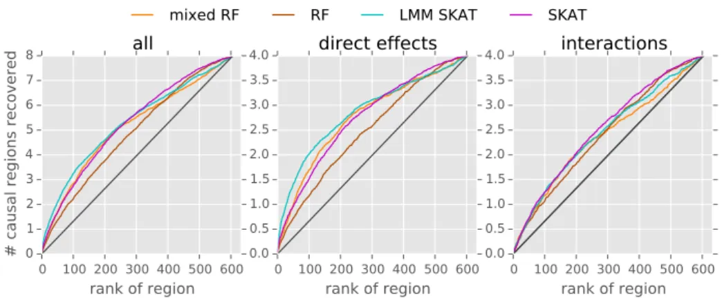
We compare our new approach, termed mixed random forest, to alternative state of the art methods using simulations as well as data obtained from a large scale study in mice [62].

xii

(13)

Part I.

Introduction to genomic

association mapping

(14)

(15)

1 Univariate linear models

Linear models are established tools for QTL mapping. The simplest and probably most commonly used is the so called univariate linear model where a single independent variable like the state of a gene is used to explain a continuous outcome. More elaborate variants are capable of including several features in a linear-additive fashion. We review the univariate model in the following before we discuss several ways to obtain multivariate linear models in Chapter 2.

Assume we are given a continuous phenotypic trait measured for N individuals that is stored within a N-dimensional vector y. Our goal is to explain y as a linear function of genomic information. If we allow for additive noise ψ on our measurements we can write our model as follows

y=β₀+xβ+ψ. (1.1)

Here,xis a real- or integer-valued vector of sizeN that encodes the genetic state for each of individual. Remaining parameters of our model in Equa- tion (1.1) are the weight or slope of our linear functionβ and the intercept with the y-axisβ₀. We shall not concern ourselves with the intercept and thus set β₀ = 0.

For now, β remains the only parameter we want to fit. We optimize this linear model by minimizing the mean squared error between phenotypey and its linear reconstruction xβ w.r.t. β, i.e.

βˆ= arg min

β

1

N ky−xβk² = arg min

β

2 N

1 2

N

X

i=1

(yi−xiβ)²

| {z }

E(β)

. (1.2)

In Section 1.3, we will learn which assumptions are made about the nature of the errorψ when using this so called least squares optimization.

The solution of Equation (1.2) can be found analytically by setting the

(16)

1. Univariate linear models

derivative of the sum of squares error function¹ E(β) w.r.t. β to zero βˆ=

N

X

i=1

x²_i

!⁻¹ _N X

i=1

y_ix_i

!

. (1.3)

We can now evaluate the goodness of the learned model by plugging the optimal solution ˆβ back into Equation (1.2)

E( ˆβ) = 1 2

y−xβˆ

2

, (1.4)

where a low error indicates a good fit. An algorithm for univariate linear association mapping can be established as follows:

1. For each of the given genetic features, optimize the linear model in Equation (1.3) and

2. evaluate the error function (Equation (1.4)) 3. Return the error for each feature

The lower the associated error, the stronger we consider the association between genetic feature and phenotype.

Feature scoring using the error function. Importance measures such as the sum of squares error above only tell about the relative importance of genetic features in a given analysis. This becomes an issue if we intend to compare our results to those of other studies. To obtain more comparable scores, we can evaluate the ratio of the sum of squares errors before and after fitting a model, i.e.

∆ E( ˆβ) = E(0)

E( ˆβ) (1.5)

where

E(0) = 1 2

N

X

i=1

(yi−y)¯ ² (1.6)

and ¯y is the mean of our phenotype across all individuals. This ratio of errors turns out to be proportional to the logarithm of odds (LOD) that is introduced at the end of this chapter.

1Also referred to asresidual sum of squares

4

(17)

1.1. Including covariates

Phenotypes are usually driven by other non-genetic factors like the time at which a measurement was taken, environmental variables such as tem- perature and humidity or even the experimenter herself/himself. We refer to these factors as confounders as there are not of interest to the study.

Careful modelling of such variables is essential to avoid false positive dis- coveries. To illustrate this, suppose there exists a genetic feature which happens to be correlated to a confounder that explains a large fraction of phenotypic variance. If this confounder is not included into our model, the correlated genotypic feature will take its place in explaining phenotypic variance and therefore receive a good score. It is, on the other hand, very unlikely that this particular genetic feature is relevant for the ob- served trait. So what we consider to be genetic driver of our phenotype is probably a false positive.

We can deal with covariates the same way as for genotypic information by including them as linear additive factors into our model, i.e.

y=c1βc1+c2βc2 +· · ·+c_kβc_k+xβ+ψ. (1.7) This turns our univariate- into a multivariate linear model. In the context of (genomic) association mapping, however, it is still considered to be a univariate model as only the importance of a single (genetic) feature xis of interest.

To evaluate the improvement in residual error that can be attributed to x we need to optimize the full model in Equation (1.7) w.r.t. all weights and compute the corresponding error. We do the analogue for the baseline model, which does not include the genomic feature to be tested for association.

Starting with the error functions E0(β_c) = 1

2ky−Cβ_ck² baseline model (1.8) E(β_c, β) = 1

2ky−(Cβ_c+xβ)k² alternative model (1.9) where we introduced the matrix containing the covariates as columns C =

c₁,c₂,· · ·,c_k

and the weight vector β_c =

β_c₁, β_c₂,· · · , β_c_kt

. Af- ter taking the derivative of Equation (1.8) w.r.t. β_c, setting it to zero

(18)

and manipulating the expressions algebraically, we obtain for the baseline model

βˆ_c= C^TC−1

C^Ty. (1.10)

We run the analogue optimization for our alternative model E(β_c, β) and report

∆ E = E₀(βˆ_c)

E(βˆ_c,β)ˆ (1.11)

as score for the association strength of the genetic feature x. Note, that the minimized squared error for the baseline model E₀(βˆ_c) only needs to be computed once.

Fitting the intercept. We can equally regard the intercept β₀ of our model from the beginning (Equation (1.1)) as a N ×1 vector multiplied by the (scalar) weightβ0

y=1β0+xβ+ψ, (1.12)

which allows us to run optimization as before (Equations (1.10) and (1.11)) where the one-valued vector enters as additional covariate.

0.0 0.2 0.4 0.6 0.8 1.0

x (continuous)

−0.5 0.0 0.5 1.0 1.5 2.0 2.5

y

(a)

0.0 0.2 0.4 0.6 0.8 1.0

x (binary)

−0.5 0.0 0.5 1.0 1.5 2.0 2.5

y

β0

β1

(b)

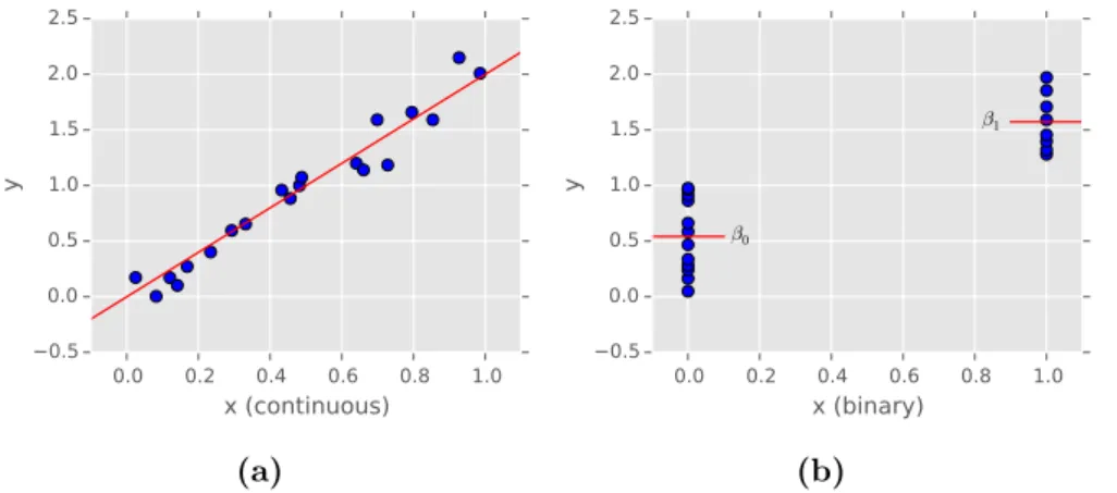
Figure 1.1.: Univariate linear models. (a) 20 individuals are simulated by first sampling uniformly between 0 and 1 in predictor-space x. Corresponding responses in y are then computed as a linear function of xplus a small amount of independent Gaussian noise. (b) the same sample where the predictor values have been “binarized” such that allxi≤0.5 are set to 0 and the remainingxi>0.5 to 1. Red lines indicate the meansβ0 andβ1 as fitted for the two resulting groups of samples.

6

(19)

1.2. Binary predictors

Genetic variants of some stretch of DNA (called ’alleles’) are often distin- guished by measuring single nucleotide polymorphisms (SNPs) in such a region. Assume that Adenin is the most frequent base at a given position in our population and Cytosin being the less common alternative. We say that individuals that contain Adenin are carrier of the major allele, whereas the rest of our population has theminor allele (Cytosin). A common way of encoding is to use “0” to refer to major- and “1” to minor alleles.

For continuous x a linear model can be visualized by a regression line indicating slope and intercept that have been fitted (Figure 1.1(a)). The special case of binary predictors, enables us to take an alternative point of view where the model computes means within two distinct groups: the individuals that containx_i= 0 and the ones that havex_i = 1, respectively.

As shown in Figure 1.1(b), these will turn out to be the intercept β₀ and the weightβ1 from our linear model in Equation (1.12).

Note, that most species have more than a single copy of a chromosome in each cell. Since each copy of a chromosome can harbor a different allele of every marker, in general we have more than two states per marker.

For example, in humans (with two copies per chromosome) we have three possible states: both copies are major, both copies are minor, or one copy is the major and the other the minor allele. However, for task of fitting regression trees, we can still take advantage of this binary perspective by converting a single predictor (that has more than two values) into an equivalent set of binary predictors (see Chapter 4).

1.3. Gaussian interpretation

Now we turn to a probabilistic interpretation of what we referred to as least squares linear model so far. probability distributions. We start by constraining our measurement noise from Equation (1.1) ψ to be Gaus- sian, specifically we have identical and independently (i.i.d.) distributed Gaussian noise with zero mean

ψ∼ N 0, σ²I

. (1.13)

(20)

Including the linear relationship as mean into the noise model, we can regard the phenotype as sample from a Gaussian distribution

y∼ N Cβ_c+xβ, σ²I

. (1.14)

Taking the log transformed log(p(y|x,C,β_c, β, σ²) = N

2 log 1

2πσ²

− 1 σ²

1 2

N

X

i=0

(y_i−(c_iβ_c+x_iβ))²

| {z }

E(βc,β)

.

(1.15) and our goal becomes to maximize this so-called log likelihood w.r.t. the model parametersβ_c,βandσ². This leads to the same optimal solution as by working on the Gaussian directly but the log transformed is preferred for reasons of numerical stability. Furthermore, we notice that the weights β_candβonly depend on the log likelihood only through the negative of the error function −E (β_c, β). In other words, maximizing the log likelihood of a linear model is equivalent to minimizing the least squares in the case of i.i.d. Gaussian noise. We therefore reuse Equation (1.10) to findβˆ_cand βˆ. Putting these optimal weights back into Equation (1.15) and setting the derivative w.r.t. σ² to zero we obtain

ˆ σ²= 1

N

X

i=0

(y_i−(c_iβˆ_c+x_iβ))ˆ ². (1.16) Now we can use our optimal parameters to reevaluate the log likelihood

log(p(y|x,C,βˆ_c,β,ˆ σˆ²) =Nlog 1

2πσˆ²

−N

2 . (1.17) As before we also need to maximize the log likelihood of our baseline model log(p(y|C,βˆ_c,σˆ₀²).

Logarithm of odds. The logarithm of odds (LOD) is defined as LOD = logp(y|x,C,β,ˆ βˆ_c,σˆ²)

p(y|C,βˆ_c,σˆ₀²) = N

2 log(ˆσ₀²)−N

2 log(ˆσ²) (1.18) and can equivalently be computed as difference of the optimized likelihoods for baseline- and alternative model. Associations that have a LOD greater

8

(21)

1.3. Gaussian interpretation than 3 are commonly considered as statistically significant, but in general it is hard to define such a meaningful threshold [3].

P-Values. As alternative to the LOD, we can use the fitted variances of baseline- and alternative model in order to compute the F-Score. This measure can subsequently be used to evaluate the significance of a genetic association by means of a P-Value, see e.g. [3]. P-Values should be handled with care as this approach is very sensitive towards non-normality on the data [7].

(22)

(23)

2 Multivariate linear models

Here we give a brief review on multivariate linear models. Instead of considering a single genetic feature for a given phenotype, multivariate linear models account for multiple effects in a linear-additive fashion, i.e.

y=Cβ_c+x1β1+x2β2+· · ·+xMβM +ψ. (2.1) Once we selected all features to be included, optimization is analog to the linear model with covariates (see Section 1.1).

In most association studies we expect only a small fraction of features to be relevant for the phenotype. A model containing all genotypic information might explain a great proportion of variance, but it is useless if we are to select the subset of features driving phenotypic changes. Therefore, most (if not all) multivariate linear models used today, implement a mechanism to control for the number of features included.

In the following, we present three popular variants of multivariate linear models, a greedy approach called forward selection, its counterpart backward elimination and theLASSO.

2.1. Forward selection and backward elimination

In forward selection we start testing each feature in a univariate linear model for association (using some statistic like the LOD). The feature obtaining the highest score is included as covariate into the (updated) baseline model. This procedure of testing is repeated for the remaining features. Again, the best feature will be included into the baseline model and so on. . . . This way, covariates are added to the model until it cannot be improved by a predefined threshold.

Backward elimination, on the other hand, starts with the model including all covariates. The feature that leads to the least reduction in a predefined score is removed. Covariates are being eliminated as long as reduction in score staysbelow a predefined threshold.

(24)

2. Multivariate linear models

For both of thesestepwise regression methods (see e.g. [24]) the final model contains the set of genetic features considered important.

2.2. The LASSO

The Least Absolute Shrinkage and SelectionOperator (LASSO) [60] is a linear model that, depending on the adjustment of a so called shrinkage parameter, includes a limited number of features.

We derive LASSO extending the linear model’s optimization function by a regularizer that sums over the absolute values of the weights

E(λ,β) = 1 N

1

2ky−Xβk²

| {z }

E(β)

+λ





M

X

j=1

|β_j|





| {z }

regularizer

. (2.2)

To minimize the total error E(λ,β) our aim is to keep the regularizers contribution low. Depending on the choice of λ we encourage weightsβi

that are zero. So, rather than explicitly including or excluding features like in forward selection or backward elimination, LASSO controls the number of active features through their weights.

There is no analytical solution to find the optimum for our objective (Equa- tion (2.2)). Nevertheless, we are dealing with a convex optimization problem and efficient numerical methods are available to obtain good approx- imations. Most LASSO solvers use gradient descent which makes a local quadratic approximation to the optimization function [15].

Bayesian interpretation. We conclude this review of LASSO giving a Bayesian interpretation. By taking the exponent of its negative objective (Equation (2.2))

p(β|y,X)

| {z }

posterior

∝ N y

Xβ, σ²_vI

| {z }

likelihood M

Y

j=1

exp

−1 2λ|β_j|

| {z }

prior

. (2.3)

we find that the regularizer can be seen as Laplace prior over weights β_j whereas our error function E(β) turned into a Gaussian likelihood. As

12

(25)

2.3. Bagging for feature selection in multivariate linear models the marginal p(X,y) is constant, the product of prior and likelihood is proportional to the posterior over the weights. In other words, minimizing LASSO’s objective in Equation (2.2) is equivalent to maximizing the posterior over β in this probabilistic view.

2.3. Bagging for feature selection in multivariate linear models

A problem common to all these methods is that we end up with a set of active predictors while having little information about their relative importance. Note, that considering the LOD or similar statistical measures when including features using forward selection can be misleading. Imagine that the baseline model already includes a covariate which is correlated to a feature we intend to test/include. The feature under consideration is prone to receive a relatively low score, as a significant proportion of phenotypic variance is already accounted for by the other correlated covariate. In the worst case, we may not consider this feature after all. Using the absolute of the weightsβj as importance measure when fitted in a LASSO approach (see Equation (2.2)) is problematic for similar reasons.

There are several methods that address this problem. A conceptually simple way to obtain more robust feature scores uses bagging [9]. That is, we randomly sample N times with replacement from the whole set of individuals. We obtain what is called a bootstrap sample which is used to fit the multivariate linear model of choice. We repeat bootstrapping and fitting several times and record the features selected at each run. The fraction of bootstraps in which a given feature was included in the model is used as importance measure.

Bagging does not come without issues. We need to fit our model several times which can easily exhaust computational resources. In addition, the interpretability of a single linear model is sacrificed for a collection of noisy variants.

For LASSO feature selection, bagging is encouraged by the work of Mein- shausen and B¨uhlmann [40] in which they show that resulting scores are admissible w.r.t. false discovery rates. Bagging has also been successfully applied in combination with forward selection to map complex traits of heterogeneous mouse populations [62].

(26)

(27)

3 Linear mixed models

Linear mixed models are an extension to linear models containing additional summands u1,u2, . . .uK, called random effects

y=Xβ+z₁u₁+z₂u₂+· · ·z_ku_K+ψ, (3.1) were z₁, z₂, . . . z_K weight their relative contributions. Random effects can be regarded as random variables, each following some probability distribution. Here, we will focus on the class of mixed models containing a single Gaussian random effect u, i.e.

y=Xβ+u+ψ (3.2)

where

u∼ N(0,Σ).

Omitting the weight z is not constraining the model as we can simply include zas a factor into the covariance matrix Σ. To keep naming short and simple, we refer to this variant as linear mixed model in the following.

Throughout this work, we use random effects to model those parts of sample variance that are not in the focus of our study. Including known covariates is one way to account for confounding variance (see Chapter 1.1).

However, with large heterogeneous populations, the number of additional factors needed can increase rapidly. Unregularized linear models are then prone to overfit. Random effect modelling, on the other hand, provides a robust way to deal with such complex covariate structures.

3.1. Bayesian motivation of the random effect

We start considering a linear model that just includes our matrix of covariates C

y=Cβ_c+ψ. (3.3)

(28)

3. Linear mixed models

Setting the so called fixed effect Xβ to zero is not compromising the important insights of this Bayesian view, allowing us to update the following derivation for non-zero fixed effects later.

We further assume, that C is a N ×M matrix where M is in the range of N. As mentioned before, joint inference of all covariates using ordinary least squares is prone to result in overfitting. In case of M < N we are guaranteed to run in numerical problems while computing the matrix inversion in Equation (1.10). A common way to address these issues is to introduce a prior distribution over the weights β_c. Here we use an i.i.d.

Gaussian

β_c∼ N 0, σ²_gI

. (3.4)

Multiplying our model forp(y|X,β_c) with the prior, we arrive at the joint distribution of β_cand the observations y

p(y,β_c) =p(y|β_c)p(β_c). (3.5) Direct maximization of this joint distribution w.r.t. β_c would lead to an instance of the so called ridge regression, a method developed in order to more robustly solve ill posed least-squares problems (see for instance [61]).

When modelling nuisance factors, we are not interested in reporting values for the weights β_c (or other types of importance measures). This allows us to take Bayesian modelling one step further marginalizing overβ_c. The resulting model accounts for the whole range of possible configurations of β_c weighted by their prior distribution. Following the usual steps of marginalization would require integrating the joint distribution w.r.t. β_c, i.e.

p(y) = Z

p(y|β_c)p(β_c)dβ_c. (3.6) Our particular case allows a simpler derivation: As both,p(y|β_c) andp(β_c) are Gaussian, it follows that the joint distribution p(y,β_c) is Gaussian as well. Joining the individual quadratic forms

(y−Xβ_c)^TIσ_v⁻²(y−Xβ_c) and β^TIσ⁻²_g β^T

in the exponents to of p(y|β_c) and p(β_c) into an equivalent quadratic form over the concatenated vector [y,β_c]^T we note that the matrix in this quadratic form must be the inverse covariance of the joint distribution.

16

(29)

3.2. Efficient inference in linear mixed models

We have

p(y,β_c) =N(y|Cβ_c, σ_vI)N β_c

0, σ_g²I

=N y

β_c

0 0

,

Iσ_v⁻² Cσ⁻²_v C^Tσ_v⁻² C^TCσ_v⁻²+Iσ_g⁻²

−1!

. (3.7) Applying the rules for Gaussian marginalization (Equation (B.4)) and inversion of partitioned matrices (Equation (B.6)), we find the marginal distribution of y

p(y) =N y

0, σ_g²CC^T+σ_v²I

. (3.8)

Individual samples are now related through the covariance matrixσ_g²CC^T+ σ²_vI. In contrast to our model in Equation (3.5) this marginalized version containsM −1 parameters less.

Let’s get back to our full linear model including a linear fixed effect

y=Xβ+Cβ_c+ψ. (3.9)

Applying the same Gaussian prior and doing the analogue marginalization over β_c, we note that the fixed effect Xβ only enters the mean and not the covariance of the joint distribution Equation (3.7). We find for the updated marginal distribution

p(y|β) =N y

Xβ, σ²_gΣ+σ_v²I

, (3.10)

where we defined Σ:=CC^T. Note, that the fixed effect can be replaced by any function f(X) which is independent of the confounders contained inC.

3.2. Efficient inference in linear mixed models

Linear mixed models can be optimized analytically, but in contrast to the vanilla linear model from before, computational complexity increases drastically. The main reason lies in the inversion of the covariance matrix σ²_gΣ+ σvI that is required to evaluate the derivative of our objective function (log of Equation (3.10)) w.r.t. β. As a result, runtime scales cubic in the number of samples, and if we intend to test M features for

(30)

association, the total computational cost multiplies up to O(M N³). So using the na¨ıve analytical approach will render large scale studies with millions of SNP features infeasible.

More efficient methods joined the scene recently. These reduce runtime by clever algebraic tricks [29, 34, 35, 66] and making weak assumptions about confounding effects [28, 34, 35, 65, 66]. Here, we present in parts the work of Lippert and others [34]. Their proposed FaST LMM utilizes a singular value decomposition (SVD) of Σ in order to reduce the total runtime complexity to O(n³+n²m)¹. The same trick is later applied to the method that is in the focus of this thesis.

We start with the log likelihood of the linear mixed model (Equation (3.10)), this time including all parameters of the conditioning set

LL(β, σ_v², σ²_g) = logp(y|X,β, σ_g², σ²_v) = logN y

Xβ, σ_g²Σ+σ_v²I . (3.11) Our first step is to substitute δ for ^σ_σ^v

g to rewrite Equation (3.11) as LL(β, σ²_g, δ) = log 1

Z −1 2log

1

σ_g²(y−Xβ)^T(Σ+δI)⁻¹(y−Xβ)

. (3.12) Here, Z denotes the Gaussian’s normalizing constant. Second, we replace Σ by a singular value decomposition USU^T, where U is a orthonormal- and S is a diagonal matrix. Utilizing thatUU^T =I, we rearrange Equa- tion (3.12) to

LL(β, σ_v², σ²_g) = log_Z¹ − ¹₂log

1

σ²_g(y−Xβ)^T(USU^T+δUU^T)⁻¹(y−Xβ)

. (3.13) After factoring out U and U^T in the next step, we manipulate the inverse covariance U(S+δI)U^T−1

algebraically to obtainU(S+δI)⁻¹U^T. Plugging this back into Equation (3.13) we have

LL(β, σ²_v, σ_g²) = log_Z¹ +¹₂log

1

σ_g²(U^Ty−U^TXβ)^T(S+δI)⁻¹(U^Ty−U^TXβ) . (3.14) A closer look on this reformulated log-likelihood reveals a quadratic form in U^Ty. In other words, we can alternatively express Equation (3.14) as

1In their work they further show that, when using a low rank approximation of Σ, runtime can even be further reduced.

18

(31)

3.2. Efficient inference in linear mixed models

Gaussian under orthonormal projection by U^T LL(β, σ_g², δ) = logN U^Ty

U^TXβ, σ_g²(S+δI)

= log

N

Y

i=1

N U^Ty

i

U^TX

i:β, σ²_g((Si,i+δ))

. (3.15) The covarianceσ²_g(S+δI) is a diagonal matrix which allows us to factorize our likelihood model. Also note, that the normalization of a Gaussian distribution is invariant w.r.t. orthonormal projection such that Z correctly normalizes this reformulated likelihood. We use this factorized version (Equation (3.15)) for efficient optimization and evaluation in the following.

Optimization w.r.t. β. Setting the derivative of Equation (3.15) with respect toβ to zero we obtain:

βˆ =

" _N X

i=1

1 (Si,i+δ)

U^TXT i:

U^TX

i:

#−1"_N X

i=1

1 (Si,i+δ)

U^TXT i:

U^Ty

i

# . (3.16)

Optimization w.r.t. σ_g². Optimization of Equation (3.15) requires evaluation of the normalization constant Z which we can conveniently write in terms of our diagonal covariance from Equation (3.15)

Z = (2π)^N²

σ²_g(S+δI)

1

2 = (2π)^N²σ²_g

N

X

i=0

(Si,i+δ)

!¹₂

. (3.17) After substituting Z in the log-likelihood by the right hand side of Equa- tion (3.17) we take its derivative w.r.t. σ_g². We find our maxima at

ˆ σ_g²= 1

N

X

i=0

U^Ty

i− U^TX

i:ˆβ 2

(Si,i+δ) , (3.18)

which can be seen as the weighted mean squared error between projected response and (projected) linear prediction.

(32)

Optimization w.r.t. δ. Plugging the expressions for βˆ and ˆσ²_g back in to Equation (3.15) the log-likelihood only depends on δ

LL(δ) = -1 2







N

X

i=1

log (S_i,i+δ) +Nlog 1 N

N

X

i=0

U^Ty

i− U^TX

i:β(δ)ˆ 2

(S_i,i+δ)







−N

2 log(2π)− N 2.

(3.19) Finding the maximum w.r.t. δ is a non-convex optimization problem for which no analytical solution is available. However, once our data {y,X}

has been rotated by U^T, a single evaluation of the log likelihood is linear in sample size N, as compared to O(N³) using Equation (3.12). Thus, we revert to numerical optimization which requires multiple evaluations of the log likelihood for different values of δ. Lippert and others [34] use Brent’s method [11], a simple one-dimensional optimization technique on a fine grid of predefined intervals over δ.

Univariate association tests. Here, we follow in outline the procedure used for the vanilla linear model (see section 1.3). The genetic feature to be tested for association and a one valued vector fitting the intercept are included in the design matrix Xof the alternative model. Our baseline- or null model just includes the intercept. We optimize and evaluate the log likelihood using Equation (3.19) for both models and compute the LOD or P-Value as measure for association strength (see Equation (1.18)).

Lippert and others fit δonce on the null model keeping it fixed for all subsequent association tests. So, in order to assess each genetic feature, they just require a single evaluation of the log likelihood (Equation (3.19)). This trick was first implemented by Kang and others [28] helping to drastically reduce the overall runtime.

3.3. Multivariate linear mixed models

The multivariate linear models presented in Section 2 can be extended to also include random effects. Here, we present the linear mixed model LASSO (LMM LASSO) [50] referring to the work of Segura and others ( [55]) for a treatment on forward selection. Based on the probabilistic interpretation we introduced in Equation (2.3), LASSO is completed to a

20

(33)

3.3. Multivariate linear mixed models random effect model marginalizing over additional covariates as shown for unregularized linear models in Section 3.1

p(β|y,X)∝ N y

Xβ, σ_g²Σ+σ_v²I

M

Y

j=1

exp

−1 2λ|β_j|

. (3.20) Applying the same algebraic tricks introduced in Section 3.2 we can write this posterior as

p(β|y,X)∝ N

˜ y

Xβ, σ˜ _g²IY^M

j=1

exp

−1 2λ|β_j|

(3.21) where ˜y= (S+δI)⁻¹U^Ty and X˜ = (S+δI)⁻¹U^TX,

and we also rescaled the transformed data by (S+δI)⁻¹ to obtain an isotropic Gaussian likelihood. In the space of the transformed data{˜y,X}˜ we arrive at the Bayesian view of the vanilla LASSO Equation (2.3).

Using LASSO solvers on Equation (3.21) requires that δ has been fixed beforehand. A reasonable estimation can be obtained by fitting δ once on the null model (i.e. the model that only includes the intercept) as applied in the univariate case (see Section 3.2).

The shrinkage parameterλcan be found, for instance, using cross-validation.

(34)

(35)

4 Decision tree based approaches

Decision trees are among the oldest machine learning methods and ini- tially developed for use in medical- and military applications [8]. With the introduction of ensemble based approaches such as boosting [19–22] and bagging [9], recently, they regained popularity particularly in the fields of bioinformatics (e.g. [6, 41, 49, 59]) and image analysis (e.g. [5, 47, 56]) Decision trees can either be used for classification or regression [8]. Here, we restrict ourselves to a review ofleast squares regression trees [8] as they are extended by our method that is introduced in Part II. Furthermore, we show that, while being a non-linear method at the global level, building trees can be seen as fitting (multiple) linear models when considering individual operations during learning (splits).

4.1. Least squares regression trees

We follow the notation of [8] and define a least squares regression tree by its set of nodesT ={t₀, . . . , t_n}, wheret₀denotes the root. Note, that indexes of the elements inT are sufficient to specify the exact structure of the tree (see Figure 4.1). Given our response vector of phenotypic observations y inN dimensions and ourN×M matrix of genetic featuresX, let y(t) be the subvector of observations associated to a node t and letN(t) denote the total number of observations at t.

Learning

Learning starts with the tree having only a single nodeT⁽⁰⁾={t₀}to which all observations are associated, i.e. y(t0) = y. When growing the tree at root node t₀, the best splitting point ˆsin the set of possible partitions S is then determined by maximizing the reduction in variance:

ˆ

s= argmax

s∈S

R(t₀)−R(t₁|s)−R(t₂|s), (4.1)

(36)

4. Decision tree based approaches

which leads to daughter nodes t1 andt2. Here we defined for a given node t

R(t) = 1 N(t)

X

i∈t

(y_i−y(t))¯ ²

which corresponds to the within-node variance, and ¯y(t) to the samples’

mean at t.

Viable partitionss∈ S are implied by the candidate featuresx_j, as given by the column vectors ofX. If we assume that - for the sake of simplicity - we are having binary values, there exists at most one possibility to split per feature x_j, i.e. all samples wherex_ij = 1 will be separated from samples having xij = 0. So each feature contributes at most one split to S thus allowing us to operate on the features’ indexes j ∈ {1, . . . , M} directly.

We therefore rewrite equation 4.1 as ˆj= argmax

j∈{1,...,M}

∆R⁰(x_j, t₀) (4.2) where

∆R⁰(x_j, t₀) = R(t₀)−R(t₁|x_ij = 0)−R(t₂|x_ij = 1).

The objective of variance minimization (Equation (4.1)) can equivalently be formulated as maximum likelihood selection of splitting points in a linear model

ˆj= argmax

j∈{1,...,M}

LL(y|βˆ_b,βˆ_j,σˆ_v²,x_j) (4.3) where

LL(y|βˆb,βˆj,σˆ_v²,xj) = logN





 y(t₁)

y(t2)

βˆb

1(t₁) 1(t2)

+ ˆβj

0(t₁) 1(t2)

| {z }

xj

,σˆ²_vI





 .

(4.4) Here,y(t₁) andy(t₂) are reordered versions ofy, such that they correspond to all samples withxij = 0 andxij = 1 respectively. In this representation, βˆb and ˆβj denote sample bias at node t and splitting weight of xj. We summarize this equivalency in

Proposition 1. Let xj ∈ {x₀, . . . ,xM} be a binary predictor andy(t) be

24

(37)

4.1. Least squares regression trees

the measurements associated with node t∈T, then ˆj = argmax

j∈{1,...,M}

∆R⁰(xj, t) = argmax

j∈{1,...,M}

LL(y(t)|β,ˆ σˆ_v²,xj).

A proof of this statement is given in Appendix C.

Splitting proceeds recursively from the subtrees rooted by the daughter nodes t₁ and t₂. Growing of the regression tree is stopped at terminal (or leaf) nodet_T if, either no more splitting is possible (i.e. t_T contains a minimal number of samples) or the scoring function shows no improvement (i.e. ∆R⁰(x_j, t)≈0;∀j).

t0

t₂ t₆ t₅ t₁

t₄ t₃

t0

t₂ t₆ t₅ t₁

t0

t2

t1

t₄ t₃

t₈ t₇

Figure 4.1.: Examples of binary regression using labelling introduced in [8].

Nodes t are indexed starting with zero and subsequently labelled breath-first.

Nodes that do not exist are still counted by the index (as it is the case for the tree in the middle). Using this labelling a node’s index specifies its exact position in the tree.

Features having more than two levels. In cases where we have more than two levels per predictor, we can as well convert this problem into our linear model perspective. The idea is to transform our matrix of features X into an equivalent matrix ˜Xthat leads to same set of splits S.

Suppose that a predictor x has three levels, say 0, 1 and 2¹. In order to partition a given nodetin abinaryregression tree we have two possibilities:

joining all individuals that have x_i < 1 into the first daughter node and the remainder into the second daughter node, or splitting the individuals that havex_i <2 from the rest.

1This encoding is common for organisms that have two copies of a chromosome such as humans. Here we have three possible combinations of alleles for a given marker:

minor-minor, major-minor and major-major.

(38)

Instead of usingxjdirectly we can construct two binary features, where for the first we set all entries havingx_j <1 to 0, the rest being set 1. For the second, all entries in xj smaller than 2 are set to 0 (again, the rest being set to 1). Now, we can apply our splitting objective (Equation (4.1)) and our linear model equivalent (Equation (4.3)) on the alternative features which will lead to the same splits considered than working on xdirectly.

It is straightforward to extend this procedure to features having more than three levels. For each additional level we have to introduce a new binary feature. Consequently, a single feature having k levels can be replaced by k−1 binary features.

Prediction

Using a tree T to predict an outcome (such as disease sate) to given input x? (e.g. the genetic makeup of an individual) is the result of a series of binary decisions. Starting with the root nodet₀, the first decision is based on its feature selected for splitting during learning. Let j be the index of this feature, we proceed to childt1ifxj? = 0 otherwise tot2. We apply this procedure recursively for the subtrees rooted by t₁ or t₂ until a terminal node tT is reached. The prediction (response)y? is given by the average over the training samples associated to tT, i.e. y?= ¯y(tT).

4.2. Random Forests

Random forests (RF) [10] are among the most commonly used ensemble methods. Individual learners - here decision trees - are built on a noisy variant of the training sample (bootstrap). To add further variation to individual trees, splits are performed on a random subset of all available features.

Predictions are obtained by aggregating responses of individual trees. This procedure of bootstrapping, fitting several weak learners and aggregation makes random forest an instance of a bagged² learning method [9].

In our particular case of random forest regression, let{T_b}^B₁ denote such an ensemble ofB trees, whereas each learner is built on a random subsample³ of the data {X,y}. For a test input x?, prediction is defined to be the

2“bagging” is an acronym forbootstrapaggregation

3Both versions, subsampling with and without replacement can be applied

26

(39)

4.2. Random Forests

average response of individual trees, i.e.

f_rf^B(x∗) = 1 B

B

X

b=1

T_b(x∗). (4.5)

Out of bag error

The out of bag error was introduced as an unbiased measure of predictive accuracy for bagged predictors alongside with the initial publication of random forests [10].

As a consequence of subsampling some part of the training data remains unused while building each tree Tb, the so called out of bag sample. Con- versely, to each datum {x_i, y_i} we have a set of trees where {x_i, y_i} is part of the out of bag sample. We can use this subensemble to make a prediction for xi (analog to Equation (4.5)) and take yi to compute the corresponding prediction error.

Repeating this procedure for the rest of the training sample, we take the mean over individual prediction errors to obtain the out of bag error.

Feature scoring

Several feature scoring measures have been proposed for random forests, here we give an overview about the three that are most commonly used.

Breiman [10] suggested the so called permutation importance. That is, after learning the ensemble of trees, values of a specified feature are randomly permuted. The resulting difference in predictive accuracy (estimated with the out of bag error) serves as importance measure for the feature specified.

A simple alternative is theselection frequency (SF)which is the total number a given feature is selected for splitting during learning. Despite being prone to several biases [6, 59] it has proven to be the most sensitive score towards interacting features [41] when compared to alternative measures and methods.

In all our experiments we use the residual sums of squares (RSS) which is the default importance measure of the random forest R package [33].

Briefly, at each node in a tree we add the improvement in variance to the score of the feature chosen for splitting. The sum over all improvements for a given genetic feature is used as final score. This measure behaves similar

(40)

to the selection frequency when it comes to the detection of interacting features [41]. Being on a continuous scale, however, the RSS provides a higher resolution (as compared to selection frequency) which makes this measure is particularly attractive when large data sets with thousands of SNPs and individuals are considered.

28

(41)

Part II.

Mixed random forests

(42)

(43)

5 Mixed model regression trees

Mixed model regression trees extend least squares regression trees by including an additional random effect term (see Figure 5.1). It is the same modelling principle that we applied in Chapter 3 to obtain linear mixed models (LMMs). At every stage of building a mixed model regression tree, variation in the data is modelled by a split according to a selected feature and the random effect. As a consequence of this joint modelling approach, features tend to be selected that lead to splits minimizing those parts of variance which are not captured by the random effect.

In this chapter, we formalize our idea of the mixed model regression tree and explain how computational speed-ups introduced for LMMs (Sec- tion 3.2) can be adapted for our approach, thereby enabling applications to large (genetic) datasets.

5.1. A linear mixed model view

The key innovation of mixed model regression trees is to take advantage of the linear model perspective introduced with least squares regression trees (Equation (4.3)). If we subsequently extend this splitting model by a random effect we obtain following linear mixed model

LL(y|β_b, βj,Σ, σ_g², δ,xj) = logN y

β_b1+βjxj, σ_g²(Σ+δI)

. (5.1) Given feature xj, our objective is to perform a least squares optimization w.r.t. weights β_b (bias),βj (splitting weight) and the random effect variance σ²_g. Like for the LMM and the LMM LASSO in Section 3.2 we estimate δ once on the null model, keeping it fixed during subsequent branching decisions.

In the following, we omit constant parameters on the conditioning set of the likelihood in order to simplify our notation. To assess feature xj as

(44)

5. Mixed model regression trees

ATGCCCTGCAACTGGGGC ATGACCTGCAACTGGGGC ATGACCTGCAACTGGGGC ATGCCCCGCGACTGGGGC ATGACCTGCAACTGGGGC ATGACCTGCAACTGGGGC

ATGCCCTGCAACTGGGGC ATGACCTGCAACTGGGGC ATGCCCCGCGACTGGGGC ATGCCCCGCAACTGGGGC

ATGACCTGCAACTGGGGC ATGACCTGCAACTGGGGC

X1 X2 X3

+

= u

y _X

2

X₃ X₁

f

(

1 2

(

(a)

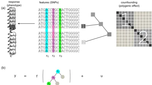
(b) response

(phenotype) features (SNPs) counfounding

(polygenic effect)

Figure 5.1.: Schematic overview of mixed model regression trees. (a)QTL data is considered where individuals are descendants from two different populations as illustrated by the phylogenetic tree. Confounding effects caused by relatedness between individuals are captured by the random effect term with covariance shown on the right. Submatrices corresponding to within relatedness of the two populations are indicated by numbers. Remaining parts of the matrix model cross-relatedness. (b)Response y(coat colour of mice) is modelled by the sum of a (genetic) fixed effect and a random effect. The fixed effect is captured using a decision tree; at the same time, the random effectuwith the covariance derived from the population phylogeny explains confounding by population structure effects. As a result of this joint learning, splits in the regression tree are more likely to occur along informative features that are orthogonal (i.e. not correlated) to confounding effects. In this example the mouse coat colour is a non-linear function of the three polymorphic sites X₁,X₂ andX₃.

candidate for splitting, we evaluate LL(y|βˆb,βˆj,σˆ_g²,xj) = log(N

y

βˆb1+ ˆβjxj,σˆ²_g(Σ+δI)

).

The index of the best predictor can then be found by ˆj= argmax

j∈{1,...,M}

LL(y|βˆ_b,βˆ_j,σˆ²_g,x_j). (5.2) This optimization is equivalent to a (univariate) linear mixed model association test and thus the inference presented in Section 3.2 can be used.

Let ˆxt:=xˆj . As for least squares regression trees (Section 4.1), we apply

32

(45)

5.2. Mixed random forests reordering by combining the samples for which ˆxit= 0 intoy(t1) and leave remaining observations to y(t₂).

In contrast to least squares regression trees, we note that further splitting of the samples in t1 cannot be regarded independently from the samples assigned to t₂ and vice versa. Both branches of the tree remain coupled through the covariance Σ and hence the full dataset needs to be considered in subsequent splits. Tree growing, however, proceeds by recursively selecting further predictors while keeping ˆx_t and the bias in the model.

For node t2 we consider the following mixed model LL

y(t1) y(t₂)

β_b, β_j, σ_g²,x_j

= (5.3)

logN

y(t₁) y(t2)

β^T_bCt2+βj1_[ˆ_x_t_=1](xj), σ_g²(Σ+δI)

where the bias vector and ˆx_t are joined into the matrix Ct2 =

1(t1) 0(t1) 1(t₂) 1(t₂)

and 1_[ˆ_x_t_=1](x_j) denotes the vector having x_ij at all the indices i where ˆ

xit = 1, and 0 otherwise. Alternatively, one can regard 1_[ˆ_x_t_=1](xj) as modelling an interaction between predictors ˆx_t and x_j. Importantly, all the previous weights (which are combined intoβ_b) will be refitted and we find the index of the next splitting feature ˆxt2 by

ˆj= argmax

j∈{1,...,M}

n

LL(y|βˆ_b,βˆj,σˆ²_g,xj) o

. (5.4)

Optimization for node t₁ follows analogously replacing the last summand of the mean in Equation 5.3 with βj1_[ˆ_x₁_=0](xj) and Ct1 by

C_t₁ =

1(t₁) 1(t₁) 1(t₂) 0(t₂)

.

5.2. Mixed random forests

The mixed random forest (mixed RF) is the method in focus of this thesis and obtained by bagging mixed model regression trees. We learn this ensemble analog to random forests creating random subsamples of the