Requirements for Data Quality Metrics

BERND HEINRICH, University of Regensburg DIANA HRISTOVA, University of Regensburg MATHIAS KLIER, University of Ulm

ALEXANDER SCHILLER, University of Regensburg MICHAEL SZUBARTOWICZ, University of Regensburg

Data quality and especially the assessment of data quality have been intensively discussed in research and practice alike. To support an economically oriented management of data quality and decision-making under uncertainty, it is essential to assess the data quality level by means of well-founded metrics. However, if not adequately defined, these metrics can lead to wrong decisions and economic losses. Therefore, based on a decision-oriented framework, we present a set of five requirements for data quality metrics. These require- ments are relevant for a metric that aims to support an economically oriented management of data quality and decision-making under uncertainty. We further demonstrate the applicability and efficacy of these re- quirements by evaluating five data quality metrics for different data quality dimensions. Moreover, we dis- cuss practical implications when applying the presented requirements.

CCS Concepts: • Information systems~Data management systems.

Additional Key Words and Phrases: Data quality, Data quality assessment, Data quality metrics, Require- ments for metrics

1 INTRODUCTION

Due to the rapid technological development, companies increasingly rely on data to support decision-mak- ing and to gain competitive advantage. To make informed and effective decisions, it is crucial to assess and assure the quality of the underlying data. 83% of the respondents of a survey conducted by Experian Infor- mation Solutions [2016] state that poor data quality has actually hurt their business objectives, and 66%

report that poor data quality has had a negative impact on their organization in the last twelve months.

Another report reveals that 84% of the CEOs are concerned about the quality of the data they use for deci- sion-making [KPMG 2016; Forbes Insights 2017]. In addition, Gartner indicates that the average financial impact of poor data quality amounts to $9.7 million per year and organization [Moore 2017]. Overall, it is estimated that poor data quality costs the US economy $3.1 trillion per year [IBM Big Data and Analytics Hub 2016]. In the light of the current proliferation of big data with large amounts of heterogeneous, quickly- changing data from distributed sources being analyzed to support decision-making, assessing and assuring data quality becomes even more relevant [IBM Global Business Services 2012; Buhl et al. 2013; Cai and Zhu 2015; Flood et al. 2016]. Indeed, the three characteristics Volume, Velocity and Variety, often called the three Vs of big data, make the assurance of data quality increasingly challenging (e.g., due to the integration of various data sources or when considering linked data; cf. also Cappiello et al. 2016; Debattista et al. 2016).

Thus, the consequences of wrong decisions are becoming even more costly [SAS Institute 2013; Forbes In- sights 2017]. This has resulted in the addition of a fourth V (=Veracity) reflecting the importance of data quality in the context of big data [Lukoianova and Rubin 2014; Flood et al. 2016; IBM Big Data and Analytics Hub 2016].

Data quality can be defined as “the measure of the agreement between the data views presented by an information system and that same data in the real world” [Orr 1998, p. 67; cf. also Parssian et al. 2004; Hein- rich et al. 2009]. Data quality is a multi-dimensional construct [Redman 1996; Lee et al. 2002; Eppler 2003;

Taleb et al. 2016] comprising different data quality dimensions such as accuracy, completeness, consistency and currency [Wang et al. 1995; Batini and Scannapieco 2016]. Each data quality dimension provides a par-

ticular perspective on the quality of data views. As a result, researchers have developed corresponding met- rics for the quantitative assessment of these dimensions for data views [e.g., Ballou et al. 1998; Hinrichs 2002;

Even and Shankaranarayanan 2007; Heinrich et al. 2007; Fisher et al. 2009; Heinrich et al. 2009; Blake and Mangiameli 2011; Heinrich et al. 2012; Wechsler and Even 2012; Heinrich and Klier 2015; Heinrich and Hris- tova 2016]. Metrics assessing such data quality dimensions for data views and data values stored in IS are in the focus of this paper. In contrast, for instance metrics addressing the quality of data schemes are not directly considered.

Data quality metrics provide measurements for data views with greater (lower) metric values represent- ing a greater (lower) level of data quality and each data quality level being represented by a unique metric value. They are needed for two main reasons. First, the metric values are used to support data-based decision- making under uncertainty. Here, well-founded data quality metrics are required to indicate to what extent decision makers should rely on the underlying data values. Second, the metric values are used to support an economically oriented management of data quality [cf., e.g., Wang 1998; Heinrich et al. 2009]. In this context, data quality improvement measures should be applied if and only if the benefits (due to higher data quality) outweigh the associated costs. To be able to analyze which data quality improvement measures are efficient from an economic perspective, well-founded data quality metrics are needed to assess (the changes in) the data quality level.

While both research and practice have realized the high relevance of well-founded data quality metrics, many data quality metrics still lack an appropriate methodical foundation as they are either developed on an ad hoc basis to solve specific problems [Pipino et al. 2002] or are highly subjective [Cappiello and Comuzzi 2009]. Hinrichs [2002], for example, defines a metric to assess the correctness of a stored data value 𝜔 as 𝐷𝑄(𝜔, 𝜔

) ≔

𝑑(𝜔,𝜔_𝑚)+1

where 𝜔

represents the the corresponding real-world value and 𝑑 a domain- specific distance measure. For instance, as proposed by Hinrichs [2002], let 𝑑(𝜔, 𝜔

) be the Hamming dis- tance between the stored and the correct value (i.e., the number of positions at which the corresponding symbols of two data strings are different). Applying this metric to (𝜔, 𝜔

) = (‘Jefersonn’,‘Jefferson’) and (𝜔, 𝜔

) = (‘Jones’,‘Adams’) to determine the correctness of customers’ surnames in a product campaign yields the following results: 𝐷𝑄(‘Jefersonn’,‘Jefferson’) =

5+1

≈ 16.67% and 𝐷𝑄(‘Jones’,‘Adams’) =

1

4+1

= 20%. If the decision criterion in the product campaign is a metric value of at least 20%, a sales letter is sent to ‘Jones’, which will most probably not reach its destination, whereas no sales letter is sent to ‘Je- fersonn’, which would much more likely reach its destination. To avoid such problems, both researchers and practitioners set out to propose requirements for data quality metrics [e.g., Pipino et al. 2002; Even and Shankaranarayanan 2007; Heinrich et al. 2007; Mosley et al. 2009; Loshin 2010; Hüner 2011]. Most of them, however, did not aim at justifying the requirements based on a decision-oriented framework. As a result, the literature on this topic is fragmented and it is not clear which requirements are indeed relevant to sup- port decision-making. Moreover, as some of the requirements leave room for interpretation, their verifica- tion is difficult and subjective. This results in a research gap which we aim to address by answering the following research question:

Which clearly defined requirements should a data quality metric satisfy to support both decision- making under uncertainty and an economically oriented management of data quality?

To address this research question, we propose a set of five requirements, namely the existence of minimum and maximum metric values (R1), the interval scaling of the metric values (R2), the quality of the configura- tion parameters and the determination of the metric values (R3), the sound aggregation of the metric values (R4), and the economic efficiency of the metric (R5).

We analyze existing literature and justify this set of requirements based on a decision-oriented frame-

work. As a result, our requirements support both decision-making under uncertainty and an economically

oriented management of data quality. Data quality metrics which do not meet them can lead to wrong deci-

sions and/or economic losses (e.g., because the efficiency of the metric’s application is not ensured). Moreo-

ver, the presented requirements facilitate a well-founded assessment of data quality, which is crucial for

supporting data governance initiatives [Weber et al. 2009; Khatri and Brown 2010; Otto 2011; Allen and

Cervo 2015] and an efficient data quality management [cf. also Cappiello and Comuzzi 2009; Fan 2015].

The need for such requirements is further supported by the discussions in other fields of research such as software engineering. For example, Briand et al. [1996] provide a universal set of properties for the sound definition of software measures. The proposed properties can be used by researchers to “validate their new measures” (p. 2) and can be interpreted as necessary requirements for software metrics. In addition, in the context of ISO/IEC standards the SQuaRE series aims to “assist those developing and acquiring software products with the specification and evaluation of quality requirements” [p. V in ISO/IEC 25020 2007; cf. also Azuma 2001]. In particular, ISO/IEC 25020 provides criteria for selecting software quality measures with the same motivation as above.

The remainder of the paper is structured as follows. In the next section, we provide an overview of the related work and identify the research gap. Section 3 comprises the decision-oriented framework for our work. In Section 4, we propose a set of five requirements for data quality metrics which are defined and justified based on this framework. In Section 5, we demonstrate the applicability and efficacy of these re- quirements using five data quality metrics from literature. Section 6 contains a discussion of practical impli- cations. The last section provides conclusions, limitations and directions for future research.

2 RELATED WORK

In this section, we analyze existing works, which propose requirements for data quality metrics. Following the guidelines of standard approaches to prepare the related work [e.g., Webster and Watson 2002; Levy and Ellis 2006], we searched the databases ScienceDirect, ACM Digital Library, EBSCO Host, IEEE Xplore, and the AIS Library as well as the Proceedings of the International Conference on Information Quality (ICIQ) for the following search term and without posing a restriction on the time period: (“data quality” and metric*

and requirement*) or (“data quality” and metric* and standard*) or (“information quality” and metric* and requirement*) or (“information quality” and metric* and standard*). This search led to 136 papers which were manually screened based on title, abstract, and keywords. The remaining 43 papers were analyzed in detail and could be divided into three disjoint categories A, B and C. Category A comprises requirements for data quality metrics and data quality metric values from a methodical perspective. Category B contains require- ments concerning the general data quality assessment process in an organization (e.g., measurement fre- quency). Category C consists of requirements and (practical) recommendations for the concrete organiza- tional integration of data quality metrics (e.g., within business processes). Regarding our research question, we focused on Category A comprising five relevant papers on which we performed an additional forward and backward search, resulting in a total of eight relevant papers discussed in the following.

Pipino et al. [2002] propose the functional forms simple ratio, min or max operation, and weighted average to develop data quality metrics. Simple ratio measures the ratio of the number of desired outcomes (e.g., number of accurate data units) to the total number of outcomes (e.g., total number of data units). Min or max operation can be used to define data quality metrics requiring the aggregation of multiple assessments, for instance on the level of data values, tuples, or relations. Here, the minimum (or maximum) value among the normalized values of the single assessments is calculated. Weighted average is an alternative to the min or max operation and represents the weighted average of the single assessments. The major goal of Pipino et al. [2002] is to present feasible and useful functional forms which can be seen as a first important step to- wards requirements for data quality metrics. They ensure the range [0; 1] for the metric values and address the aggregation of multiple assessments.

Even and Shankaranarayanan [2007] aim at an economically oriented management of data quality. They

propose four consistency principles for data quality metrics. Interpretation consistency states that the metric

values on different data view levels (data values, tuples, relations, and the whole database) must have a

consistent semantic interpretation. Representation consistency requires that the metric values are interpreta-

ble for business users (typically on the range [0; 1] with respect to the utility resulting from the assessed

data). Aggregation consistency states that the assessment of data quality on a higher data view level has to

result from the aggregation of the assessments on the respective lower level. The aggregated result should

take values, which are not higher than the highest or lower than the lowest metric value on the respective

lower level. Impartial-contextual consistency means that data quality metric values should reflect whether the assessment is context-dependent or context-free.

Heinrich et al. [2007; 2009; 2012] analyze how data quality can be assessed by means of metrics in a goal- oriented and economic manner. To evaluate data quality metrics, they define six requirements. Normaliza- tion requires that the metric values fall into a bounded range (e.g., [0; 1]). Interval scale states that the differ- ence between any two metric values can be determined and is meaningful. Interpretability means that the metric values have to be interpretable, while aggregation states that it must be possible to aggregate metric values on different data view levels. Adaptivity requires that it is possible to adapt the metric to the context of a particular application. Feasibility claims that the parameters of a metric have to be determinable and that this determination must not be too cost-intensive. Moreover, this requirement states that it should be possible to calculate the metric values in an automated way.

Mosley et al. [2009] and Loshin [2010] discuss requirements for data quality metrics from a practitioners’

point of view. Both contributions comprise the requirements measurability and business relevance claiming that data quality metrics have to take values in a discrete range and that these values need to be connected to the company’s performance. Loshin [2010] adds that it is important to clearly define the metric’s goal and to provide a value range and an interpretation of the parts of this range (clarity of definition). In addition, Mosley et al. [2009] require acceptability, which implies that a metric is assigned a threshold at which the data quality level meets business expectations. If the metric value is below this threshold, it has to be clear who is accountable and in charge to take improvement actions. The corresponding requirements accounta- bility/stewardship and controllability, however, refer to the integration of a data quality metric within organ- izations (cf. Category C) and are thus not within the focus of this paper. The same holds for the requirements representation and reportability as found in both works and also drill-down capability by Loshin [2010]. Rep- resentation claims that the metric values should be associated with a visual representation, reportability points out that they should provide enough information to be included in aggregated management reports, and drill-down capability states that it should be possible to identify a data quality metric’s impact factors within the organization. Finally, trackability which requires a metric to be repeatedly applicable at several points of time in an organization (cf. Category B) is also beyond the focus of this paper.

Hüner [2011] proposes a method for the specification of business-oriented data quality metrics to support both the identification of business critical data defects and the repeated assessment of data quality. Based on a survey among experts, he specifies 21 requirements for data quality assessment methods (cf. Appendix B).

However, only some of them constitute methodical requirements for data quality metrics and metric values (cf. Category A) and are thus considered further. These are cost/benefit, definition of scale, validity range, comparability, and comprehensibility. The other requirements refer to Category B (e.g., repeatability, defini- tion of measurement frequency, definition of measurement point, definition of measurement procedure) or Cat- egory C (e.g., responsibility, escalation process, use in SLAs) and are not within the focus of this paper.

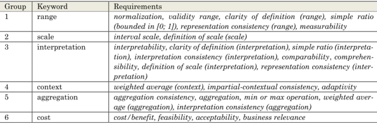
To sum up, prior works provide valuable contributions by stating a number of possible requirements for data quality metrics and their respective values. While some of them overlap, existing literature is still very fragmented. In addition, many requirements are not clearly defined, which makes their application and ver- ification very difficult. To address these issues, we organize the existing requirements in six groups with each group being characterized by a clear, unique characteristic (cf. Table 1). Note that some of the require- ments which leave room for interpretation (cf. brackets in Table 1) are classified in more than one group.

Further, some of these existing requirements (e.g., simple ratio, weighted average) could also be understood

as a way to define a data quality metric. In the following, however, they are considered as requirements for

data quality metrics. For example, simple ratio in Group 1 means that a data quality metric should attain

values in [0; 1].

Table 1. Groups of Requirements

Group Keyword Requirements

1 range

2 scale

3 interpretation

4 context

5 aggregation

age (aggregation), interpretation consistency (aggregation)

6 cost

Group 1 comprises requirements stating that data quality metrics have to take values within a given range.

Simple ratio and representation consistency aim at metric values in the range [0; 1]. Measurability results in a bounded range defined by the lowest and the highest discrete value. Hence, these requirements as well as clarity of definition (with respect to the range), normalization and validity range are assigned to this group.

Group 2 contains requirements regarding the scale of measurement of the metric values. Since definition of scale may not only concern the interpretation of the metric values but also their scale, this requirement is included as well. Group 3 covers requirements claiming an interpretation of the metric values. Here, clarity of definition is interpreted as interpretability. In addition, metric values satisfying the simple ratio require- ment can be interpreted as a percentage, and interpretation consistency requires a consistent semantic inter- pretation of the metric values regardless of the hierarchical level. While comparability, comprehensibility and definition of scale require some kind of interpretation of the metric values (e.g., as a percentage), representa- tion consistency directly implies a clear interpretation with respect to the utility of the data under consider- ation. The requirements in Group 4 state that data quality metrics should be able to consider adequately the particular context of application, for example by means of weights that decrease or increase the influence of contextual characteristics. Group 5 concerns the (consistent) aggregation of the metric values on different data view levels. Min or max operation and weighted average specify how this aggregation has to be per- formed and interpretation consistency requires the same interpretation of the metric values on all data view levels. Finally, Group 6 focusses on the application of a data quality metric from a cost-benefit perspective.

Feasibility is part of this group, because it requires that the costs for determining a metric’s parameters are taken into account and that it should be possible to calculate the metric values in a widely automated way – a fact that results in lower application costs. Business relevance implies that a metric goes along with some benefit for the company, whereas acceptability is part of this group because business expectations are defined considering a cost-benefit perspective.

Table 1 provides an overview of the existing requirements for data quality metrics, which are partly

fragmented and vaguely defined. Prior work does in fact lack a methodical framework and does not aim at

stating and justifying which requirements for data quality metrics support decision-making under uncer-

tainty and an economically oriented management of data quality. To address this research gap, in the next

section we present a decision-oriented framework, enabling us to propose a set of requirements for data

quality metrics in Section 4. In addition to that, the decision-oriented framework helps to clearly and unam-

biguously define the presented requirements as well as to justify them. In this way, it is possible to reason

that a data quality metric should satisfy the presented requirements to support both decision-making under

uncertainty and an economically oriented management of data quality. Finally, this set of clearly defined

requirements combines, concretizes, and enhances the identified groups of existing requirements (cf. Table

1) and thus helps to alleviate the fragmentation within the literature on requirements for data quality met-

rics.

3 DECISION-ORIENTED FRAMEWORK

The decision-oriented framework for our work is based on the following fields: i) decision-making under uncertainty by considering the influence of assessed data quality metric values and ii) economically oriented management of data quality by considering the costs and benefits of applying data quality metrics.

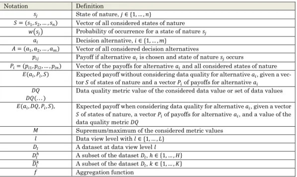
The literature on decision-making under uncertainty (and in particular under risk) uses the well-known concept of decision matrices to represent the situation decision makers are facing [Nitzsch 2006; Laux 2007;

Peterson 2009]. Decision makers can choose among a number of alternatives while the corresponding payoff depends on the state of nature. Each possible state of nature occurs with a certain probability. Hence, in case of a risk-neutral decision maker (if this is not the case, the payoffs need to be determined considering risk adjustments), the one alternative is chosen which results in the highest expected payoff when considering the probability distribution over all possible states of nature. Table 2 illustrates a decision matrix for a simple situation with two alternatives 𝑎

(𝑖 = 1, 2), two possible states of nature 𝑠

(𝑗 = 1, 2), and the respective payoff 𝑝

for each pair (𝑎

, 𝑠

). The probabilities of occurrence of the possible states of nature are repre- sented by 𝑤(𝑠

). To select the alternative with the highest expected payoff, the decision maker has to com- pare the expected payoffs for choosing alternative 𝑎

(i.e., 𝑝

𝑤(𝑠

) + 𝑝

𝑤(𝑠

)) and alternative 𝑎

(i.e., 𝑝

𝑤(𝑠

) + 𝑝

𝑤(𝑠

)). The two-by-two matrix serves for illustration purposes only. Generally, we repre- sent the possible states of nature 𝑠

(𝑗 = 1, … , 𝑛) by the vector 𝑆 = (𝑠

, 𝑠

, … , 𝑠

), the respective probabil- ities of occurrence by 𝑤(𝑠

), the alternatives 𝑎

(𝑖 = 1, … , 𝑚) by the vector 𝐴 = (𝑎

, 𝑎

, … , 𝑎

)

, and the payoffs for alternative 𝑎

by the vector 𝑃

= (𝑝

, 𝑝

, … , 𝑝

). The expected payoff for choosing alternative 𝑎

is denoted by 𝐸(𝑎

, 𝑃

, 𝑆) = ∑

𝑝

𝑤(𝑠

) ; the maximum expected payoff is given by 𝑚𝑎𝑥

𝐸(𝑎

, 𝑃

, 𝑆).

An overview of the notation is provided in Appendix A.

Table 2. Decision Matrix

Requirements for data quality metrics must guarantee that i) the metric values can support decision-making under uncertainty. To address i) it is necessary to examine the influence of data quality and thus of the data quality metric values on the components of the decision matrix (i.e., the probabilities of occurrence, the pay- offs, and the alternatives). In this respect, literature provides useful insights. Heinrich et al. [2012], for exam- ple, propose a metric for the data quality dimension currency [cf. also Heinrich and Klier 2015]. The metric values represent probabilities that the data values under consideration still correspond to their real-world value at the instant of assessing data quality. They apply the metric to determine the probabilities of occur- rence (represented by the metric values) in a decision situation. The influence of data quality on the payoffs is considered, for example, by Ballou et al. [1998], Even and Shankaranarayanan [2007], and Cappiello and Comuzzi [2009]. All of them argue that less than perfect data quality (represented by the data quality metric values) may affect and reduce the payoffs. Other works such as Fisher et al. [2003], Heinrich et al. [2007], and Jiang et al. [2007] examine the influence of data quality on the choice of the alternative.

More precisely, there are several possible ways to express, quantify and integrate the influence of data quality on decision-making. For instance, Even and Shankaranarayanan [2007] consider the effects of data quality on the payoffs for each record of a dataset. They select a subset of attributes which is relevant in the considered application scenario and set the payoffs for a record to zero if the value of at least one relevant attribute is missing. Moreover, having determined the influence of each data quality dimension, there may

1 Note that i) may also be seen as an important means for ii). However, due to the high relevance of i) in the context of data quality metrics, we have decided to distinguish both cases.

2 In case of a continuous decision space, this will be a vector of infinitely many alternatives. If not all alternatives are known, the concept of bounded rationality is applied [Simon 1956, 1969; Jones 1999].

Probability 𝑤(𝑠

Probability 𝑤(𝑠

State 𝑠

State 𝑠

Alternative 𝑎

Payoff 𝑝

Payoff 𝑝

Alternative 𝑎

Payoff 𝑝

Payoff 𝑝

be several ways to weight and aggregate these influences (e.g., by calculating the weighted sum across all data quality dimensions; cf. [Cappiello and Comuzzi 2009]). Therefore, we do not present an explicit formula or method to quantify the influence of data quality on the decision matrix but, instead, specify this impact more generally as follows: Let 𝐷𝑄 represent the data quality metric value and 𝐸(𝑎

, 𝐷𝑄, 𝑃

, 𝑆) the expected payoff for choosing alternative 𝑎

when considering 𝐷𝑄 as well as the payoff vector 𝑃

and the vector of states of nature 𝑆. Let further 𝑚𝑎𝑥

𝐸(𝑎

, 𝐷𝑄, 𝑃

, 𝑆) be the maximum expected payoff when considering data quality. It is obvious and in line with prior works (cf. above) that considering data quality may result in choosing a different optimal alternative as compared to not considering data quality (i.e., 𝑎

= argmax

𝑖

𝐸(𝑎

, 𝐷𝑄, 𝑃

, 𝑆) and 𝑎

= argmax

𝑖

𝐸(𝑎

, 𝑃

, 𝑆) with 𝑎

≠ 𝑎

). Hence, it is useful to consider data quality by means of well-founded metrics in decision-making under uncertainty.

When developing requirements for data quality metrics, it is further necessary to take into account the field of ii) economically oriented management of data quality to avoid inefficient or impractical metrics.

Existing literature has already addressed the question of whether to apply data quality improvement measures from a cost-benefit perspective [Campanella 1999; Feigenbaum 2004; Heinrich et al. 2007; Heinrich et al. 2012]. Indeed, applying data quality improvement measures may increase the data quality level and thus bring benefits. At the same time, the associated costs have to be taken into account and the improve- ment measures should only be applied if the benefits outweigh these costs. In decision-making, the benefits result from being enabled to choose a better alternative (i.e., with an additional expected payoff) due to the improved data quality. The costs include the ones for conducting the improvement measures as well as the ones for assessing data quality by means of data quality metrics. The latter have rarely been considered in the literature, even so they play an important role [Heinrich et al. 2007] and must not be neglected. Indeed, if applying a data quality metric is too resource-intensive, it may not be reasonable to do so from a cost- benefit perspective. Thus, requirements for data quality metrics have to explicitly consider this aspect.

Based on the literature on i) and ii) and the above discussion, Figure 1 presents the decision-oriented framework which is used to justify our requirements [for a similar illustration cf. Heinrich et al. 2007, 2009].

Data quality metrics are applied to data views to assess the data quality level (cf. I-III). The assessed data

quality level (represented by the metric values) influences i) decision-making under uncertainty and in par-

ticular the chosen alternative, and the expected payoff of the decision maker (cf. IV-VI). Thus, the decision

maker may apply improvement measures to increase the data quality level represented by the metric values

(cf. IX). However, applying data quality improvement measures creates costs (cf. VII). This also holds for the

application of the metric including the determination of its parameters (cf. II). Hence, the optimal data qual-

ity level (cf. VIII) has to be determined based on an economical perspective.

IX.

Improvement measures

VII. Costs

VIII. Optimal DQ

VI. Expected payoff II. DQ metric

I. Data values

V. Optimal alternative IV. Alternatives,

states, payoffs III. Assessed DQ

i) Decision matrix ii) Economically oriented

management of DQ

Figure 1. Decision-oriented Framework

4 REQUIREMENTS FOR DATA QUALITY METRICS

In this section, we present a set of five clearly defined requirements for data quality metrics. They combine, concretize, and enhance existing approaches covering the six groups of requirements identified in Section 2.

Moreover, based on the decision-oriented framework we justify that our requirements support both i) deci- sion-making under uncertainty and ii) an economically oriented management of data quality.

4.1 Requirement 1 (R1): Existence of Minimum and Maximum Metric Values

Group 1 states that data quality metrics have to take values within a given range. Most of the requirements in this group (e.g., validity range and clarity of definition) are vaguely defined and thus difficult to verify.

Hence, both the relevance of these requirements and the possible consequences of them not being fulfilled remain unclear (e.g., measurability just claims that the range should be discrete). To address these issues, we propose and justify the following requirement:

Requirement 1 (R1) (Existence of minimum and maximum metric values). The metric values have to be bounded from below and from above and must be able to attain both a minimum (representing perfectly poor data quality) and a maximum (representing perfectly good data quality). In particular, for each real- world value 𝜔

, minimum and maximum value have to be attainable in regard to 𝜔

.

Justification. In a first step, we discuss the following statement (a) which will be used recurrently in the remainder of this justification:

(a) There has to be exactly one metric value representing perfectly good data quality and exactly one

metric value representing perfectly poor data quality.

Re (a): Based on the definition of data quality by Orr [1998] used in this paper, perfectly good data quality implies a perfect agreement between stored data views and the real-world. This is a unique situation and therefore there is exactly one level of perfectly good data quality. In the case of the data quality dimension accuracy, existing metrics use a distance function to measure the difference between the real-world data values and the stored data values. Due to the finite number of possibilities for the stored data values (e.g., a 32 bit integer in Java can represent one of 2

=4,294,967,296 possible numbers; this holds for other data types used for the assessed data value as well), there is always one or more data value(s) for which the distance to the real-world data value is maximal. For this/these data value/s, the data quality level “perfectly poor data”

is reached and cannot become even worse; “even more inaccurate data” cannot be represented. Hence, there is exactly one level of perfectly poor data quality. Summing up and with respect to the discussion of Figure 1, as each data quality level is represented by a metric value and different metric values represent different data quality levels, there has to be exactly one metric value representing perfectly good data quality as well as exactly one metric value representing perfectly poor data quality.

Based on statement (a), we justify (R1). If a data quality metric does not fulfill (R1), this implies that the metric values

(b) are not bounded from below and/or from above and/or (c) do not attain their minimum and/or maximum.

We denote by 𝜔 a stored data value (e.g., a stored customer address) of perfectly good data quality that perfectly represents the corresponding real-world value 𝜔

. Further, we denote the metric value for 𝜔 by 𝐷𝑄(𝜔, 𝜔

).

Re (b): If there is no upper bound for the metric values, another stored data value 𝜔′ can exist which – compared to 𝜔 – results in a higher metric value (i.e., 𝐷𝑄(𝜔′, 𝜔

) > 𝐷𝑄(𝜔, 𝜔

) for the real-world value 𝜔

corresponding to 𝜔 and 𝜔′). As higher metric values represent better data quality, this implies that 𝜔′

is of better data quality than 𝜔. However, 𝜔 was defined to be of perfectly good data quality and only one metric value can represent perfectly good data quality (cf. statement (a)). Hence, the metric values indeed need to be bounded from above. The existence of a lower bound can be justified analogously by using a data value of perfectly poor data quality (e.g., the value ‘NULL’ stored for an unknown customer address which, however, does exist in the real-world).

Re (c): The metric values need to be bounded from below and from above (cf. re (b)). Hence, a supremum 𝑀 (lowest upper bound) exists. If the metric values do not attain a maximum, it follows that 𝐷𝑄(𝜔, 𝜔

) <

𝑀 for a data value 𝜔 of perfectly good data quality. As 𝑀 is the lowest upper bound, there exists another data value 𝜔′′ corresponding to the real-world value 𝜔

with 𝐷𝑄(𝜔, 𝜔

) < 𝐷𝑄(𝜔′′, 𝜔

) < 𝑀 (otherwise, 𝐷𝑄(𝜔, 𝜔

) would be an upper bound and the maximum of the metric values). However, 𝜔 was defined to be of perfectly good data quality. Hence, the metric values indeed have to attain a maximum. The existence of a minimum can be justified analogously by using a data value of perfectly poor data quality.

So far, we discussed the existence of a maximum (representing perfectly good data quality) and a mini- mum (representing perfectly poor data quality) for the metric values with regard to an arbitrary, but fixed real-world value 𝜔

. However, as there is always exactly one metric value representing perfectly good (resp.

poor) data quality (cf. (a)), these maxima and minima coincide across all real-world values. Therefore, the metric values have to be bounded from below and from above and must attain both a minimum and a max- imum (cf. I-III in Figure 1), equal for all real-world values.

When a data quality metric is represented by a mathematical function, (R1) means that this function has to be bounded from below and from above and must attain a minimum and maximum. However, some existing metrics [cf., e.g., Hipp et al. 2001; 2007; Hinrichs 2002; Alpar and Winkelsträter 2014] do not attain a minimum or maximum and may thus lead to a wrong evaluation of decision alternatives (cf. III-VI in Figure 1). In these cases it is, for example, not possible to decide whether the assessed data quality level can or should be increased to allow for better decision-making (cf. VI-IX in Figure 1). As a result, for instance, unnecessary improvement measures for data values of already perfectly good data quality may be performed since the metric values cannot represent the fact that perfectly good data quality has already been reached.

Moreover, when assessing data quality multiple times with a metric which does not satisfy (R1), neither the

comparability nor the validation (e.g., against a benchmark, such as a required completeness level of 90% of

the considered database) of the metric values in different assessments are guaranteed. Moreover, when a specific data quality improvement measure is performed, no benchmark in the sense of a minimum and maximum exists to compare the rankings in the course of time (e.g., consider a user survey regarding the existing data quality level without any information in regard to the scale of values to be entered by the users). This contradicts an economically oriented management of data quality.

4.2 Requirement 2 (R2): Interval-Scaled Metric Values

The requirements in Group 2 focus on the scale of measurement of the metric values. These requirements have not been justified, and some of them do not specify a precise scale (e.g., definition of scale is not defined, but only illustrated by a very wide range of examples). To address this gap, we state and justify the following requirement:

Requirement 2 (R2) (Interval-scaled metric values). The values of a data quality metric have to be interval- scaled

. Based on the classification of scales of measurement [Stevens 1946], this means that differences and intervals can be determined and are meaningful.

Justification. We argue that a metric which does not provide interval-scaled values (cf. I-III in Figure 1) cannot support both the evaluation of decision alternatives and an economically oriented management of data quality in a well-founded way (cf. Section 3). For this, we take into account the decision matrix in Table 2 with the payoff vectors 𝑃

= (𝑝

, 𝑝

) and 𝑃

= (𝑝

, 𝑝

) for the alternatives 𝑎

and 𝑎

and let the expected payoffs for these alternatives be calculated based on the metric values 𝐷𝑄

and 𝐷𝑄

, respec- tively. We consider a situation in which the expected payoffs for choosing alternative 𝑎

and alternative 𝑎

are the same (i.e., 𝐸(𝑎

, 𝐷𝑄

, 𝑃

, 𝑆) = 𝐸(𝑎

, 𝐷𝑄

, 𝑃

, 𝑆)) while 𝑝

> 𝑝

, 𝑝

= 𝑝

, and 𝐷𝑄

< 𝐷𝑄

holds.

Hence, the decision maker faces a situation in which in state 𝑠

choosing alternative 𝑎

goes along with a higher payoff than choosing 𝑎

(𝑝

> 𝑝

), but due to the lower metric value 𝐷𝑄

compared to 𝐷𝑄

, the expected payoff for both alternatives which takes into account the effects of 𝐷𝑄

and 𝐷𝑄

is the same (cf.

III-VI in Figure 1). In this situation, the decision maker is indifferent between the two alternatives

. Thus, the lower payoff for 𝑎

– compared to 𝑎

– is accepted if its estimation is based on data of higher data quality. This means that the decision maker equally evaluates both a change in payoffs from 𝑝

to 𝑝

and a change in data quality metric values from 𝐷𝑄

to 𝐷𝑄

. As both the payoffs and expected payoffs are interval-scaled, the differences between payoffs (resp. expected payoffs) are meaningful and their change can be quantified and evaluated by calculating these differences. To support decision-making under uncer- tainty, this quantified, interval-scaled change in payoffs has to be comparable to a change in data quality.

Hence, it has to be possible to calculate the change between the metric values 𝐷𝑄

and 𝐷𝑄

. When the values provided by a metric are not interval-scaled, there is a missing interpretability of the changes between the metric values compared to the respective existing and meaningful differences in the payoffs which im- pedes the evaluation of decision alternatives. Hence, at most ordinal-scaled data quality metric values cannot support both the evaluation of decision alternatives and an economically oriented management of data qual- ity.

(R2) has a significant practical impact. Indeed, many existing data quality metrics [cf., e.g., Ballou et al.

1998; Hinrichs 2002], which do not provide interval-scaled values, may lead to wrong decisions when eval- uating different decision alternatives (cf. III-VI in Figure 1). Moreover, when evaluating, interpreting and comparing the effects of different data quality improvement measures for an economically oriented man- agement of data quality, interval-scaled metric values are highly relevant. For example, let an ordinal-scaled metric take the values “very good”, “good”, “medium”, “poor” and “very poor”. Then there is no possibility of specifying the meaning of the difference between “very good” and “medium” and a decision maker cannot assess whether it would have the same business value as a difference in payoffs of $500 or $600. In contrast, this difference in payoffs may be equivalent to a difference of 0.2 in metric values for an interval-scaled metric. In particular, it is not enough to state which measure results in the greatest improvement of the data

3 They may also be ratio-scaled, which is a stronger property and includes interval scaling [Stevens 1946].

4 If such a situation does not exist, the decision is trivial: If 𝐸(𝑎₁, 𝐷𝑄₁, 𝑃₁, 𝑆) > 𝐸(𝑎₂, 𝐷𝑄₂, 𝑃₂, 𝑆) holds for 𝑝₁₁> 𝑝₂₁, 𝑝₁₂= 𝑝₂₂ and all possible values for 𝐷𝑄₁ and 𝐷𝑄₂ (i.e., it is not necessarily 𝐷𝑄₁< 𝐷𝑄₂), the decision maker will always choose 𝑎₁ regardless of the metric values. In this case, data quality does not matter, which means that assessing data quality is not necessary at all. The same argumentation applies analogously for 𝐸(𝑎₁, 𝐷𝑄₁, 𝑃₁, 𝑆) < 𝐸(𝑎₂, 𝐷𝑄₂, 𝑃₂, 𝑆) where alternative 𝑎₂ will always be chosen.

quality level based on ordinal-scaled metric values. In the example of an ordinal-scaled metric above, it cannot be determined whether an improvement from “very poor” to “medium” is of the same magnitude as an improvement from “medium” to “very good”. Similarly, it is unclear whether an improvement from “very poor” to “medium” is twice as much as an improvement from “very poor” to “poor”. In contrast, for an interval-scaled metric, an improvement of 0.2 is twice as much as an improvement of 0.1. To ensure the selection of efficient data quality improvement measures, their benefits (i.e., the additional expected payoff) resulting from a clearly specified increase in the data quality level need to be determined precisely and compared to their costs (cf. VI-IX in Figure 1).

The requirements in Group 3 state that the metric values must have an interpretation. However, existing requirements (e.g., comprehensibility, comparability, interpretability, definition of scale, interpretation con- sistency, and clarity of definition) have neither been justified nor do they specify what exactly is meant by interpretation, making the verification of data quality metrics in this regard very difficult. In the following, we argue that we do not need to define a separate requirement for Group 3, because a clear interpretation is already ensured by the combination of (R1) and (R2). Indeed, a metric which meets both (R1) and (R2) is interpretable in terms of the measurement unit one [Bureau International des Poids et Mesures 2006]. To justify this, let 𝑚 be the minimum (representing perfectly poor data quality) and 𝑀 be the maximum (rep- resenting perfectly good data quality) of the metric values (cf. (R1)). Since equal differences result in equi- distant numbers on an interval scale (cf. (R2)), each value 𝐷𝑄 of the metric can be interpreted as the

(𝑀−𝑚)

fraction of the maximum difference (𝑀 − 𝑚). Thus, a data quality metric that meets both (R1) and (R2) is inherently interpretable in terms of the measurement unit one (i.e., as percentage).

A clear interpretation of the metric values is helpful to understand the actual meaning of the data quality level and is thus important in practical applications, such as the communication to business users. This is the case if the metric values are ratio-scaled. Ratio-scaled metric values support statements such as “a metric value of 0.6 is twice as high as a metric value of 0.3”. Ratio-scale can be achieved by a simple transformation of each interval-scaled data quality metric whose minimum 𝑚 of the metric values is transformed to 0 so that each metric value can be interpreted as a fraction with respect to the maximum data quality value.

4.3 Requirement 3 (R3): Quality of the Configuration Parameters and the De- termination of the Metric Values

Group 4 contains requirements stating that it must be possible to adjust a data quality metric to adequately reflect the particular context of application. This, however, addresses only one relevant aspect. There are well-known scientific quality criteria (i.e., objectivity, reliability, and validity) that must be satisfied by data quality metrics but have not been considered in the literature yet. In addition, not only the metric values, but also the configuration parameters of a data quality metric should satisfy these quality criteria to avoid inadequate results (cf. II-III in Figure 1).

To address these drawbacks, we propose and justify the following requirement:

Requirement 3 (R3) (Quality of the configuration parameters and the determination of the metric values). It must be possible to determine the configuration parameters of a data quality metric according to the quality criteria objectivity, reliability, and validity [cf. Allen and Yen 2002; Cozby and Bates 2012; Zikmund et al.

2012]. The same holds for the determination of the metric values.

There exists a large body of literature dealing with the quality criteria objectivity, reliability, and validity of measurements in general [cf., e.g., Litwin 1995; Allen and Yen 2002; Marsden and Wright 2010; Cozby and Bates 2012; Zikmund et al. 2012]. In the following, we first briefly discuss these criteria for the context of data quality metrics. Afterwards, we justify their relevance based on our decision-oriented framework.

Objectivity of both the configuration parameters and the data quality metric values denotes the degree to which the respective parameters and values as well as the procedures for determining them (e.g., SQL que- ries) are independent of external influences (e.g., interviewers). This criterion is especially important for

5 Note that in line with our focus on a methodical perspective on requirements for data quality metrics, we concentrate on methodical criteria. Organizational aspects such as the frequency of applying the metric (defined and idiosyncratic per company) are not discussed.

data quality metrics requiring expert estimations to determine the configuration parameters or the metric values [cf., e.g., Ballou et al. 1998; Hinrichs 2002; Cai and Ziad 2003; Even and Shankaranarayanan 2007;

Hüner et al. 2011; Heinrich and Hristova 2014]. Here, objectivity is violated if the estimations are provided by too few experts or if external influences such as the particular behavior of the interviewers are not min- imized. In general, objectivity becomes an issue if metrics lack a precise specification of (sound) procedures for the determination of the respective parameters and values. In this case, metrics may result in different results if applied multiple times. To avoid highly subjective results and ensure objectivity, the data quality metric and its configuration parameters have to be unambiguously (e.g., formally) defined and determined with objective procedures (e.g., statistical methods; cf., e.g., [Heinrich et al. 2012]).

Reliability of measurement refers to the accuracy with which a parameter is determined. Reliability con- ceptualizes the replicability of the results of the methods used for the determination of the configuration parameters or the metric values. In particular, methods will not be reliable, if expert estimations which change over time or among different groups of experts are involved. Reliability can be analyzed based on the correlation of the results obtained from the different measurements. Thus, data quality metrics which rely on expert estimations [cf., e.g., Ballou et al. 1998; Even and Shankaranarayanan 2007; Hüner et al. 2011;

Heinrich and Hristova 2014] have to define a reliable procedure to determine the configuration parameters and the metric values. Generally, to ensure reliability of the configuration parameters and the metric values, correct database queries or statistical methods may be used. In this case, the result of the respective proce- dure remains the same when being applied multiple times to the same data.

Validity is defined as the degree to which a metric “measures what it purports to measure” [Allen and Yen 2002] or as “the extent to which [a metric] is measuring the theoretical construct of interest” [Marsden and Wright 2010]. Hence, the validity of a method for determining the configuration parameters or the metric values refers to the degree of accuracy with which a proposed method actually measures what it should measure.

Typically, the validity of the determination of a configuration parameter or a metric value is violated if the determination contradicts the aim. There are several examples which illustrate the practical relevance of validity in the context of data quality metrics. The metric for timeliness by Batini and Scanna- pieco [2006, p. 29], for example, involves the configuration parameter 𝐶𝑢𝑟𝑟𝑒𝑛𝑐𝑦 which is intended to rep- resent “how promptly data are updated”. Its mathematical specification 𝐶𝑢𝑟𝑟𝑒𝑛𝑐𝑦 = 𝐴𝑔𝑒 + (𝐷𝑒𝑙𝑖𝑣𝑒𝑟𝑦𝑇𝑖𝑚𝑒 − 𝐼𝑛𝑝𝑢𝑡𝑇𝑖𝑚𝑒), however, seems to contradict this aim. Similarly, Hüner et al. [2011, p. 150]

state that a metric value of zero indicates that “each data object validated contains at least one critical defect”.

However, the mathematical definition of the metric reveals that, to be zero, each data object must actually contain all possible critical defects. Validity can be achieved by consistent definitions, database queries, or statistical estimations constructed to determine the corresponding parameter or value according to its defi- nition. Additionally, restricting the application domain of a metric [cf., e.g., Ballou et al. 1998; Heinrich et al.

2007] also contributes to validity.

Justification. To justify the relevance of (R3) based on the decision-oriented framework, we consider a data quality metric for which objectivity, reliability and/or validity are violated but their values are used to support decision-making under uncertainty (cf. Figure 1). For example, objectivity and/or reliability may be violated due to different expert estimations for the configuration parameters of the metric and validity may be violated due to an inaccurate definition of the metric or its configuration parameters (cf. above). We analyze a decision situation as illustrated by the decision matrix in Table 2. In case objectivity and/or relia- bility are violated, two applications of the data quality metric result in two different data quality levels 𝐷𝑄

and 𝐷𝑄

with 𝐷𝑄

≠ 𝐷𝑄

(e.g., depending on different expert estimations). In case validity is violated, the data quality level 𝐷𝑄

estimated by the metric does not accurately represent the actual data quality level 𝐷𝑄

in the real-world. In either case, consider that 𝐷𝑄

and 𝐷𝑄

result in choosing different alternatives.

To be more precise, this means 𝑎

= argmax

𝑖

𝐸(𝑎

, 𝐷𝑄

, 𝑃

, 𝑆) and 𝑎

= argmax

𝑖

𝐸(𝑎

, 𝐷𝑄

, 𝑃

, 𝑆) with 𝑎

≠ 𝑎

(cf. III-VI in Figure 1). If objectivity and/or reliability are violated, it is not clear to the decision maker whether 𝐷𝑄

, 𝐷𝑄

or none of them correctly reflects the actual data quality level and thus whether 𝑎

or 𝑎

is the accurate decision. Similarly, if validity is violated, then the decision maker will choose 𝑎

6 If validity and reliability are fulfilled for a data quality metric, variations in metric values reflect variations in the level of data quality (i.e., sensitivity is guaranteed; cf., e.g., [Allen and Yen 2002]).

7 In case 𝑎₁= 𝑎₂, data quality does not matter, which means that assessing data quality is not necessary at all (cf. the justification of (R2)).

instead of the accurate choice 𝑎

. Thus, in case objectivity, reliability and/or validity are violated, decision makers will make wrong decisions.

The above justification reveals that data quality metrics which do not fulfill (R3) can lead to wrong deci- sions when evaluating alternatives (cf. III-VI in Figure 1). In addition, such metrics result in serious problems when evaluating data quality improvement measures (cf. VII-IX in Figure 1). Indeed, assessing data quality before and after a data quality improvement measure with a metric not fulfilling (R3) results in inaccurate metric values. This makes it impossible to determine the increase in the data quality level in a well-founded way (e.g., a data quality improvement measure evaluated as effective before its application may not even lead to an increase in the actual data quality level). To support an economically oriented management of data quality, it is thus important to ensure (R3).

4.4 Requirement 4 (R4): Sound Aggregation of the Metric Values

Group 5 addresses the consistent aggregation of the metric values on different data view levels. Again, the requirements in this group are not motivated based on a sound framework. In addition, applying the min or max and the weighted average operations – as proposed by existing works – does not necessarily assure a consistent aggregation. We address these issues by the following requirement:

Requirement 4 (R4) (Sound aggregation of the metric values). A data quality metric has to be applicable to single data values as well as to sets of data values (e.g., tuples, relations, and a whole database). Furthermore, it has to be assured that the aggregation of the resulting metric values is consistent throughout all levels. To be more precise, for data 𝐷

at a data view level 𝑙 + 1 with a disjoint decomposition 𝐷

= 𝐷

∪ 𝐷

∪

… ∪ 𝐷

at data view level 𝑙 (i.e., 𝐷

∩ 𝐷

= ∅ for all 𝑖, 𝑗 ∈ {1, … , 𝐻}, 𝑖 ≠ 𝑗), there has to exist an aggregation function 𝑓: 𝐷𝑄(𝐷

) = 𝑓(𝐷𝑄(𝐷

), … , 𝐷𝑄(𝐷

)) with 𝑓(𝐷𝑄(𝐷

), … , 𝐷𝑄(𝐷

)) = 𝑓(𝐷𝑄(𝐷 ̃

), … , 𝐷𝑄(𝐷 ̃

)) for all disjoint decompositions 𝐷

, 𝐷 ̃

of 𝐷

.

Justification. To justify the relevance of (R4), we argue that a data quality metric needs to (a) be applicable to different data view levels and

(b) provide a consistent aggregation of metric values

in order to support decision-making under uncertainty and an economically efficient management of data quality.

Re (a): Consider a situation (cf. Figure 1) in which data used for decision-making is not restricted to the level of single data values, but also covers sets of data values (e.g., tuples, relations, and the whole database).

This implies that for decision-making under uncertainty and an economically oriented management of data quality, it must be possible to determine data quality at several data view levels.

Re (b): Consider a data quality metric which is defined at both a lower data view level 𝑙 (e.g., relations) and a higher data view level 𝑙 + 1 (e.g., database). In the following, we justify that the metric values must have a consistent aggregation from 𝑙 to 𝑙 + 1. To be more precise, we argue that if an aggregation function 𝑓 for determining the metric value at level 𝑙 + 1 based on the metric values at level 𝑙 does not assure a consistent aggregation, the metric values cannot support decision-making under uncertainty and an eco- nomically oriented management of data quality in a well-founded way (cf. Section 3). In this case, the ag- gregation of the metric values at 𝑙 to the metric value at 𝑙 + 1 does not adequately reflect the characteristics of the underlying datasets at 𝑙 (e.g., size, importance). For our argumentation, we consider a disjoint decom- position of a dataset 𝐷

at 𝑙 + 1 into the subsets 𝐷

(ℎ = 1, … , 𝐻) at 𝑙 (e.g., a database 𝐷

which is decomposed into non-overlapping relations 𝐷

): 𝐷

= 𝐷

∪ 𝐷

∪ … ∪ 𝐷

and 𝐷

∩ 𝐷

= ∅ ∀𝑖 ≠ 𝑗. The metric values for the subsets 𝐷

are denoted by 𝐷𝑄(𝐷

). On this basis, the metric value for 𝐷

can be determined by means of the aggregation function 𝑓: 𝐷𝑄(𝐷

) = 𝑓(𝐷𝑄(𝐷

), … , 𝐷𝑄(𝐷

)). If the aggrega- tion function 𝑓 does not assure a consistent aggregation of the metric values from 𝑙 to 𝑙 + 1, there exists another decomposition 𝐷

= 𝐷 ̃

∪ 𝐷 ̃

∪ … ∪ 𝐷 ̃

of 𝐷

at 𝑙 with 𝐷𝑄

(𝐷

) = 𝑓(𝐷𝑄(𝐷 ̃

), … , 𝐷𝑄(𝐷 ̃

)), 𝐷 ̃

∩ 𝐷 ̃

𝑙

𝑗

= ∅ ∀𝑖 ≠ 𝑗 and 𝐷𝑄

(𝐷

) ≠ 𝐷𝑄(𝐷

). Following this, the resulting metric value for 𝐷

de-

pends on the decomposition of the dataset and can hence be manipulated accordingly (i.e., there are two or

more possible metric values for the same dataset). Thus, we face the same situation as in the justification of

(R3) where it is also not known which metric value actually represents the “real” data quality level of the dataset 𝐷

. It analogously follows that this situation results in wrong decisions (cf. III-VI in Figure 1). To sum up, a data quality metric requires a consistent aggregation of the metric values throughout the different data view levels to support decision-making under uncertainty and an economically oriented management of data quality (cf. Section 3).

When data quality metrics are seen as mathematical functions, (R4) means that these functions for the different data view levels have to be compatible with aggregation. Decision situations usually rely on the data quality of (large) sets of data values. However, many data quality metrics in the literature do not provide (consistent) aggregation rules for different data view levels [cf., e.g., Hipp et al. 2001; Hipp et al. 2007; Li et al. 2012; Alpar and Winkelsträter 2014]. As the above justification reveals, this may lead to wrong decisions when evaluating different decision alternatives (cf. III-VI in Figure 1). In addition, a consistent interpretation of the metric values on all aggregation levels is important to support an economically oriented management of data quality. Otherwise, (repeated) measurements of data quality will provide inconsistent and/or wrong results (e.g., when assessing sets of data values that change their volume over time), making it impossible to precisely determine the benefits of improvement measures and to decide whether they should be applied from a cost-benefit perspective (cf. VI-IX in Figure 1).

4.5 Requirement 5 (R5): Economic Efficiency of the Metric

Finally, Group 6 comprises requirements addressing the cost-benefit perspective when applying data quality metrics

. Existing requirements in this group are not motivated based on a framework. Moreover, for some of them, their definition, specification, and interpretation remain unclear (e.g., business relevance and how to determine the threshold for acceptability), making them difficult to verify. We address these issues by proposing and justifying the following requirement):

Requirement 5 (R5) (Economic efficiency of the metric). The configuration and application of a data quality metric have to be efficient from an economic perspective. In particular, the additional expected payoff from the intended application of a metric has to outweigh the expected costs for determining both the configura- tion parameters and the metric values.

Justification. To justify (R5), we analyze a decision situation as shown in the decision matrix in Table 2.

Let alternative 𝑎

be chosen by a decision maker who does not consider data quality in decision-making (and thus does not apply the metric). Furthermore, let another alternative 𝑎

be chosen if data quality is considered. To be more precise, it holds 𝑎

= argmax

𝑖

𝐸(𝑎

, 𝑃

, 𝑆) and 𝑎

= argmax

𝑖

𝐸(𝑎

, 𝐷𝑄, 𝑃

, 𝑆) with 𝑎

≠ 𝑎

.

In this situation, from a decision-making perspective, considering data quality represents addi- tional information influencing the evaluation of the decision alternatives and their choice. This means that the existing data quality level is an additional information affecting the (ex post) realized payoffs. Thus, the benefit of this additional information is assessed by the difference between the expected payoffs (cf. III-VI in Figure 1) when choosing 𝑎

resp. 𝑎

both under consideration of the additional information, which means, 𝐸(𝑎

, 𝐷𝑄, 𝑃

, 𝑆) − 𝐸(𝑎

, 𝐷𝑄, 𝑃

, 𝑆) [for details cf. Heinrich and Hristova 2016]. Thereby, the application of the data quality metric is economically efficient and therefore justifiable with respect to the decision-ori- ented framework (cf. Figure 1) if and only if the difference between the expected payoffs outweighs the expected costs for applying the data quality metric. Otherwise, the metric contradicts an economically ori- ented management of data quality.

Regarding (R5), especially metrics requiring configuration parameters not directly available to the user have to be analyzed in detail. For example, the metric for correctness by Hinrichs [2002] involves determin- ing real-world values as input, which is usually very resource-intensive and raises the question why a sub- sequent data quality assessment is even necessary (for a detailed discussion cf. Section 5.4). In case of metrics not fulfilling (R5), the determination of the configuration parameters or the procedure for determining the metric values is expected to be too costly compared to the estimated additional expected payoffs (cf. I-IX in Figure 1). In some cases, it may be possible to use automated approximations and estimations (especially for

8 We consider a decision scenario (and the related expected payoffs and costs) in which a data quality metric supports an economically oriented management of data quality from a methodical perspective. We do not focus on organizational aspects such as the conduction of a decision-making process in organizations.

9 In case 𝑎₁= 𝑎₂, data quality does not matter, which means that assessing data quality is not necessary at all (cf. the justification of (R2)).