ATLAS NOTE ATLAS-CONF-2012-040

ATLAS-CONF-2012-040 29March2012

ATLAS NOTE

ATLAS-CONF-2012-040

March 29, 2012

Measurement of the Mistag Rate of b-tagging algorithms with 5 fb⁻¹ of Data Collected by the ATLAS Detector

The ATLAS collaboration

Abstract

The mistag rates of several b-tagging algorithms have been measured with two comple- mentary methods using data from the ATLAS detector. The measurements use inclusive jet samples selected from 5 fb⁻¹ of data collected in 2011. The first method uses the invariant mass spectrum of tracks associated with reconstructed secondary vertices to separate light and heavy-flavour jets, and the other is based on the rate at which secondary vertices with negative decay length, or tracks with negative impact parameter, are present in the data.

The measurements of the mistag rate are provided in the form of jet-pTandηdependent scale factors that correct the b-tagging performance in simulation to that observed in data.

Good consistency is observed between the results of the two methods. The uncertainties range from less than 10% for the loosest operating points to more than 100% for the tightest operating points.

1 Introduction

The identification of jets originating from b-quarks is an important part of the LHC physics program.

In precision measurements in the top quark sector as well as in the search for the Higgs boson and new phenomena, the suppression of background processes that contain predominantly light-flavour jets using b-tagging is advantageous. It might also become critical to achieve an understanding of the flavour structure of any new physics (e.g. Supersymmetry) revealed at the LHC.

In order for b-tagging to be used in physics analyses several quantities have to be measured: the efficiency with which a jet originating from a b-quark is tagged by a b-tagging algorithm, referred to as the b-tag efficiency, as well as the probabilities of mistakenly b-tagging a jet originating from a c-quark or a light-flavour parton (u-, d-, s-quark or gluon), referred to as the c-tag efficiency and mistag rate respectively. This note describes the mistag rate measurements.

The b-tagging algorithms calibrated in this note are SV0, IP3D+SV1, JetFitterCombNN, JetFitter- CombNNc and MV1. More details about SV0 can be found in [1], while the IP3D+SV1 and JetFitter- CombNN algorithms are described in [2]. The JetFitterCombNNc algorithm is identical to JetFitter- CombNN with the exception that the neural network is trained to reject c-jets rather than light-flavour jets. The MV1 algorithm is a neural network-based algorithm that uses the output weights of IP3D, SV1 and JetFitterCombNN as inputs.

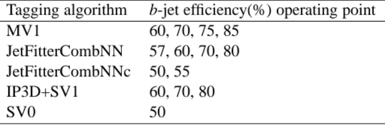
For each b-tagging algorithm a set of operating points is defined, based on the inclusive b-tag effi- ciency in a simulated sample of t ¯t events. The operating points for which calibration results are reported in this note are listed in Table 1.

Tagging algorithm b-jet efficiency(%) operating point

MV1 60, 70, 75, 85

JetFitterCombNN 57, 60, 70, 80 JetFitterCombNNc 50, 55

IP3D+SV1 60, 70, 80

SV0 50

Table 1: The tagging algorithms and operating points for which calibration results are presented in this note.

The mistag rate is measured in data using two methods, both based on an inclusive sample of jets.

The two methods, referred to as the negative tag and sv0mass methods, are briefly described in the following. More details can be found in [3].

The calibration results are presented as scale factors defined as the ratio of the mistag rates in data and simulation:

κ_ε^data/sim_l =ε_l^data

ε_l^sim (1)

whereε_l^sim is the fraction of light-flavour jets which are tagged in simulated events, with the jet flavour defined by matching to generator level partons, while ε_l^data is the measured value of the mistag rate in data.

2 Event selection and data samples

The data sample used in the analyses corresponds to approximately 5 fb⁻¹ of 7 TeV proton-proton

negative tag sv0mass

|η| |η|

p_T(GeV) [0,1.2] [1.2,2.5] [0,1.2] [1.2,2.5]

20-30 635661 530445 518691 421421 30-60 2080302 1606412 1500920 1162410 60-140 3891436 2554054 2415426 1684880 140-300 8296143 4038642 5210343 2713028

300-450 4796003 1684644 - -

450-750 885325 183795 - -

Table 2: The number of jets per jet pTandηbin selected in data by the negative tag (left) sv0mass (right) analyses.

measurement was collected using a logical OR of single jet triggers which select events with at least one jet with transverse energy above a given threshold at the highest trigger level. The thresholds, expressed in GeV, are: 10 , 15 , 20, 30, 40, 55, 75, 100, 135, 180, 240. These triggers have been heavily prescaled to a constant bandwidth of about 0.5 Hz each and reach an efficiency of 99% for events having the leading jet with an offline energy higher than the corresponding trigger thresholds by a factor ranging between 1.5 and 2.

The key objects for b-tagging are the reconstructed primary vertex, the calorimeter jets and tracks reconstructed in the inner detector, consisting of silicon pixels, silicon strips and drift tubes. The track- selection criteria depend on the b-tagging algorithm, and are detailed in [1, 2]. Jets are reconstructed from topological clusters [4] of energy in the calorimeter using the anti-kt algorithm with a distance parameter of 0.4 [5–7]. The jet reconstruction is done at the electromagnetic scale and then a scale factor is applied in order to obtain the jet energy at the hadronic scale. The measurement of the jet energy, the current status of the jet energy scale determination and the specific cuts used to reject jets of bad quality are described in [8]. The tracks are associated with the calorimeter jets with a spatial matching in∆R(jet,track)[9].

Since a well-reconstructed primary vertex is important in b-tagging analyses, the number of tracks associated to the primary vertex is required to be at least two. The jets are required to have p_T>20 GeV and|η|<2.5. The sv0mass analysis only uses, for each jet-p_Tbin, jets for which the trigger that fired the event is fully efficient in that bin, while the negative tag analysis uses the two leading jets in each event and requires them to be in a back-to-back configuration∆ϕ>2.

The number of jets per jet p_T and jet η bin selected by the negative tag and sv0mass analyses are reported in Table 2. The sv0mass analysis limits the jet pT range to 300 GeV because of the reduced sensitivity of the secondary vertex mass at high jet p_T.

The analyses make use of the inclusive QCD jet sample for which the simulation has been carried out in seven slices of ˆp_⊥, the momentum of the hard scatter process perpendicular to the beam line [10].

About 2.8 million events have been simulated per ˆp_⊥ slice. The sample is generated with PYTHIA 6 [10], utilizing the ATLAS AUET2B LO** PYTHIA tune [11]. To simulate the detector response, the generated events are processed through a GEANT4 [12] simulation of the ATLAS detector, and then reconstructed and analyzed in the same way as the data [13]. The simulated geometry corresponds to a perfectly aligned detector and the majority of the disabled pixel modules and front-end chips seen in data were masked in the simulation. The simulation configuration used for the production of the samples used in this note is the same as the one used for the generation of simulation samples for physics analyses ensuring coherence between calibration measurements and their use in physics analyses.

To bring the simulation into agreement with data for distributions where discrepancies are known to

be present, corrections have been applied to the simulated QCD jet sample in the mistag rate analyses.

The p_T spectrum of jets in the simulated QCD jet sample is softer than in data as the prescaling of the low threshold triggers is not activated in simulation. Since the b-tag efficiency and mistag rate depend strongly on the jet kinematics, the jet pT and η distributions in simulation have been simultaneously reweighted to agree with those observed in data. A reweighting for the average number of interactions per bunch crossing (µ) has also been performed to ensure good agreement between data and simulation in the number of reconstructed primary vertices per event.

The labeling of the jet flavour in simulation is done by spatially matching the jet with generator level partons: if a b-quark is found within∆R=p

(∆η²+∆φ²)<0.3 of the jet direction, the jet is labeled as a b-jet. If no b-quark is found the procedure is repeated for c-quarks and τ-leptons. A jet for which no such association could be made is labeled as a light-flavour jet.

3 Measuring the Mistag Rate

The mistag rate is defined as the fraction of jets originating from light flavour which are tagged by a b-tagging algorithm. Since the mistag rate depends on the kinematics of the jet under consideration, the measurement is performed in bins of jet pTand jetη.

The measurement of the mistag rate has been performed by using two independent methods: the negative tag method and the sv0mass method. Both methods are described in detail in [3]. In the following a short description of the methods, including the most relevant updates, is presented.

3.1 The Negative Tag Method

Light-flavour jets are mistakenly tagged as b-jets mainly because of the finite resolution of the inner detector and the presence of tracks stemming from displaced vertices from long-lived particles or material interactions. Prompt tracks which are seemingly displaced due to the finite resolution of the tracker will as often appear to originate from a point behind as in front of the primary vertex with respect to the jet axis. In other words, the lifetime-signed impact parameter distribution of these tracks, as well as the signed decay length of vertices reconstructed from these tracks, are expected to be symmetric.

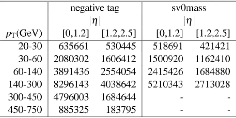
The inclusive tag rate obtained by reversing the impact parameter significance sign of tracks for impact parameter based tagging algorithms, or reversing the decay length significance sign of secondary vertices for secondary vertex based tagging algorithms, is therefore expected to be a good approximation of the mistag rate due to resolution effects. For the SV0 tagger, which is a basic secondary vertex based algorithm where the tag weight W is the signed decay length significance of the reconstructed secondary vertex, a jet is considered negatively tagged if it contains a secondary vertex with decay length signifi- cance W<w rather than decay length significance W>w, where w is reference weight cut for a particular efficiency. For advanced tagging algorithms, based on likelihood ratios or neural networks, the negative tag rate is instead computed in a more complex way, defining a negative version of the tagging algorithm which internally reverses the impact parameter and the decay length selections. For such algorithms, a jet is consider negatively tagged if it has a negative tag weight W_neg>w rather than W_pos>w. Figure 1 shows the tag weight distribution of the SV0 algorithm, as well as the negative and positive tag weight distributions for the JetFitterCombNN algorithm. For the SV0 algorithm, the tag weight distribution is almost symmetric about zero for light-flavour jets, and the negative side of the tag weight distribution is dominated by light-flavour jets. For the JetFitterCombNN algorithm, the standard and negative tag weight distributions for light-flavour jets are similar except for very low and high tag weight values, while the tag weight distributions for b- and c-jets differ substantially. For reference the weight cut value w for the JetFitterCombNN tagger, corresponding to a b-jet efficiency of 60%, is 1.8.

SV0 weight -15 -10 -5 0 5 10 15 20 25

Events

103

104

105

b-jets c-jets light-flavour jets

ATLAS Preliminary

JetFitterCombNN weight

-4 -3 -2 -1 0 1 2 3 4

Normalized distribution

10-5

10-4

10-3

10-2

10-1

1 light-flavour jets

light-flavour jets, negative tag b-jets, negative tag c-jets, negative tag

ATLAS Preliminary

Figure 1: The SV0 tag weight distributions for b-, c- and light flavour jets in simulation (left) and the JetFitterCombNN negative tag weight normalized distribution in simulation, for b-, c-, and light flavour jets separately, as well as the JetFitterCombNN tag weight normalized distribution for light flavour jets in simulation (right). The cut value on the JetFitterCombNN weight corresponding to 60% b-jet efficiency is 1.8.

The mistag rateεl is determined by the negative tag rate of the inclusive jet sample,ε_inc^neg corrected by two factors:

• the negative tag rate for b- and c-jets differs from the negative tag rate for light-flavour jets. b- and c-jets are positively tagged mainly because of the measurable lifetimes of b- and c-hadron decays, shifting the decay length significance distributions towards larger values. However, effects like the finite jet direction resolution can flip the sign of the discriminating variable, increasing significantly the negative tag rate for b- and c-jets. The correction factor k_hf=ε_l^neg/ε_inc^negis defined to account for this effect. Because of the effects described above and the relatively small fractions of b- and c-jets in the inclusive sample, k_hfis typically smaller than, but close to, unity.

• A symmetric decay length or impact parameter significance distribution for light-flavour jets is only expected for fake secondary vertices arising e.g. from track reconstruction resolution effects.

However, a significant fraction of reconstructed secondary vertices have their origin in charged particle tracks stemming from long-lived particles (K_s⁰,Λ⁰etc.) or material interactions (hadronic interactions and photon conversions). These vertices will show up mainly at positive decay length significances and thus cause an asymmetry for the positive versus negative tag rate for light-flavour jets. The correction factor kll=εl/ε_l^negis defined to account for this effect. Because of the sources in light-flavour jets showing positive decay length, k_ll is larger than unity. In particular k_ll ranges, depending on jet p_T and on the operating point, between 2 and 3 for SV0, between 1 and 4 for IP3D+SV1, between 1 and 33 for JetFitterCombNN, and between 1 and 13 for MV1.

The measured negative tag rate valueε_inc^neg is hence converted to the mistag rateεl using the above correction factors khfand kll:εl=ε_inc^negkhfkll. Both correction factors are derived from simulation.

3.2 The sv0mass Method

The sv0mass method uses the invariant mass of charged particles associated to an inclusively recon- structed secondary vertex to separate light-flavour, c- and b-jets. Templates of the sv0mass are derived from simulation, separately for the pre-tagged and tagged samples, in bins ofη and p_T for the different flavours.

The fit of the sv0mass templates to the pre-tagged secondary vertex mass distribution in data deter- mines the number of b-, c- and light-flavour jets in the pre-tagged sample (Nb, Ncand Nl) while a similar fit to the subsample selected by applying the tagging requirement gives the corresponding number of tagged jets (N_b^tag, Nc^tagand N_l^tag). The mistag rate for light-flavour jets is then given by:

εl=N_l^tag Nl

. (2)

In the previous version of the sv0mass analysis [3] the secondary vertex mass templates were fitted to data only in the tagged sample, while the number of light-flavour jets in the pre-tagged sample was deduced using the relation

Nl=Ndata−Nb−Nc=Ndata−N_b^tag εb

−Nc^tag

εc

. (3)

The b-jet and c-jet tagging efficiencies were determined in simulation and corrected by the scale factors measured by the p^rel_T method [3]. This approach induces a correlation between the b-tag efficiency mea- surements and the mistag rate measurements. This correlation is considerably reduced by the approach presented in this note.

Examples of sv0mass template fits to data in the pre-tagged sample as well as a sample of jets tagged by the MV1 tagging algorithm at 70% efficiency, for jets with jet pT in the interval [30,60] GeV and jet

|η|<1.2, are shown in Fig. 2. In the cases where no secondary vertex is reconstructed, the sv0mass of a

jet is set to a default value of -1.

SV0 Mass [GeV]

-1 0 1 2 3 4 5 6

Entries per 0.5GeV

10 102

103

104

105

106

data b-jets c-jets

light-flavour jets ATLAS Preliminary

SV0 Mass [GeV]

-1 0 1 2 3 4 5 6

Entries per 0.5GeV

0 2000 4000 6000 8000 10000 12000 14000 16000 18000

data b-jets c-jets

light-flavour jets ATLAS Preliminary

Figure 2: Examples of sv0mass template fits to the pre-tagged sample of jets with jet p_T in the interval [30,60] GeV and jet |η|<1.2 (left) and to the corresponding jet sample tagged by the MV1 tagging algorithm at 70% efficiency (right).

4 Systematic Uncertainties

The sv0mass and negative tag analyses have common contributions to the systematic uncertainties com- ing from the imperfect knowledge of the jet energy scale and resolution and from the modeling of the detector activity arising from additional proton-proton collisions in the same bunch crossing as the col- lision of interest, so called pileup interactions. Other systematic uncertainties are different for the two methods. Nevertheless some of them might be partially correlated, for instance changing the fraction of long-lived particles and fake tracks, which are one source of the systematic uncertainty for the negative tag method, will also affect the sv0mass templates.

The systematic uncertainties on the mistag rate scale factorκ_ε^data/sim_l of the MV1 tagging algorithm at 70% efficiency are shown in Tables 3 and 4 for the negative tag method and Tables 5 and 6 for the sv0mass method, for jets with|η| ∈[0,1.2]and|η| ∈[1.2,2.5]respectively. The systematic uncertainties have a positive (negative) sign if the difference between the shift in the scale factor when applying a positive and a negative variation of the underlying parameter is positive (negative). In the negative tag analysis, in cases where the statistics in simulation are not sufficient to evaluate with sufficient precision the effect of a given systematic variation, the systematic uncertainty has been evaluated by merging two adjacent jet p_Tbins.

Source Jet p_T[GeV]

[20,30] [30,60] [60,140] [140,300] [300,450] [450,750]

Simulation statistics 4 2 1 1 1 1

Data taking period dependence -13 3 3 6 -3 4

Jet vertex fraction -6 1 <1 <1 <1 <1

Jet energy scale <1 <1 -1 <1 <1 <1

Jet energy resolution <1 -1 2 <1 <1 <1

Trigger bias 17 13 12 12 18 21

k_hf: b fraction 1 1 2 3 3 3

khf: c fraction 1 3 5 6 6 5

k_hf: b-tag efficiency 2 3 5 7 7 5

k_hf: c-tag efficiency 4 6 9 11 10 9

kll: long lived particles -5 -9 -11 -3 7 15

k_ll: fake tracks -1 -1 <1 <1 -2 -2

k_ll: material interactions 1 <1 1 <1 <1 <1

Track multiplicity 1 1 3 8 11 15

Impact parameters smearing -3 -3 6 6 -4 -4

total systematic 24 18 22 23 27 33

statistical 1 1 <1 <1 <1 1

Table 3: Relative systematic and statistical uncertainties, in %, on the mistag rate scale factorκ_ε^data/sim_l from the negative tag method for the MV1 tagging algorithm at 70% efficiency for jets with|η| ∈[0,1.2].

4.1 Simulation statistics

The fit to the sv0mass distribution is performed neglecting the fluctuations of the sv0mass templates due to limited simulation statistics. The effect on the measurement is evaluated by randomly varying the content of each bin of the templates according to its statistical uncertainty, and repeating the template fit

Source Jet p_T[GeV]

[20,30] [30,60] [60,140] [140,300] [300,450] [450,750]

Simulation statistics 8 3 3 3 3 6

Data taking period dependence -10 6 -2 7 -10 -1

Jet vertex fraction 2 <1 -1 <1 1 -1

Jet energy scale -4 -1 -1 <1 <1 -2

Jet energy resolution -9 -3 -1 13 7 36

Trigger bias 10 13 19 7 4 -3

k_hf: b fraction 1 <1 1 2 1 2

khf: c fraction 1 1 3 4 4 5

khf: b-tag efficiency 2 1 3 5 4 3

k_hf: c-tag efficiency 3 4 6 7 7 7

kll: long lived particles 4 -13 -8 7 <1 -17

kll: fake tracks 19 19 11 11 3 3

k_ll: material interactions 1 <1 <1 <1 <1 <1

Track multiplicity <1 2 3 11 13 15

Impact parameters smearing -11 -11 -10 -10 -22 -22

total systematic 29 30 27 27 30 49

statistical 2 1 1 1 1 2

Table 4: Relative systematic and statistical uncertainties, in %, on the mistag rate scale factorκε^data/siml

from the negative tag method for the MV1 tagging algorithm at 70% efficiency for jets with |η| ∈ [1.2,2.5].

Source Jet p_T[GeV]

[20,30] [30,60] [60,140] [140,300]

Simulation statistics 2 7 5 6

Data taking period dependence -10 14 8 7

µ reweighting <1 -3 -2 -2

Jet vertex fraction 16 4 1 2

Simulation efficiency model -10 -9 -9 -13

Jet energy scale -3 -1 1 -1

Jet energy resolution 3 <1 -1 -1

Template shape 2 7 6 6

SV0 efficiency 26 30 31 21

Pre-tagged light jets yield -3 -5 -5 -6

total systematic 33 36 34 28

statistical 4 3 2 1

Table 5: Relative systematic and statistical uncertainties, in %, on the mistag rate scale factorκ_ε^data/sim_l from the sv0mass method for the MV1 tagging algorithm at 70% efficiency for jets with|η| ∈[0,1.2].

Source Jet p_T[GeV]

[20,30] [30,60] [60,140] [140,300]

Simulation statistics 4 11 6 8

Data taking period dependence -12 19 3 4

µ reweighting -1 -9 -5 8

Jet vertex fraction 25 7 2 3

Simulation efficiency model -4 -9 -10 -10

Jet energy scale 5 -1 <1 1

Jet energy resolution -5 4 3 5

Template shape 3 7 4 3

Sv0 efficiency 35 43 32 20

Pre-tagged light jets yield -4 -6 -6 -10

total systematic 46 51 36 28

statistical 6 4 2 1

Table 6: Relative systematic and statistical uncertainties, in %, on the mistag rate scale factorκ_ε^data/sim_l from the sv0mass method for the MV1 tagging algorithm at 70% efficiency for jets with|η| ∈[1.2,2.5].

to data. The RMS of the scale factor distribution from these pseudo-experiments is taken as a systematic uncertainty in the sv0mass analysis.

In the negative tag analysis the limited simulation statistics affect the precision of the kll and khf

correction factors and this uncertainty is propagated to the final result as a systematic uncertainty.

4.2 Data taking period dependence

In order to study the dependence of the results on the amount of pileup, data and simulation samples have been split in three subsequent data taking periods with increasing amount of pileup. The variation of the resulting scale factor between the first and last data taking period is taken as a systematic uncertainty in both analyses.

To avoid fluctuations in the sv0mass templates due to reduced simulation statistics, the templates determined on the entire simulated sample have been used, reweighted to the jet pT andη spectrum in each data taking period.

4.3 Jet vertex fraction

Jets originating from pileup interactions can be rejected by requiring that the tracks associated to the jet are compatible with originating from the selected primary vertex. The fraction of compatible tracks is referred to as the jet vertex fraction or JVF. Many physics analyses in ATLAS are considering only jets with a large JVF (typically above 0.75). The data-to-simulation scale factors derived only from jets with a JVF above 0.75 is compared to those obtained without a cut on the JVF, and the difference is treated as a systematic uncertainty.

4.4 Jet energy scale

A jet energy scale in simulation which is different from that in data would bias the p_Tdistribution of the simulated events. The systematic uncertainty originating from the jet energy scale is obtained by scaling the pTof each jet in the simulation up and down by one standard deviation, according to the uncertainty of the jet energy scale [8].

4.5 Jet energy resolution

The jet energy resolution in simulation is smeared to agree with that in data. The smearing parameters have been varied within their uncertainties, and the effect on the final result is treated as a systematic uncertainty. In the negative tag analysis the application of this procedure to simulated events, for some of the low efficiency operating point, leaves some of high jet-p_T bins empty. The systematics in these specific cases has been evaluated by merging the three highest jet-pTbins.

4.6 µ reweighting

In both the negative tag and sv0mass analyses, the simulated sample has been reweighted based on the average number of interactions per bunch-crossing (µ) to agree with the corresponding distribution in data. In the negative tag analysis the simulation is reweighted to the µ distribution in data after the analysis trigger selection while in the sv0mass analysis, the reweighting has been done using the µ distribution in data for events selected by a single trigger representing, on average, the pileup behaviour of the bulk of the data.

Since theµ-distribution for the various triggers used in the analyses vary substantially, the conserva- tive estimate based on reweighting to the trigger with the smallest and largest amount of pileup is taken as a systematic uncertainty in the sv0mass analysis.

4.7 Trigger bias

The negative tag analysis uses the two leading jets in each event and requires them to be in a back-to-back configuration,∆ϕ>2. As a consequence generally only one of the two jets is in the jet p_Tregion where the single jet trigger used to select the events is fully efficient. In order to take into account possible biases coming from differences in data and simulation in the trigger turn-on region and in the isolation of the leading and sub-leading jet, the measurement has been repeated using only the jet with sub-leading

p_T. The variation in the mistag rate is taken as systematic uncertainty.

The trigger bias systematic uncertainty is one of the dominant in the negative tag analysis. The main reason is that the number of associated tracks in the sub-leading jets is not well modelled by simulation.

4.8 k_hfuncertainty

In the negative tag analysis, the systematic uncertainty due to heavy flavour fractions in the negatively tagged sample is estimated by varying the b- and c-fractions by 10% and 30%, respectively. These uncertainties are taken as the difference between the heavy flavour fractions measured in data and the simulation values using sv0mass fits (as described in [3]). The systematic uncertainty due to the negative tag rate of heavy flavour jets is estimated by varying the negative b- and c-tag rates by 20% and 40%, respectively. These values are conservatively deduced by doubling the systematic uncertainties on the corresponding positive tagging rates estimated by the p^rel_T method [3].

4.9 k_ll uncertainty

The systematic uncertainty due to the limited knowledge of k_ll in the negative tag analysis is evaluated by varying in simulation the different sources contributing to this factor. The dominant contributions considered here include decays of long-lived particles, fake tracks, and interactions in the material of the tracker.

The variations have been performed by substituting the kll determined in the inclusive jet sample with the one obtained from a sub-sample of jets in which a given contribution has been removed. This

of the jets (approximately 8%) do not contain tracks from material interactions, the above procedure cannot be used to deduce the effect on k_llfrom material interactions due to a lack of simulation statistics.

Instead the number of jets containing tracks from material interactions has been varied by 10% (removing events from the appropriate categories).

The variation arising from each of the three components have been summed in quadrature and taken as systematic uncertainties.

4.10 Track multiplicity

The simulation does not properly reproduce the multiplicity of tracks associated with jets observed in data. This could be due to imperfect modeling of fragmentation differences in the relative fraction of quark and gluon jets in the light-flavour sample or differences in the track reconstruction efficiency be- tween data and simulation. A higher track multiplicity implies a larger probability of accidentally tagging a light-flavour jet as a b-jet for purely combinatorial reasons. The systematic uncertainty in the negative tag analysis due to the track multiplicity is estimated by reweighting the jet sample according to the ratio of distributions of the number of tracks associated to jets in data and simulation. The track multiplicity systematic uncertainty is affecting the higher jet pTbins more because the discrepancy between data and simulation is larger in that region.

4.11 Impact parameter smearing

The b-tagging performance is very sensitive to the resolution of the fitted track parameters and the proper estimation of the errors, especially in light-flavour jets where a large fraction of the b-tagged jets originate from prompt tracks which appear to be displaced.

The systematic uncertainty in the negative tag analysis arising from possible differences between the track impact parameter resolution for data and simulation is estimated by evaluating the correction factors k_hf and k_ll on a simulated sample where additional impact parameter smearing was introduced. The smearing parameters used in this analysis are based on measurements of the impact parameter resolution and its uncertainty in data with the method described in [14].

4.12 Simulation efficiency model

The seven simulated samples corresponding to different slices of the transverse momentum of the hard scatter process have been optimally used in the different jet-p_T bins in order to minimize the statistical fluctuations while keeping a good representation of the p_T distribution in each bin. Variations of the mistag rate in simulation due to changes in this default configuration have been considered to estimate systematic uncertainties.

4.13 Pre-tagged light-flavour yield

To evaluate the systematic effects on the yield estimate of pre-tagged light jets in the sv0mass analysis, an independent estimate is obtained using the method adopted in [3]. In this alternative approach, the flavour composition of the pre-tagged sample is inferred from that of the tagged sample by making use of the b- and c-tag efficiencies [15]. The scale factor variation due to this alternative computation of the number of light jets in the pre-tagged sample is taken as a systematic uncertainty in the sv0mass analysis.

4.14 Template shape

Since the sv0mass template shapes are determined from simulation, systematic uncertainties can arise from discrepancies in the sv0mass distribution between data and simulation. The template shapes have

been varied linearly about the median bin using the slope of the ratio of the sv0mass distributions in data and simulation, based on a study done with 2010 data [3]. A conservative safety factor of two has been applied to the slope to account for possible differences between the 2011 and 2010 data. The effect on the scale factor is taken as a systematic uncertainty in the sv0mass analysis.

4.15 SV0 efficiency

When the secondary vertex mass is not reconstructed the sv0mass variable takes a default value of -1, making the template shape dependent on the vertex reconstruction efficiency and its proper modeling in simulation. To evaluate the effect of a possible difference between the vertex reconstruction efficiency in data and simulation, the vertex component of the heavy flavour (light flavour) templates is scaled by 15%

(30%) but restricting the variation of the default bin (corresponding to events for which the secondary vertex has not been reconstructed) to no more than 10% (20%). The motivation for these variations relies on the observation that the b-tag efficiency scale factor, measured with the p^rel_T method, for the SV0 tagging algorithm at an operating point corresponding to 50% b-tag efficiency, does not differ from unity by more than 15% [15]. The fit was repeated with the modified templates and the effect on the final result is considered as a systematic uncertainty in the sv0mass analysis.

5 Results

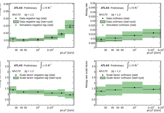
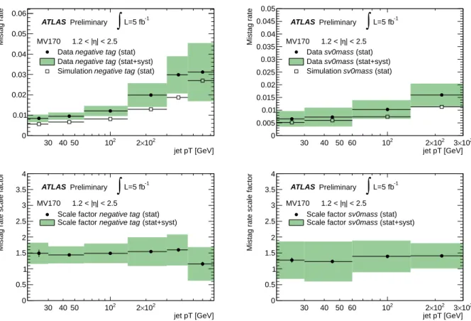
The measured mistag rates in data, the mistag rates in simulation and the resulting data-to-simulation scale factors for the MV1 tagging algorithm at 70% efficiency are shown in Figures 3 and 4 for the negative tag and sv0mass methods, for two different regions of the jet pseudorapidity. Results for other tagging algorithms and operating points can be found in Tables 7 and 8.

The agreement between the two methods is satisfactory, and the systematic uncertainties are of simi- lar size. For this particular tagging algorithm and operating point the efficiency in data tends to be higher than in simulation, leading to data-to-simulation scale factors which are above unity.

6 Conclusions

Two methods, based on a sample of inclusive jets, have been used to measure the mistag rate of several algorithms with 5 fb⁻¹of data from the ATLAS detector. The results are expressed in terms of scale fac- tors, correcting the mistag rate in simulated events to those measured in data. The scale factors measured with the two methods are consistent with each other within uncertainties. The uncertainties on the scale factors depend strongly on the operating point and range from less than 10% for the loosest operating points to more than 100% for the tightest operating points. Moreover, the uncertainties depend on jet p_T and η. For the MV1 tagging algorithm at 70% efficiency they range from 18% in the intermediate pT

range for central jets to as much as 49% in the high p_Tregion for forward jets.

References

[1] ATLAS Collaboration, Performance of the ATLAS Secondary Vertex b-tagging Algorithm in 7 TeV Collision Data, ATLAS-CONF-2010-042, May, 2010.

[2] ATLAS Collaboration, Commissioning of high performance b-tagging algorithms with the ATLAS detector, ATLAS-CONF-2011-102, July, 2011.

jet pT [GeV]

30 40 50 10² 2×10²

Mistag rate

0 0.01 0.02 0.03 0.04 0.05 0.06

MV170 |η| < 1.2

(stat) negative tag Data

(stat+syst) negative tag

Data

(stat) negative tag Simulation

ATLAS Preliminary

∫

jet pT [GeV]

30 40 50 60 10² 2×10² 3×10²

Mistag rate

0 0.005 0.01 0.015 0.02 0.025 0.03 0.035 0.04 0.045 0.05

MV170 |η| < 1.2 (stat) sv0mass Data

(stat+syst) sv0mass

Data

(stat) sv0mass Simulation

ATLAS Preliminary

∫

jet pT [GeV]

30 40 50 10² 2×10²

Mistag rate scale factor

0 0.5 1 1.5 2 2.5 3 3.5 4

MV170 |η| < 1.2

(stat) negative tag Scale factor

(stat+syst) negative tag

Scale factor

ATLAS Preliminary

∫

jet pT [GeV]

30 40 50 60 10² 2×10² 3×10²

Mistag rate scale factor

0 0.5 1 1.5 2 2.5 3 3.5 4

MV170 |η| < 1.2

(stat) sv0mass Scale factor

(stat+syst) sv0mass

Scale factor

ATLAS Preliminary

∫

Figure 3: The mistag rate in data and simulation (top) and the data-to-simulation scale factor (bottom) for MV1 tagging algorithm at 70% efficiency obtained with the negative tag method (left) and the sv0mass method (right) for jets with|η|<1.2

[3] ATLAS Collaboration, Calibrating the b-Tag Efficiency and Mistag Rate in 35 pb⁻¹of Data with the ATLAS Detector, ATLAS-CONF-2011-089, June, 2011.

[4] ATLAS Collaboration, The ATLAS Experiment at the CERN Large Hadron Collider, JINST 3 (2008) S08003.

[5] M. Cacciari, G. P. Salam, and G. Soyez, The anti-k(t) jet clustering algorithm, JHEP 04 (2008) 063.

[6] M. Cacciari and G. P. Salam, Dispelling the N**3 myth for the k(t) jet-finder, Phys. Lett. B641 (2006) 057.

[7] M. Cacciari, G. P. Salam, and G. Soyez. http://fastjet.fr/.

[8] ATLAS Collaboration, Jet energy measurement with the ATLAS detector in proton- proton collisions at sqrt(s) = 7 TeV,arXiv:1112.6426 [hep-ex].

[9] ATLAS Collaboration, Expected performance of the ATLAS experiment: Detector, Trigger and Physics, Volume 1, CERN-OPEN-2008-020, December, 2008.

[10] T. Sjostrand, S. Mrenna, and P. Z. Skands, PYTHIA 6.4 Physics and Manual, JHEP 05 (2006) 026.

[11] ATLAS Collaboration, Further tunes of PYTHIA6 and Pythia 8, ATL-PHYS-PUB-2011-014, November, 2011.

jet pT [GeV]

30 40 50 10² 2×10²

Mistag rate

0 0.01 0.02 0.03 0.04 0.05 0.06

MV170 1.2 < |η| < 2.5 (stat) negative tag Data

(stat+syst) negative tag

Data

(stat) negative tag Simulation

ATLAS Preliminary

∫

jet pT [GeV]

30 40 50 60 10² 2×10² 3×10²

Mistag rate

0 0.005 0.01 0.015 0.02 0.025 0.03 0.035 0.04 0.045 0.05

MV170 1.2 < |η| < 2.5 (stat) sv0mass Data

(stat+syst) sv0mass

Data

(stat) sv0mass Simulation

ATLAS Preliminary

∫

jet pT [GeV]

30 40 50 10² 2×10²

Mistag rate scale factor

0 0.5 1 1.5 2 2.5 3 3.5 4

MV170 1.2 < |η| < 2.5

(stat) negative tag Scale factor

(stat+syst) negative tag

Scale factor

ATLAS Preliminary

∫

jet pT [GeV]

30 40 50 60 10² 2×10² 3×10²

Mistag rate scale factor

0 0.5 1 1.5 2 2.5 3 3.5 4

MV170 1.2 < |η| < 2.5 (stat) sv0mass Scale factor

(stat+syst) sv0mass

Scale factor

ATLAS Preliminary

∫

Figure 4: The mistag rate in data and simulation (top) and the data-to-simulation scale factor (bottom) for MV1 tagging algorithm at 70% efficiency obtained with the negative tag method (left) and the sv0mass method (right) for jets with 1.2<|η|<2.5

[12] GEANT4 Collaboration, S. Agostinelli et al., GEANT4: A simulation toolkit, Nucl. Instrum. Meth.

A506 (2003) 250–303.

[13] ATLAS Collaboration, The ATLAS Simulation Infrastructure, Eur. Phys. J. C70 (2010) 823–874, arXiv:1005.4568 [physics.ins-det].

[14] ATLAS Collaboration, Tracking Studies for b-tagging with 7 TeV Collision Data with the ATLAS Detector, ATLAS-CONF-2010-070, July, 2010.

[15] ATLAS Collaboration, Measurement of the b-tag Efficiency in a Sample of Jets Containing Muons with 5 fb⁻¹of Data from the ATLAS Detector, ATLAS-CONF-2012-021, February, 2012.

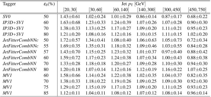
Tagger εb(%) Jet p_T [GeV]

[20,30] [30,60] [60,140] [140,300] [300,450] [450,750]

SV0 50 1.43±0.61 1.02±0.24 1.01±0.29 0.86±0.14 0.87±0.17 0.68±0.22

IP3D+SV1 60 1.63±0.68 1.23±0.33 1.24±0.39 1.07±0.26 1.07±0.28 0.90±0.30 IP3D+SV1 70 1.38±0.33 1.13±0.25 1.17±0.27 1.09±0.20 1.11±0.21 0.95±0.23 IP3D+SV1 80 1.21±0.20 1.08±0.16 1.12±0.16 1.10±0.15 1.11±0.15 1.02±0.20 JetFitterCombNNc 50 1.72±0.57 1.34±0.41 1.08±0.40 1.06±0.63 1.05±0.73 0.72±0.34 JetFitterCombNNc 55 1.69±0.35 1.35±0.31 1.18±0.32 1.09±0.46 1.03±0.55 0.84±0.28 JetFitterCombNN 57 1.43±0.70 1.15±0.25 1.23±0.32 1.01±0.37 0.97±0.40 0.88±0.42 JetFitterCombNN 60 1.59±0.72 1.17±0.23 1.24±0.38 1.07±0.34 1.00±0.43 0.88±0.38 JetFitterCombNN 70 1.33±0.28 1.18±0.18 1.20±0.27 1.09±0.28 1.10±0.30 0.94±0.30 JetFitterCombNN 80 1.20±0.18 1.07±0.14 1.12±0.16 1.12±0.19 1.16±0.22 1.07±0.25

MV1 60 1.58±0.66 1.14±0.24 1.22±0.38 1.02±0.35 1.04±0.37 0.82±0.35

MV1 70 1.38±0.33 1.18±0.22 1.19±0.26 1.09±0.25 1.09±0.30 0.92±0.30

MV1 75 1.29±0.27 1.15±0.19 1.17±0.23 1.09±0.20 1.11±0.25 0.93±0.23

MV1 85 1.12±0.11 1.04±0.11 1.08±0.12 1.07±0.12 1.08±0.14 0.96±0.14

Tagger εb(%) Jet p_T[GeV]

[20,30] [30,60] [60,140] [140,300]

SV0 50 0.82±0.36 0.66±0.33 0.73±0.29 0.84±0.34

IP3D+SV1 60 1.16±0.51 1.23±0.42 1.20±0.41 1.45±0.35 IP3D+SV1 70 1.22±0.38 1.22±0.38 1.34±0.42 1.32±0.34 IP3D+SV1 80 1.19±0.14 1.24±0.18 1.33±0.24 1.33±0.32 JetFitterCombNNc 50 1.32±0.38 1.94±0.65 2.00±0.92 2.08±1.00 JetFitterCombNNc 55 1.24±0.29 1.8±0.61 1.71±0.52 1.82±0.62 JetFitterCombNN 57 1.42±0.47 2.58±1.09 2.58±0.97 2.68±1.07 JetFitterCombNN 60 1.42±0.48 2.20±0.79 2.16±0.76 2.07±0.73 JetFitterCombNN 70 1.32±0.30 1.54±0.45 1.70±0.52 1.48±0.37 JetFitterCombNN 80 1.16±0.13 1.32±0.22 1.41±0.28 1.41±0.28

MV1 60 1.47±0.56 1.96±0.75 2.11±0.77 1.60±0.66

MV1 70 1.25±0.42 1.37±0.50 1.58±0.54 1.42±0.40

MV1 75 1.20±0.27 1.27±0.39 1.50±0.54 1.36±0.43

MV1 85 1.15±0.10 1.21±0.17 1.21±0.22 1.23±0.33

Table 7: Mistag rate scale factors measured using the negative tag method (top) and the sv0mass method (bottom) as a function of jet p_T for|η|<1.2 and for different b-tagging algorithm and operating points.