Coulomb’sLawand ε IE1

IE1

Modul Electricity

Coulomb’s Law and ε ₀

In this experiment, you will attempt to experimentally verify Coulomb’s

law. From your measurements you will also determine ε

, the permittiv-

ity of the vacuum.

Versuh IE1 - Coulomb's Law and

ε

In this experiment, you will attempt to experimentally verify Coulomb’s law. From your mea- surements you will also determineε₀, the permittivity of the vacuum.

c

AP, Departement Physik, Universität Basel, November 2018

1.1 Preliminary Questions

• What is Coulomb’s law? Describe each of the terms in the equation.

• What is the permittivity of free space, and the connection between ε

, the permeability of vacuum µ

, and the speed of light, c?

• Look up the literature value of ε

, and derive its units from Coulomb’s law

• What properties do electric field lines have? Which direction do they point, and why?

Which quantity is the density of field lines a measure of?

• Coulomb’s law includes only two charges: the test charge, and the charge under mea- surement. How is the equation modified by the presence of extra charges? What is the resulting force / how is it calculated?

• What is meant by the term ‘torsion’? (approx. one line answer)

• Think about what happens when two metal spheres are brought together. For each of the following cases, describe if they will repel each other, attract each other, or if nothing will happen: 1) both positively charged; 2) one positive, one negative; 3) both negatively charged; 4) one positively charged, one neutral

1.2 Theory

1.2.1 Introduction

All forces in nature can be attributed to four fundamental forces, referred to as the four F

-

DAMENTAL

I

. The four are gravity, the weak nuclear force, the strong nuclear force, and the electromagnetic force. The subject of this experiment is the electromagnetic force, which is ubiquitous in everyday life in the form of light, magnetism and electricity. Fur- thermore, it plays a crucial role in the structure of atoms, molecules, and solids bodies. The electromagnetic force is the reason why you can hold these instructions in your hands and the paper does not just fall through your hands!

1.2.2 Coulomb’s Law

In this lab, we will focus on E

, which describes electrical fields that are con- stant (or only slowly varying) in time.

There are two different types of electrical charge, which we label positive and negative charge.

A fundamental physics principle is that charge is a conserved quantity: it can be neither cre- ated nor destroyed (C

C

). Charges exert a force on one another, medi- ated by the electromagnetic interaction: charges of the same type (‘like-charges’) repel one another, and charges of opposite types (‘opposite-charges’) attract one another.

C

’

describes the force that two charges will exert upon one another. For charges q

and q

separated by a distance r, the magnitude of the force between them is given by

F

= ¹ 4πε

· ^q

· q

r

. (1.1)

We can see that the force is linear with (i.e. directly proportional to) the magnitude of the charges, and scales with the inverse square of the separation distance (r

). Coulomb’s law also includes the prefactor 1/ ( 4πε

) . ε

is a universal constant, which is referred to as the

3

P

V

or E

F

C

. Permittivity describes how a medium affects and is affected by an electric field.

Force is a vector quantity: it possesses not only magnitude, but also direction. We can thus expand Eq. 1.1 to write C

’

L

in vector form,

~ _F

12

= ¹ 4πε

· ^q

· q

| ~ _r

− ~ _r

|

· ( ~ _r

− ~ _r

)

| ~ _r

− ~ _r

| ^(1.2)

The position vectors are written as ~ _r

_and ~ _r

_{. The term} ( ~ _r

− ~ _r

) / | ~ _r

− ~ _r

| is a normalized vector direction, which indicates the direction in which the force acts.

It is interesting to note that C

’

L

for electrostatics is analogous to N

’

G

L

, F

= Gm

m

/r

. The electric charge takes the same role as the two masses, and the gravitational constant, G, is replaced by the 1/ ( 4πε

) prefactor.

1.2.3 Torsion

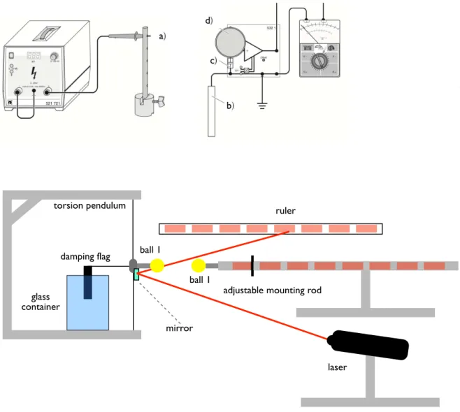
Torsion is a twisting resulting from an applied torque. In turn, torque is the tendency of a force to rotate an object about an axis. In this experiment, we will make measurements of the Coulomb force between two charged balls. One of the balls is mounted on a torsion pendulum (see figure 1.1), and we will measure the Coulomb force through the torque it exerts to rotate the pendulum.

The torsion pendulum can be modelled as a harmonic oscillator. Once oscillations have died out, the rotation of a pendulum from its rest position is

θ = ^F

^L

D , (1.3)

where F

is the applied torque, L is the distance from the pendulum wire to the centre of the ball (Ball 2 in figure 1.1), and D is the intrinsic restoring torque of the pendulum. For the tor- sion pendulums used in this experiment, D ≈ 3 · 10

Nm. The specific value of D measured for your torsion pendulum is written on the pendulum base. We make the assumption that the Coulomb force, F

acts as torque with 100% efficiency, i.e. that F

= F

.

We measure the rotation of the pendulum by reflecting a laser beam off a mirror that is at- tached to the pendulum. The laser beam then hits a ruler, and we can use simple trigonometry to determine changes in angle. It is important to note that the change in angle measured by the laser is twice the angle that the torsion pendulum rotates. That is, if the laser measures an angle α, then the rotation of the pendulum is θ = α/2.

1.3 Experiment

In this experiment, you will use a torsion pendulum to measure the force between two charged spheres, first as a function of the distance between the spheres and then as a function of their charge. From this, you will be able to derive the permittivity of the vacuum, ε

.

In order to make an absolute measure of the force between the spheres possible during the course of a standard lab, most of this experiment is already built up. The equipment is sen- sitive and precisely tuned, so please be careful with it! You will also be working with a high voltage power supply (25 kV!), which demands respect and care for safe working.

Although conceptually reasonably straightforward, this is one of the most difficult and tem- peramental experiments in the AP lab. It is therefore an excellent exercise in real-life lab work.

1ε₀=8, 854·10⁻¹² _Vm^As

4

The main issue is that the spheres can lose their charge quite quickly, with the rate of charge loss varying from day to day, e.g. due to the atmospheric conditions. This can result in quite a severe experimental difficulty, and the resulting data is generally quite noisy. Although frus- trating, is important not to despair! Repeat your measurements many times, average your data, and you will find signals that you can analyse.

a)

b) c) d)

torsion pendulum

damping flag

glass container

ball 1

ball 1

adjustable mounting rod

mirror

laser ruler

Figure 1.1: Top left: High voltage power supply and the high-voltage probe (a) used to charge the metal balls. Top right: electrometer amplifier circuit, with multimeter, used to measure the charge on the balls. Labels indicate: b) discharge rod; c) capacitor; d) Faraday cup (view from top). Bottom: Schematic of the experimental setup, showing the torsion pendulum, the two balls, the laser and the ruler which is to measure the deflection of the Torsion.

Torsionswaage = torsion pendulum. Dämpfungsfahne = damping flag. Wasserbad = glass container (for water). Kugel 1/2 = ball 1/2. Spiegel = mirror. Masstab = ruler. Ausfahrarer Masstab = adjustable mounting rod.

1.3.1 Equipment

1.3.2 Experimental Procedure

• Check that all the required equipment is there (see 1.3.1). Have a think about how you are going to position the various pieces of equipment, e.g. the stand for the Ball 1.

Discuss this with the experiment supervisor

• Connect the two high-voltage supplies with the electrometer amplifier (as shown in pic- ture 1.1).

• Fill the glass container with water and carefully insert the damping-flag (picture 1.1).

Check that the motion of the flag is not obstructed by the walls of the glass container.

5

Component Number

Laser 1

Power Supply 2

High Voltage Source 2

Torsion pendulum 1

Electrometer Amplifier 1

Balls 3

1 m Ruler mounted on a tripod 1 Tripod for distance measurement 1

Multimeter 1

As the glass container is somewhat small, you will probably have to adjust its position depending on whether the spheres are attracting or repelling one another.

• Familiarise yourself with how to charge the balls. Turn on the high-voltage supply and set it to 15 kV. Gently touch the top of each ball in turn with the high-voltage device tip, then turn the high-voltage supply off. Be careful not to move the balls when charging them: the only motion should be due to the Coulomb force.

• Familiarise yourself with measuring the rotation angle of the torsion pendulum. Adjust the ruler and laser so that you can make measurements for a reasonable range of angles.

Note down the position of the laser point on the ruler (the zero-point), and measure the distance from the mirror to the ruler. If you move the laser or ruler during the experi- ment, you need to measure the zero-point and mirror-ruler distance again. Charge the balls, and observe how the laser point moves on the ruler. Estimate the uncertainty with which you can determine the maximum rotation angle.

• Calibration: In order to perform calculations using Coulomb’s law, we need to know the charge on each of the balls. The charge is determined by the setting that we choose on the high voltage power supply (5 kV, 10 kV, 15 kV etc), and should be linearly proportional to this setting: q ∝ V

, where q is the charge on a ball, and V

is the power supply voltage. The first step is therefore to perform a calibration, to determine the relationship between the power supply setting and the charge on the balls.

In principle, we should perform a calibration for each ball individually, as the exact relationship can be different for each. In practice, we can reasonably assume that the calibration factor will be very similar for both balls. It is easiest to perform the calibration on Ball 1 (mounted on the rod).

We measure the charge on a ball using the electrometer amplifier setup. The experiment supervisor will demonstrate how this works. Basically, you touch the discharge rod (shown in figure 1.1) to the ball, and the electrical potential energy, U, stored by the excess charge on the ball is display in [V] on the multimeter. U is related to the charge by the capacitance of the amplifier circuit, C (either 1 nF or 10 nF):

q = C · U (1.4)

By measuring q for various values of V

, you can construct a calibration curve. A rea- sonable set of points to measure at would be (5 kV, 10 kV, 15 kV, 20 kV, 25 kV). Between measurements, make sure that you discharge the balls between by touching them with the discharge rod. You will use the calibration curve in the rest of the experiment to

6

convert the values of V

set on the power supply to the charges on the balls, q

and q

. It is recWerteommended to take the first measurements using 15 kV, as the measure- ments are harder at both low voltage (small signal) and high voltage (electrical charging of nearby objects - see (2+3) below).

Complications:

1) Charge loss with time. The charge on the balls does not stay there for ever, and even- tually leaks out to the environment. This occurs through various channels, including loss directly to the atmosphere. The loss rate is therefore a function of the weather, and varies day-to-day. In general, it is quite short, on the order of a few seconds. One impor- tant consequence is that it is important to measure the charge on the balls at a fixed time after charging them (e.g. 0.5 s after charging - you should play with this delay to opti- mise it for the conditions on your day). A second consequence is that it is possible that you will not measure any charge on the balls for low values of V

. This is because the charge has already dropped below the detection threshold by the time you measure it.

2) The high voltage supply is strong enough to induce a signal in the electrometer am- plifier circuit even when the high voltage tip is far away. It is therefore important to ground the discharge rod to the Faraday cup whilst charging the balls. To measure the charge on the balls, turn the power supply off before taking the discharge rod away from the Faraday cup.

3) The glass container (and possibly other parts of the experiment) will often also build up a charge over time. Discharge this by rubbing the glass walls (or other parts of the ex- periment) with the discharge rod. Note that as the glass is not a conductor, you need to rub the rod over the entire glass surface (or most of it) to achieve an effective discharge.

You can also put the discharge rod in the water in case it has also built up charge. The walls should be discharged frequently - after every measurement is safest, though it will probably be ok to discharge after every 2-3 measurements. You should also perform this discharging during the measurements as a function of sphere separation and charge.

4) Noisy data. The result of (1-3) is that there is likely to be a large amount of scatter in your measurements. In addition to taking the steps outlined in (1-3), you will need to take several repeated measurements and average them together. Depending on the level of noise (which varies day-to-day), 5-10 measurements at each V

setting should be sufficient. If the data is particularly noisy, you might need 20 repeated measurements.

When plotting the data, you should plot both the mean value of the repeated measure- ments, and error bars determined by their standard deviation.

• Measurement as a function of sphere separation: This part of the experiment is per- formed with equal charge on both of the spheres. You will get the strongest interaction between the spheres if you set the high-voltage supply to 25 kV. Depending on the day, however, this may lead to an unacceptable amount of inductive interference and noise.

15 kV is a more reliable setting.

Play with the position of Ball 1 to find the range of separation distances over which you should perform the measurement. The upper limit on separation distance should be a distance slightly further than that for which you can detect a force between the two balls.

The lower distance is

7

For each measurement, begin by charging each ball and then switching off the power supply. Then write down the maximum distance the laser point moves from the zero- point on the ruler. Between measurements, make sure that you discharge the balls be- tween by touching them with the discharge rod.

Take measurements at 8-10 different distances. At each distance, repeat your measure- ment 5-20 times, depending on how noisy the experiment is on the day. At the largest distance, you should be able to only barely detect any interaction between the two balls.

The closest distance is limited by noise induced by the high voltage tip, and is typically

around 1-2 cm.

• Measurement as a function of the charges q

and q

: This part of the experiment is performed at a fixed separation distance. The charge on Ball 2 is fixed, and the charge of Ball 1 is varied. Both charges are of the same sign.

The balls should be positioned close enough that you have a large signal, but far enough apart that charging one ball does not significantly perturb the charge on the other ball.

A typical distance is around 5 cm, but you should optimise this to the conditions on the day.

You need two power supplies. Use one to charge Ball 2 with 15 kV. Use the other to charge Ball 1 with a varying voltage: 10 kV, 12.5 kV, 15 kV, 17.5 kV, 20 kV. For each different voltage, repeat your measurement 5-20 times, depending on how noisy the experiment is on the day. Between measurements, make sure that you discharge the balls between by touching them with the discharge rod.

1.4 Evaluation

When plotting data, you should plot both the mean value of the repeated measurements, and error bars determined by their standard deviation.

• Calibration: Using Eq. 1.4, take the measurements of charge on the ball that you mea- sured using the multimeter and convert them from measured voltage, U, to charge on the balls, Q.

Plot the calibration data in the form of charge, Q, as a function of charging voltage, V.

Perform a linear fit to the data, Q = aV + b. If the data is only linear for larger values of V (e.g. if Q = 0 for V < 10 kV), then you should only perform the fit to the linear region. You can now use the fit values a and b to calibrate your data for the rest of the experiment.

• Measurement as a function of sphere separation: Calculate the force from the deflec- tion of the torsion pendulum. Use the formulas given in the theory section, and don’t forget the factor of two in the laser deflection. Construct a plot of your data as F ( r ) (force as a function of distance) and fit the function F ( r ) = ar

+ b. Is your data consistent with the distance-relationship that appears in Coulomb’s law? Can you confirm this dis- tance relationship, or are other distance relationships also consistent with the data? Fit

2Approximately - check for yourself! The closer you can measure, and the more points you measure at, the easier the analysis becomes.

8

the data with the following three functions: (1) F ( r ) = ar + b (linear); (2) F ( r ) = ar

+ b (inversely proportional); (3) F ( r ) = A exp (− ar ) + b (exponential). Discuss your results, and compare the four fits. All four fits should be shown overlaid on a single plot, so that they can be directly compared to one-another and the data.

• Measurement as a function of the charges q

and q

: Plot your data in the form of force as a function of charge (F ( q ) ). Fit a straight line to the data. Determine ε

from the slope of this line, using Eq. 1.1.

Compare your results with the literature value of ε

and discuss. If the value you obtain for ε

isn’t what you expected, have a think about why. Discuss why it could be big- ger or smaller than the literature value, given the experimental issues you faced. You should make reference to your equation for ε

, and the measured values you input. For example, if you overestimate q in your measurements, does this result in an over- or underestimation of ε

?

Notes on Experiment Reports

• UNITS! There is no excuse for failing to include the units in your calculations and results.

Do not write the charge as q

= 0.4, or report a value ε = 8 × 10

.

• You should find a vector drawing program that you like and use it for diagrams and schematics (e.g. the experiment setup). Inkscape is a pretty decent option, and is also free.

• Label all figures. Describe what they are showing, which data you’re plotting, etc in a caption.

• Make figures big enough to read - they should cover a significant fraction of the page width.

• Figures, tables, equations etc should also be discussed in the text. It is NEVER ok to include one of these without also discussing it in the main body

• For diagrams of the experiment apparatus / setup, remember to include the things you were measuring, eg the angle alpha, the distance between the spheres, etc. Don’t forget to also introduce these parameters in the text.

• Use a sensible number of significant figures. The exact number is determined by your experimental uncertainty. If you calculate a charge with uncertainty ± 0.1 C, write Q = 4.1 C, not Q = 4.1214353434509 C.

• For uncertainties, always write down where you are getting your uncertainty value from - e.g. estimated as half the limit of reading of the ruler, or estimated as your ability to align two components together.

• For the Introduction/Theory section (and others as well): Tell a story! Write as if you are explaining the experiment to one of your peers, i.e. someone who is familiar with physics, but not at all with the particular theory you are using or the experiment you are doing. A common mistake is to not provide sufficient context/explanation, and just to throw a few relevant equations at the page. This isn’t enough. Also, avoid including

9

irrelevant information simply because it is in the theory section of this lab manual. A good theory section will bring everything together, and explain why you are doing what you are doing, why you are using the equations you are using, etc - i.e. why, not just what.

• UNITS!

Literature

• Demtröder Band 2 - Elektrizität und Optik, 6. Auflage: Abschnitt 1.1 bis 1.3

10