Median, Mean, and Variance Stability of a Process under Temporally Correlated Stochastic Feedback

Research Collection

Journal Article

Median, Mean, and Variance Stability of a Process under Temporally Correlated Stochastic Feedback

Author(s):

Smith, Roy; Bamieh, Bassam Publication Date:

2021-07

Permanent Link:

https://doi.org/10.3929/ethz-b-000438673

Originally published in:

IEEE Control Systems Letters 5(3), http://doi.org/10.1109/LCSYS.2020.3006726

Rights / License:

In Copyright - Non-Commercial Use Permitted

This page was generated automatically upon download from the ETH Zurich Research Collection. For more information please consult the Terms of use.

ETH Library

Median, Mean, and Variance Stability of a Process under Temporally Correlated Stochastic Feedback

Roy S. Smith and Bassam Bamieh

accepted for publication: IEEE Control Systems Letters, Vol.5, Issue 3, July 2021 (DOI: 10.1109/LCSYS.2020.3006726) c2021 IEEE

Abstract—Stochasticity in feedback gains leads to heavy-tailed state distributions in which the median, mean, and variance have different stability properties. These properties are characterised for a scalar system with temporally correlated stochastic feed- back. Necessary and sufficient conditions are obtained for the generic case of log-normal feedback gain distributions. Temporal correlation is modeled by a multivariable Gaussian distribution of the logarithm of the feedback gain values. This correlation has no effect on the stability of the median of the state, but does influence the stability of both the mean and the variance of the state. Examples illustrate both stabilising and destabilising correlations.

Index Terms—Stochastic systems, Stability of linear systems, Time-varying systems.

I. I

NTRODUCTION

D YNAMICAL systems with stochastic coefficients arise in many physical models which are either imprecisely known or operate in inherently stochastic environments.

Stochasticity in parameters is fundamentally different from stochastic exogenous inputs that enter additively as forcing functions for example. One way to appreciate the difference is to note that stochastic system parameters are actually stochastic feedback loops inside the system description. As is well known, feedback affects dynamical systems in funda- mentally different ways than additive exogenous disturbances.

Stochasticity in feedback gains also arises in data-based con- trol methods due to the inevitable noise in the data. Similar dynamics arise in financial systems and statistical mechanics.

Most classical stochastic control theory deals with the case of additive, exogenous inputs. If the dynamics are linear and one is interested only in second order processes, then there is no “closure problem”, and covariance analysis is sufficient to quantify the system behaviour. However, if one is interested in quantities other than first and second order moments, or if the exogenous inputs are not Gaussian, then these classical methods are not applicable. In the setting where feedback gains are stochastic, there is yet another phenomenon where even if a linear system’s parameters are Gaussian processes, the state evolution involves the products of a stochastic state and a stochastic gain, leading to heavy-tailed state distributions.

This research is partially supported by NSF Awards CMMI-1763064 and ECCS-1932777.

R. Smith is with the Automatic Control Lab., ETH Zürich, Switzerland, (rsmith@control.ee.ethz.ch).

B. Bamieh is with the Mechanical Engr. Dept., Univ. California, Santa Barbara, USA, (bamieh@engineering.ucsb.edu).

Thus linear systems with stochastic feedbacks can exhibit a very rich phenomenology of behaviors.

This problem was studied in a control context in [1] and [2].

The proof that the limiting distribution is a heavy-tailed distribution appears in [3]. Some aspects of stability in discrete stochastic feedback systems were investigated in [4]. A more complete analysis from a feedback control point of view was given in our prior work [5].

All of the previous work considered the stochasticity to be independent and identically distributed (i.i.d.) between samples. One reason for imposing this assumption is mathe- matical tractability. The techniques used in the aforementioned references rely heavily on the i.i.d. assumption for the analysis to be tractable. There is in general no clear way to extend those analysis techniques to cases where stochastic gains are temporally correlated. This issue is not purely academic. There are many applications where one would need to introduce some notion of temporal correlation (correlation times) into the theory. The behaviour of various statistics of interest appear to depend on these temporal correlations. To put this issue in some context, consider the i.i.d. case one the one hand, and the case of time-constant, but randomly selected feedback gains on the other. They can be regarded as two extreme cases of a continuum of temporally correlated gains. The limit of short correlation times is conceptually the i.i.d. case, while the limit of long correlation times is the random constant case. These models are quite important in statistical physics where the long correlation times limit is referred to as the “quenched noise”

limit [6], and the short correlation times limit is the so-called

“annealed limit”. Such models are encountered in the physics of disordered systems, and in particular appear in the famous problem of Anderson localization [7]. This remains an active area of research given the complexity of the phenomenology that arises in seemingly simple models.

Our prior work [5] considered the i.i.d. stochastic feedback case, which was analysed using techniques that do not easily extend to the temporally correlated gains case. In this paper, we present one model of temporal correlations that appears to be tractable. We are able to quantify the behaviour of vari- ances, means and medians of stochastic gains with lognormal distributions and a special type of temporal correlation.

A. Notation

For a random variable a, a

∼

f

a

(a) denotes that it is drawn

from a probability distribution with a density function f

_a

(a).

z⁻¹

ak∼fa(a)

xk xk+1

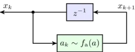
Fig. 1. Stochastic feedback system. At each time instant,k, a new sample a_k∼fa(a)is drawn from the distribution.

The expected value of a is

E

a

= µ

_a

and its variance is σ

_a²

. The normal distribution of mean µ and variance σ

²

is denoted by

N

(µ, σ

²

). Log-normal distributions are denoted by

LN

. If a symmetric matrix X is positive definite this is denoted by X 0. The i, 

^th

component of X is denoted by [X]

_i,j

. The N -length column vector of ones is denoted by

1N

.

II. M

ODEL AND PROBLEM FORMULATION

The plant is scalar system evolving with the dynamics, x

k+1

= a

k

x

k

, k = 0, 1, . . . . (1) The state variable a

k

is, at each time step, drawn from a distribution a

k ∼

f

a

(a). This can be viewed as the stochastic feedback structure given in Figure 1. It is a simple matter to consider more general first order systems with stochastic feed- back. It can also be equivalently formulated as multiplicative noise in a first order feedback system.

This is the same problem formulation as that considered in a prior paper [5] in the i.i.d. setting, where a very general class of distributions f

_a

(a) on positive support was considered.

In the current work the theoretical results are derived under the assumption that the feedback is drawn from a log-normal distribution, f

a

(a) . The log-normal distribution is defined by exponentiating a normally distributed random variable. If α

∼ N

(µ

α

, σ

_α²

), then the random variable defined by a = e

^α

is log- normally distributed, a

∼ LN

. The key feature here is that a log-normal distribution is closed under both multiplication and raising to a power.

The state of the system (1) after N time-steps is x

_N

= x

₀

N−1

Y

k=0

a

_k

, (2)

and without loss of generality it will be assumed that x

0

= 1.

As x

N

is the product of random variables, it is also a random variable. Furthermore, as a

k∼ LN

, the state x

N

is also a log- normal random variable, x

N ∼ LN

with mean and variance denoted by µ

xN

and σ

²_xN

respectively.

The question of stability can be posed in terms of a variety of statistical quantities and this paper is concerned with three definitions of stability:

a) Median stability: The system is median stable if,

N

lim

−→∞

median(x

N

) = 0.

b) Mean stability: The system is mean stable if, lim

N−→∞E

x

_N

= 0.

c) Variance stability: The system is variance stable if, lim

N−→∞Eh

x

N − E

x

N²i

= 0.

Necessary and sufficient conditions for all three stability conditions were derived in [5], under the assumption that the a

_k

were i.i.d. random variables. The current work restricts the consideration of a

_k

to log-normal variables, but removes the independence assumption. In contrast to the i.i.d. case, both the mean and variance stability depend strongly on the temporal correlation. However the stability of the median is unchanged by correlation of the a

k

random variable.

A. Analysis framework

The analysis of this system will proceed by taking the obvious step of working with the logarithm of a

k

and x

k

. By defining,

α

_k

= ln(a

_k

), and ζ

_k

= ln(x

_k

), the dynamics in (2) can be written instead as,

ζ

N

= ζ

0

+

N−1

X

k=0

α

k

. (3)

The definition of α

k

as the logarithm of the random variable a

k ∼ LN

implies that α

k ∼ N. As all of the

α

k

are normally distributed (and correlated in a manner detailed in Section II-C), and ζ

0

= ln(x

0

) = 0 by assumption, ζ

N

is also normally distributed.

The approach to be taken here is to characterise the correla- tion between the stochastic feedback variables a

k

, in terms of a correlation between the logarithmically transformed random variables α

k

. As all of the logarithmically transformed vari- ables are characterised in terms of sums of normal variables the stability conditions can be considered instead in terms of the ζ

_k

variables. Doing this requires more detail on the relationship between the normal and log-normal distributions.

To facilitate readability we will use Greek symbols for variables in the logarithmic domain (for example ζ

_k

and α

_k

) and the Latin alphabet for variables in the state and feedback domain (for example x

_k

and a

_k

).

B. Normal and Log-Normal distributions The monotonic variable relationship

ζ

_k

= ln(x

_k

),

will transform the median (and any percentile statistic) directly as,

Prob

{xk

< z} = Prob

{ln(xk

) < ln(z)}

= Prob

{ζk

< ln(z)} . Therefore,

median(ζ

_N

) = ln(median(x

_N

)) and

median(x

_N

) = e

^median(ζN)

. (4)

However the relationship between the means and variances is more complicated [8].

µ

α

= ln

µ

_a q

1 +

_µ^σa22 a

!

, (5)

σ

_α²

= ln

1 + σ

²_a

µ

²_a

, (6)

and

µ

_a

= e

^µα+σ2α/2

, (7) σ

_a²

=

e

^σα2 −

1 e

^2µα+σα2

. (8)

These relationships will be used to transform results from the ζ

N

domain to the x

N

domain and vice-versa.

C. Temporal correlation model

There are a variety of ways in which we can characterise the temporal correlation between the random variables, a

k ∼ LN

. The approach taken here is to characterise the correlation in terms of the normally distributed α

k∼ N

variables. We model the correlation between the α

k

random variables as the output of a linear time-invariant filter (denoted by Γ) driven by an i.i.d. Gaussian noise sequence. This implies that the vector

α =

α

₀ · · ·

α

_N−1T

(9) is modeled as coming from a multivariable Gaussian distribu- tion. This modeling choice gives a relatively straightforward characterisation of the median, mean, and variance stability conditions.

The log-domain filter Γ is specified by its pulse response, γ

τ

, τ = 0, 1, . . . ,

∞.

The model for each α

k

is therefore,

α

k

=

∞

X

τ=0

γ

τ

ν

_k−τ

, ν

_k−τ ∼ N

(µ

ν

, σ

²_ν

). (10) We assume (without loss of generality) that γ

0

= 1 and that Γ is stable. Note that (10) is the asymptotic limit, implying that the filter generating the α

_k

is already in equilibrium at time-step k = 0.

The appropriate choice of µ

_ν

and σ

_ν²

can be determined by calculating µ

_αk

and σ

²_αk

.

µ

_αk

=

E

" _∞ X

τ=0

γ

_τ

ν

_k−τ

#

=

∞

X

τ=0

γ

_τE

ν

_k−τ

= Γ(e

^j0

) µ

_ν

, where Γ(e

^j0

) denotes the zero frequency gain of the filter Γ.

By choosing

µ

_ν

= µ

_α

/Γ(e

^j0

),

the correlation model gives the appropriate value of µ

α

. To select σ

_ν²

we evaluate the variance of α

k

. As the variance scales with the square of the

H2

norm,

σ

_α²_k

=

∞

X

i=0

|γ_i|²

σ

_ν²

=

kΓk²₂

σ

_ν²

. (11) Therefore selecting

σ

_ν²

= σ

²_α

/kΓk

²₂

, (12)

Stability property

in terms of fa(a)distribution

in terms of fα(α)distribution median(xN) µ²_a−σ²_a/µ²_a<1 µα<0

mean(xN) µa<1 µα+σ_α²/2<0 variance(xN) µ²_a+σ²_a<1 µα+σ_α² <0

TABLE I

STOCHASTIC FEEDBACK GAIN STABILITY CONDITIONS FOR I.I.D. LOG-NORMAL DISTRIBUTIONSa∼ LN

will give the value of σ

²_α

required for the correlation model.

A similar calculation, using shifted indices, will give the covariances,

E

α

_i

α

_j

=

∞

X

m=0

γ

_m

γ

_m+j−i

!

σ

²_ν

. (13) The above results can also be expressed using a mul- tivariable Gaussian formulation for the length-N vector α defined in (9), giving α

∼ N

(µ

_αN

, Σ

_N

), where the diagonal components of the covariance matrix, Σ

N

, are given by (12), and the off-diagonal components are given by (13).

D. Temporal correlation in the Log-Normal domain

The filtered i.i.d. noise model for correlation (in (10)) that generates the vector α with correlated components has an equivalent representation in the original problem domain for generating the temporally correlated a vector. This can be determined by transforming (10) to the a domain and gives,

a

k

=

∞

Y

τ=0

(v

_k−τ

)

^γτ

,

where the i.i.d. log-normal random variable v

_k−τ

is defined by

v

k−τ

= e

^νk−τ

, ν

∼ N

(µ

ν

, σ

_ν²

).

The mean and variance of v

∼ LN

are given by applying the mapping in (7) and (8) to the mean and variance of ν

∼ N

(µ

ν

, σ

²_ν

).

This form of temporal correlation model is certainly not standard, but it does give a log-normal distribution a

_k

from a product of time shifted i.i.d. log-normal random variables raised to appropriate powers.

III. S

TABILITY RESULTS

The median, mean and variance stability conditions for this system with i.i.d. stochastic feedback were derived in [5]

and are summarised here for comparison. Table I illustrates the three stability conditions. Each of these stability criteria will now be considered for the temporal correlation model introduced in Section II-C.

The basis of the results is the calculation of the mean and variance of

α

N

=

N−1

X

k=0

α

k

.

The evolution of the mean of α

_N

is unaffected by the correlation between the α

_k

random variables,

E

α

_N

=

E

"_N−1 X

k=0

∞

X

i=0

γ

_i

ν

_k−i

#

=

N−1

X

k=0

∞

X

i=0

γ

_iE

ν

_k−i

= N Γ(e

^j0

)µ

_ν

= N µ

_α

. (14) To derive the variance of α

_N

note that

α

N

=

1

· · ·

1 α,

where α

∈ R^N

is the multivariable Gaussian vector defined in (9). The variance of α

N

is therefore given by,

variance(α

N

) = variance(1

^T_N

α) =

1^T_N

Σ

N1N

. (15) The median stability condition depends only on

E

α

N

as stated formally in the following.

Theorem 1: The stochastic feedback system specified in (1) is median stable under correlated log-normal feedback if and only if, µ

α

< 0.

Proof: As a is multivariable log-normal, α is multivariable normal and α

N

is normal, and so α

N

has median equal to its mean. Therefore, from (4) and (14),

median(x

N

) = e

^median(αN)

= e

^mean(αN)

= e

^{N µα}

, which goes to zero as N

−→ ∞

if and only if µ

α

< 0.

The mean and variance of x

_N

depend on both the mean and variance of α

_N

. Although the mean of α

_N

is unchanged by correlation, the variance is not. We therefore expect the conditions for mean and variance stability to depend on the correlation.

To quantify the dependency of the mean of x

_N

on correla- tion consider the following.

Γ(e

^j0

)

²

=

∞

X

m=0

γ

m

!²

=

∞

X

m=0

γ

m

!



∞

X

j=0

γ

j





=

∞

X

m=0

γ

m

∞

X

t=−m

γ

m+t

=

∞

X

t=−∞

∞

X

m=0

γ

m

γ

m+t

. (16) Theorem 2: The stochastic feedback system specified in (1) is mean stable under correlated log-normal feedback if and only if,

µ

_α

+ Γ(e

^j0

)

²

2kΓk

²₂

σ

²_α

< 0.

Proof: Consider the ratio, mean(x

N

)

mean(x

_N−1

) = e

^ln

µxN

µxN−1

.

The following will show that, in the limit, the exponent is constant. In which case the conditions under which the exponent is negative are equivalent to the mean stability of x

N

. To this end consider,

ln

µ

x_N

µ

_xN−1

= ln (µ

_xN

)

−

ln µ

_xN−1

Observe that

µ

x_N

= e

^{N µα+121TNΣN1N}

. (17) Using the analogous result for µ

x_N−1

implies that,

ln

µ

x_N

µ

_xN−1

=

µ

α

+ 1 2

1^T_N

Σ

N1N − 1^T_N−1

0

Σ

N

1_N−1

0

. The term in parentheses is simply the sum of the elements N

^th

row of Σ

_N

and of the elements of the N

^th

column of Σ

_N

, less the Σ

_N,N

element. This is therefore equal to

µ

α

+ 1 2

N

X

l=1

[Σ

N

]

N,l

+

N−1

X

n=1

[Σ

N

]

n,N

!

.

From (13) this can be expressed in terms of the pulse response coefficients of Γ as

µ

α

+ σ

²_ν

2

N

X

l=1

∞

X

m=0

γ

m

γ

_m+l−N

+

N−1

X

n=1

∞

X

m=0

γ

m

γ

m+N−n

!

.

Now define an index t = l−N for the first sum and t = N

−n

for the second. Note that t ranges from

−N

+ 1 to 0 in the first summation pair and from 1 to N−1 in the second. These contiguous ranges can be combined to give,

µ

α

+ σ

_ν²

2

N−1

X

t=−N+1

∞

X

m=0

γ

m

γ

m+t

!

.

In the limit as N

−→ ∞, equation (16) shows that the term in

parentheses converges to Γ(e

^j0

)

²

. Substituting (12) gives the required condition.

Observe that in the uncorrelated case Σ

N

= σ

_ν²

I = σ

²_α

I, and Γ(e

^j0

)

²

/kΓk

²₂

= 1. In this case Theorem 2 is equivalent to the condition for mean stability given in Table I. The mean of x

N

for any finite N can be calculated directly from (17). This calculation is used in the illustrative examples in Section IV.

The condition for variance stability can also be stated in terms of the mean and variance of f

_α

(α) and the gains associated with the correlation filter Γ.

Theorem 3: The stochastic feedback system specified in (1) is variance stable under correlated log-normal feedback if and only if,

µ

α

+ Γ(e

^j0

)

²

kΓk²₂

σ

_α²

< 0.

Proof: From (8), the variance of x

_N

is σ

_x²_N

=

e

^σαN2 −

1 e

^{2µαN+σαN2}

.

From (14), µ

αN

= N µ

α

. The argument in the proof of Theorem 2 shows that the asymptotic variance of α

N

with respect to N is,

N−→∞

lim σ

²_αN

= N Γ(e

^j0

)

² kΓk²₂

σ

_α²

.

Label Filter Γ(e^j0)² µα σ_α² µa

Case 1a i.i.d. — -0.1 0.3 1.05

1b Γ1 0.09 -0.1 0.3 1.05

Case 2a i.i.d. — -0.1 0.1 0.95

2b Γ2 7.29 -0.1 0.1 0.95

TABLE II

SIMULATION EXAMPLE CASE STUDY CONFIGURATIONS

Therefore

N−→∞

lim σ

²_xN

=

e

^{N σ2αΓ(ej0)2/kΓk22}−

1 e

^{2N µα+N σα2Γ(ej0)2/kΓk22}

= e

^{2N(µα+σ2αΓ(ej0)2/kΓk22)}−

e

^{2N(µα+σ2αΓ(ej0)2/2kΓk22)}

. The exponent of the first term is larger than the that of the second and so determines whether or not the limit goes to zero. Convergence to zero as N

−→ ∞

occurs if and only if the exponent of the first term is negative.

IV. I

LLUSTRATIVE EXAMPLES

Two examples of correlated stochastic feedback are used to illustrate the effects of temporal correlation. As introduced in Section III, the correlation is modeled in the logarithmic variable domain as a causal LTI filter driven by a normally distributed i.i.d. random variable. We present two case exam- ples and for each compare the effect of correlated α

k

variables with independent α

k

variables. The details of the two cases are summarized in Table II.

For simplicity we compare two FIR filters, specified here by their pulse responses,

Γ

₁

: γ

₁

(k) =

1.0

−0.9

0.2

−0.6

0

· · ·

and

Γ

₂

: γ

₂

(k) =

1.0 0.9 0.2 0.6 0

· · ·

. Each has the same 2-norm scaling,

kΓk²₂

= 2.21, but differ in their zero frequency gains (see Table II).

Figure 2 illustrates multiple sample trajectories generated by (1) with a

k

= e

^αk

generated with the mean and variance given for Case 1a in Table II. As

µ

_a

= e

^µα+σ2α/2

= 1.05 > 1,

the mean of x

_N

(blue dashed line) grows exponentially.

However µ

_α

=

−0.1

< 0 and so the median of x

_N

(magenta dashed line) decays to zero. This is a case where the system has a stable median and an unstable mean. The simulations are run for up to N = 50 and it is clear that the sample estimate of the mean (red solid line) deteriorates as N increases. This is because the stable median implies that the probability of a sample trajectory exceeding the mean decays exponentially to zero as N increases (see [5] for details).

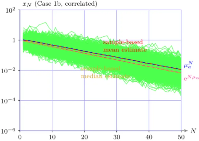
Figure 3 illustrates Case 1b where the mean and variance of α

k

are the same as Case 1a, but the α

k

are now correlated.

From Theorem 2 the low value of Γ

1

(e

^j0

) leads to mean stability. In this case both the median and mean decay to zero with different exponents.

xN (Case 1a, i.i.d.)

sample-based median estimate

sample-based mean estimate

10⁻⁶ 10⁻⁴ 10⁻² 1 10²

N

0 10 20 30 40 50

e^{N µα} µ^N_a

Fig. 2. Simulations (1,000 realisations) of Case 1a trajectories. The random variablea_k∼ LN is i.i.d. The theoretical and sample medians, as well as the theoretical and sample means, are shown. The median is stable and the mean is unstable.

xN (Case 1b, correlated)

sample-based median estimate

sample-based mean estimate

10⁻⁶ 10⁻⁴ 10⁻² 1 10²

0 10 20 30 40 50 N

e^{N µα} µ^N_a

Fig. 3. Simulations of Case 1b trajectories. The correlation is modeled by theΓ1 filter in theαk ∼ N(µα, σ_α²)domain. The theoretical and sample medians, as well as the theoretical and sample means, are shown. The median are the mean are both stable.

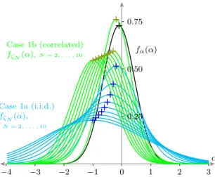
The differing stability cases can also be examined by looking at the evolution of the probability density functions of ζ

N

and x

N

. Figure 4 illustrates the evolution of these densities for the first N = 10 steps in Cases 1a and 1b. For N = 0, both the i.i.d. and correlated cases have the same initial density. For both cases the evolution of the mean of ζ

N

is identical—correlation does not affect median stability.

However correlation modifies the variance of α

N

—in this case significantly reducing its growth with N. This is also clear from the spread of sample trajectories illustrated in Figure 3.

The effect of the variance reduction in the ζ

N

domain on

the mean of x

N

is illustrated in Figure 5. All distributions

shown are log-normal distributions—the key issue here is the

evolution of the median and the mean as a function of N . In

the i.i.d. case the mean of x

N

(blue +) grows with N, while

the median (blue circles) decays to zero. In the correlated case

the median of x

N

(olive circles) is the same as the i.i.d. case,

but the mean of x

N

(olive +) decays to zero. Figures 2 to 5

illustrate that the correlation in Case 1 stabilises the mean of

x

_N

while leaving its median unchanged.

α 0.25

0.50 0.75

−4 −3 −2 −1 0 1 2 3

fα(α) Case 1b (correlated)

fζN(α),^N= 2, . . . ,10

Case 1a (i.i.d.) fζN(α),

N= 2, . . . ,10

Fig. 4. Evolution of the probability density functions in theαkdomain for Case 1. The black line shows the distribution of theα∼ N(µα, σ²_α)variable.

The cyan plots show the evolution ofζN distribution forN= 2, . . . ,10in the i.i.d. case. The green plots show the evolution ofζN distribution in the temporally correlated (usingΓ1) case. Means of each distribution are shown by+.

0 a 0.5 1.0 1.5 2.0 2.5

0 0.5 1 1.5 2

fa(a) Case 1b (correlated) fx_N(a), N= 2, . . . ,10

Case 1a (i.i.d.) fx_N(a), N= 2, . . . ,10

Fig. 5. Evolution of the probability density functions in theak domain for Case 1. The black line shows the distribution of thea∼ LN variable. The cyan plots show the evolution of thexNdistribution forN = 2, . . . ,10in the i.i.d. case. The green plots show the evolution of thex_Ndistribution in the correlated (usingΓ1) case. The means of each distribution are shown by +and the medians by circles.

Figure 6 illustrates the evolution of x

N

distributions for Case 2. The effect of the correlation in Case 2 is the opposite of that in Case 1; The mean of x

N

for i.i.d. feedback gains is stable, and is destabilised by correlated feedback gains.

The differences between the correlation filters is illustrated via their frequency responses in Figure 7. The stability criteria for the mean of x

N

is determined by the ratio, Γ(e

^j0

)

²

/kΓk

²₂

. For i.i.d. feedback gains this factor is one. For the correlated feedback in Case 1b the ratio is less than one, whereas in Case 2b it is larger than one.

V. C

ONCLUSION AND DISCUSSION

We have provided necessary and sufficient conditions for the median, mean, and variance stability of the state of a scalar system under temporally correlated stochastic feedback.

The condition for the stability of the median is unaffected

0 a 0.5 1.0 1.5 2.0 2.5

0 0.5 1 1.5 2

fa(a) Case 2b (correlated)

fx_N(a), N= 2, . . . ,10

Case 2a (i.i.d.) fx_N(a), N= 2, . . . ,10

Fig. 6. Evolution of the probability density functions in thexdomain for Case 2. In this case the i.i.d. evolution of x_N has a stable median (blue circles) and a stable median (blue+). The evolution for the correlated case shows a stable median (olive circles) but an unstable mean (olive+).

ω[rad/sec]

0 0.3 1.0 2.0 2.7

0 π/4 π/2 3π/4 π

Γ₁(e^jω)

Γ₂(e^jω)

Fig. 7. Frequency domain comparison of theα-domain temporal correlation filters,Γ1 and Γ2. Both filters havekΓk²₂ = 2.21. The DC gains of each filter are marked by circles.

by correlation. Correlation is modeled via an LTI filter in the log domain of the feedback gain. The stability of the mean and the variance of the state is determined by properties of this filter. In particular a high pass filter (more precisely a small Γ(e

^j0

)

²

/kΓk

²₂

ratio) has a stabilising effect on the mean and the variance. In contrast a low-pass filter (high Γ(e

^j0

)

²

/kΓk

²₂

ratio) has a destabilising effect. The heuristic interpretation is that with a low-pass filter, the destabilising effects of variance persist longer than in the high-pass case, leading to destabilisation with a lower variance. In the high- pass filter case subsequent correlated feedback gains tend to have the opposite sign reducing the destabilising effect of the variance.

R

EFERENCES

[1] K. Åström, “On a first-order stochastic differential equation,”Interna- tional Journal of Control, vol. 1, no. 4, pp. 301–326, 1965.

[2] J. C. Willems and G. L. Blankenship, “Frequency domain stability criteria for stochastic systems,” IEEE Trans. Automatic Control, vol. AC-16, no. 4, pp. 292–299, 1971.

[3] H. Kesten, “Random difference equations and renewal theory for products of random matrices,”Acta Math., vol. 131, pp. 207–248, 1973.

[4] M. Milisavljevi´c and E. I. Verriest, “Stability and stabilization of discrete systems with multiplicative noise,” in Proc. European Control Confer- ence, 1997, pp. 3503–3508.

[5] R. S. Smith and B. Bamieh, “Stochasticity in feedback loops; great expectations and guaranteed ruin,” IEEE Control Systems Magazine, 2020, (in press), arXiv preprint: 1912.08267.

[6] J. Toner, N. Guttenberg, and Y. Tu, “Swarming in the dirt: Ordered flocks with quenched disorder,” Physical review letters, vol. 121, no. 24, p.

248002, 2018.

[7] E. Abrahams,50 years of Anderson Localization. World Scientific, 2010.

[8] D. Finney, “On the distribution of a variate whose logarithm is normally distributed,” Supplement to J. Royal Statistical Soc., vol. 7, no. 2, pp.

155–161, 1941.