The Carbon Kuznets Curve: A Cloudy Picture Emitted by Bad Econometrics?

IHS Economics Series Working Paper 197

November 2006

The Carbon Kuznets Curve: A Cloudy Picture Emitted by Bad Econometrics?

Martin Wagner

Impressum Author(s):

Martin Wagner Title:

The Carbon Kuznets Curve: A Cloudy Picture Emitted by Bad Econometrics?

ISSN: Unspecified

2006 Institut für Höhere Studien - Institute for Advanced Studies (IHS) Josefstädter Straße 39, A-1080 Wien

E-Mail: o ce@ihs.ac.atffi Web: ww w .ihs.ac. a t

All IHS Working Papers are available online: http://irihs. ihs. ac.at/view/ihs_series/

This paper is available for download without charge at:

https://irihs.ihs.ac.at/id/eprint/1736/

The Carbon Kuznets Curve:

A Cloudy Picture Emitted by Bad Econometrics?

Martin Wagner

197

Reihe Ökonomie

Economics Series

197 Reihe Ökonomie Economics Series

The Carbon Kuznets Curve:

A Cloudy Picture Emitted by Bad Econometrics?

Martin Wagner November 2006

Institut für Höhere Studien (IHS), Wien

Institute for Advanced Studies, Vienna

Contact:

Martin Wagner

Department of Economics and Finance Institute for Advanced Studies Stumpergasse 56

1060 Vienna, Austria : +43/1/599 91-150 fax: +43/1/599 91-163

email: martin.wagner@ihs.ac.at

Founded in 1963 by two prominent Austrians living in exile – the sociologist Paul F. Lazarsfeld and the economist Oskar Morgenstern – with the financial support from the Ford Foundation, the Austrian Federal Ministry of Education and the City of Vienna, the Institute for Advanced Studies (IHS) is the first institution for postgraduate education and research in economics and the social sciences in Austria.

The Economics Series presents research done at the Department of Economics and Finance and aims to share “work in progress” in a timely way before formal publication. As usual, authors bear full responsibility for the content of their contributions.

Das Institut für Höhere Studien (IHS) wurde im Jahr 1963 von zwei prominenten Exilösterreichern – dem Soziologen Paul F. Lazarsfeld und dem Ökonomen Oskar Morgenstern – mit Hilfe der Ford- Stiftung, des Österreichischen Bundesministeriums für Unterricht und der Stadt Wien gegründet und ist somit die erste nachuniversitäre Lehr- und Forschungsstätte für die Sozial- und Wirtschafts- wissenschaften in Österreich. Die Reihe Ökonomie bietet Einblick in die Forschungsarbeit der Abteilung für Ökonomie und Finanzwirtschaft und verfolgt das Ziel, abteilungsinterne Diskussionsbeiträge einer breiteren fachinternen Öffentlichkeit zugänglich zu machen. Die inhaltliche Verantwortung für die veröffentlichten Beiträge liegt bei den Autoren und Autorinnen.

Abstract

In recent years many empirical studies of environmental Kuznets curves employing unit root and cointegration techniques have been conducted for both time series and panel data.

When using such methods several issues arise: the effects of a short time dimension, in a panel context the effects of cross-sectional dependence, and the presence of nonlinear transformations of integrated variables. We discuss and illustrate how ignoring these problems and applying standard methods leads to questionable results. Using an estimation approach that addresses the second and third problem we find no evidence for an inverse U- shaped relationship between GDP and CO2 emissions.

Keywords

Carbon Kuznets Curve, panel data, unit roots, cointegration, crosssectional dependence, nonlinear transformations of regressors

JEL Classification

C12, C13, Q20

Comments

The comments of Klaus Neusser, Georg Müller-Fürstenberger, and Reto Tanner are gratefully

Contents

1 Introduction 1

2 The Carbon Kuznets Curve 5 3 Panel Unit Root Tests 7

3.1 First Generation Tests ... 8 3.2 Second Generation Tests ... 12 3.3 Conclusions from Panel Unit Root Analysis ... 16

4 Panel Cointegration Tests 17 5 Estimation of the Carbon Kuznets Curve with Panel

Cointegration Methods and Using De-factored

Observations 21

5.1 Panel Cointegration Estimation... 21 5.2 Estimation with De-Factored Observations... 23

6 Summary and Conclusions 24

References 26 Appendix: Data and Sources 32

Appendix B: Bootstrap Algorithms 33

1 Introduction

Besides nuclear energy, hydrocarbon deposits like petroleum, coal and natural gas are cur- rently the only available large scale primary energy sources. Their utilization as fossil fuels leads to the emission of – amongst other pollutants – CO

, which is considered the principal anthropogenic greenhouse gas. Since most economic activities require the use of energy, a link between economic activity and CO

emissions appears plausible.

Increased atmospheric CO

concentration can persist up to thousands of years. It exerts a warming influence on the lower atmosphere and the surface, i.e. it initiates climate change, see Peixoto and Ort (1992) or Ramanathan, Cicerone, Singh, and Kiehl (1985). Rational and efficient climate policy requires reliable understanding and accurate quantification of the link between economic activity and CO

emissions.

In this paper we are concerned with the econometric analysis of the relationship between GDP and emissions. The core of the econometric approach to study the link between GDP and CO

emissions usually consists of estimating a reduced form relationship on cross-section, time series or panel data sets. Estimation techniques as well as variables chosen vary substantially across studies. Most of the studies focus on a specific conjecture, the so-called ‘Environmental Kuznets Curve’ (EKC) hypothesis. This hypothesis claims an inverse U–shaped relation between (the logarithm of per capita) GDP and pollutants. In the specific case of CO

emissions we speak of the ‘Carbon Kuznets Curve’ (CKC).

The EKC hypothesis has been initiated by the seminal work of Gene Grossman and Alan Krueger (1991, 1993, 1995). They postulate, estimate and ascertain an inverse U–

shaped relationship between measures of several pollutants and per capita GDP.

Summary discussions of this empirical literature are contained in Stern (2004) or Yandle, Bjattarai, and Vijayaraghavan (2004), who find more than 100 refereed publications of this type.

1Note that also specifications in levels instead of logarithms are used in the literature.

2To be precise, Grossman and Krueger actually use a third order polynomial in GDP whereas the quadratic specification seems to have been initiated by Holtz-Eakin and Selden (1995).

3A prominent alternative approach to study the links between economic activity and environmental dam- ages in general or emissions in particular is given by ‘Integrated Assessment Models’, pioneered with DICE of Nordhaus (1992) or MERGE by Manne, Mendelsohn, and Richels (1995). This approach consists of spec- ifying and calibrating a general equilibrium model of the world economy. The economic model is then linked with a climate model to integrate the effects of climate change feedbacks into the economic analysis. To a certain extent the econometric and the integrated assessment model approach can be seen as complements.

Unfortunately, only few authors have tried to combine the two approaches, see McKibbin, Ross, Shackleton, and Wilcoxen (1999) for one example. M¨uller-F¨urstenberger and Wagner (2006) contains a discussion on the relation or lack thereof between reduced form econometric findings and relationships derived with structural models.

In the empirical EKC literature there is an ongoing discussion on appropriate specification and estimation strategies, see Dijkgraaf and Vollebergh (2005) for a comparative discussion of econometric techniques applied in the literature. It is the aim of this study to contribute to this discussion by addressing several serious econometric problems that have not been appropriately handled or have been ignored to a certain extent up to now. We focus on parametric approaches only. For non-parametric EKC approaches (see e.g. Millimet, List, and Stengos, 2003), semi-parametric approaches (see e.g. Bertinelli and Strobl, 2005) or versions based on spline interpolation (see e.g. Schmalensee, Stoker, and Judson, 1998). To illustrate our arguments, we present computations for a panel data set for the Carbon Kuznets Curve comprising 107 countries (see Table 7 in Appendix A) over the period 1986–1998.

The discussion is on two – related – levels. The first level is a fundamental discussion on whether the time series and panel EKC literature is applying the appropriate tools. The second level is the issue whether the tools applied – abstracting from the first level issue of appropriateness – are applied correctly or with enough care. Of course, those two issues are related and there will be substantial overlap in the two levels of discussion. We turn to both issues below, but can already present the main observation here: The answer is rather negative on both levels.

When using time series or panel data the issue of stationarity of the variables is of prime importance for econometric analysis. This is due to the fact that the properties of many statistical procedures depend crucially upon stationarity or unit root nonstationarity, i.e.

integratedness, of the variables used. Related to this issue is the question of spurious re- gression (see e.g. Phillips, 1986) versus cointegration, see the discussion below. One part of the literature, in particular the early literature, completely ignores this issue, see e.g. Gross- mann and Krueger (1991), Grossmann and Krueger (1995), Holtz-Eakin and Selden (1995) or Martinez-Zarzoso and Bengochea-Morancho (2004) to name just a few.

Another part of the literature is mentioning the stationarity versus unit root nonstation- arity issue, these include inter alia Perman and Stern (2003), Stern (2004); and when allowing also for breaks Heil and Selden (1999) or Lanne and Liski (2004) (the latter in a time series context) are two examples. The problem is, however, that three important issues – on both levels of our discussion - have been ignored thus far. On the first level these are the following

4Two further empirical issues are neglected in this paper, since they are in principle well understood. These are the homogeneity of the relationship for large heterogeneous panels and the question of stability of estimated relationships.

two – given that the variables are indeed unit root nonstationary. First, the usual formula- tion of the EKC involves squares or even third powers of (log) per capita GDP. If (log) per capita GDP is integrated, then nonlinear transformations of it, as well as regressions involving such transformed variables, necessitate a different type of asymptotic theory and also lead to different properties of estimators. Regression theory with nonlinear transformations of integrated variables has only recently been studied in Chang, Park, and Phillips (2001), Park and Phillips (1999) and Park and Phillips (2001). Currently no extension of these methods to the panel case is available, which posits a fundamental challenge to the empirical EKC literature.

To our knowledge this nonlinearity issue has not been discussed at all in the EKC literature. One study avoiding the above problems is given by Bradford, Fender, Shore, and Wagner (2005). These authors base their results, using the Grossman and Krueger (1995) data, on an alternative specification comprising instead of income over time only an average level and the average growth rate of income. Thus, this study circumvents the problems arising in regressions containing nonlinear transformations of nonstationary regressors.

Second, in case of nonstationary panel analysis, all the methods used so far in the EKC literature rely upon the cross-sectional independence assumption. I.e. these, so called ‘first- generation’ methods assume that the individual countries’ GDP and emissions series are independent across countries. This rather implausible assumption is required for the first generation methods to allow for applicability of simple limit arguments (along the cross- section dimension). In this respect progress has been made in the theoretical literature and several panel unit root tests that allow for cross-sectional dependence are available. Several such tests are applied in this study, which seems to be the first application of such ‘second- generation’ methods in the EKC context.

Third, on the second level of discussion the major issue is the following: The ‘first- generation’ methods used for nonstationary panels are known to perform very poor for short panels. This stems from the fact that the properties of the panel unit root and cointegration tests crucially depend on the properties of the methods used at the individual country level.

If the panel method is based on pooling, then the very poor properties of time series unit root tests for short time series feed directly into bad properties of pooled panel unit root tests, see

5To be precise: We do not claim that e.g. estimation of a quadratic CKC with integrated regressors by some panel cointegration estimator is inconsistent. We just want to highlight that the (linear cointegration) methods are not designed for such problems and that nonlinear transformations of integrated variables have fundamentally different asymptotic behavior than integrated properties. These two aspects imply that it is up to now unclear what such results could mean, or which properties such results have.

Hlouskova and Wagner (2006a) for ample simulation evidence. We show in this paper that by applying bootstrap methods – ignoring as mentioned above the more fundamental question of applicability of such first-generation methods at that point – quite different results than based on asymptotic critical values can be obtained. We have implemented three different bootstrap algorithms that are briefly described in Appendix B. These are the so called parametric, the non-parametric and the residual based block (RBB) bootstrap. The RBB bootstrap has been developed for non-stationary time series by Paparoditis and Politis (2003). The first two methods obtain white noise bootstrap replications of residuals due to pre-whitening and the latter is based on re-sampling blocks of residuals to preserve the serial correlation structure.

The difference between the parametric and the non-parametric bootstrap is essentially that in the former the residuals are drawn from a normal distribution while in the latter they are re-sampled from the residuals.

It seems that the uncritical use of asymptotic critical values might be a main problem at the second level of discussion we intend to initiate with this paper. Even stronger, we find that one can support any desired result concerning unit root and cointegration behavior by choosing the test (and to a certain extent the bootstrap algorithm) ‘strategically’. Furthermore and related to the above, standard panel cointegration estimation results of the CKC differ widely across methods. These findings cast serious doubt on the results reported so far in the literature – even when ignoring the two first level problems (nonlinear transformations, cross-sectional correlations). We include this type of discussion to show that, even when ignoring the first level problems and staying within the standard framework applied up to now, the empirical (panel and time series) EKC literature is an area where best econometric practice is generally not observed.

The paper is organized as follows: In Section 2 we briefly discuss the specification of the

CKC and set the stage for the subsequent econometric analysis. In Section 3 we discuss

first- and second-generation panel unit root test results, and in Section 4 we discuss panel

cointegration test results. Section 5 presents the results of CKC estimates based on panel

cointegration methods and based on de-factorized data. Section 6 briefly summarizes and

concludes. Two appendices follow the main text. In Appendix A we describe the data and

their sources. Appendix B briefly describes the implemented bootstrap procedures.

2 The Carbon Kuznets Curve

In our parametric CKC specification we focus on the logarithms of both per capita GDP, denoted by y

, and per capita CO

emissions, denoted by e

.

Here and throughout the paper i = 1 , . . . , N indicates the country and t = 1 , . . . , T is the time index. Qualitatively similar results have also been obtained when using levels instead of logarithms.

Our sample encompasses 107 countries, listed in Table 7 in Appendix A, over the years 1986–1998. The major region omitted is the former Soviet Union and some other formerly centrally planned economies. We also exclude countries with implausibly huge jumps in emissions or GDP, as it is the case for Kuwait for example.

The basic formulation of the CKC in logarithms we focus on, is given by

ln( e

) = α

+ γ

t + β

ln ( y

) + β

(ln ( y

))

+ u

, (1) with u

denoting the stochastic error term, for which depending upon the test or estimation method applied different assumptions concerning serial correlation have to be made. In this formulation we include in general both fixed effects, α

, and country specific linear trends, γ

t . These linear trends are included to allow for exogenous decarbonization of GDP due to technical progress and structural change. We have also experimented with specifications that include time specific fixed effects, but these do not qualitatively change the results. Thus, we focus in this paper on specifications including fixed effects or fixed effects and trends, since these are the two common specifications of deterministic components in unit root and cointe- gration analysis. The above formulation of the CKC posits a strong homogeneity assumption.

The functional form is assumed to be identical across countries, since the coefficients β

and β

are restricted to be identical across countries. Heterogeneity across countries is only allowed via the fixed effects and linear trends. Different α

shift the overall level of the relation- ship, and different trend slopes γ

across countries shift the quadratic relationship differently across countries over time. This, of course, might be too restrictive for a large panel with very heterogeneous countries. See e.g. Dijkgraaf and Vollebergh (2005) for a discussion (and rejection) of homogeneity for a panel of 24 OECD countries.

Equation (1) allows to discuss one major overlooked problem related with potential non-

6Throughout the paper we are usually only concerned with logarithms of per capita GDP and emissions and will not always mention that explicitly.

7The carbon data have been multiplied by 1000 to convert them into kilos, which results in data of the same order of magnitude as the GDP data measured in dollars.

stationarity of emissions and/or GDP, namely that of nonlinear transformations of integrated regressors. The macro-econometric literature has gathered a lot of evidence that in particular GDP series are very likely integrated. A stochastic process, x

say, is called integrated, if its first difference, ∆ x

= x

−x

is stationary, but x

is not. Let ε

denote a white noise process.

Then the simplest integrated process is given by the random walk, i.e. by accumulated white noise, x

=

j=1

ε

.

By construction the first difference of x

is white noise. Now, what about the first difference of x

? Straightforward computations give ∆ x

= ∆

j=1

ε

equal to ∆ x

= ε

+ 2 ε

j=1

ε

. Thus, as expected, the first difference of the square of an integrated process is not stationary. The relationship to the CKC is clear: Both the logarithm of per capita GDP and its square are contained as regressors. However, at most one of them can be an integrated process. This fact has been overlooked in the CKC literature up to now.

The above problem is fundamental and no estimation techniques for panel regressions with nonlinear transformations of integrated processes are available. Only recently there has been a series of papers by Peter Phillips and coauthors that addresses this problem for time series observations. This literature shows that the asymptotic theory required, as well as they asymptotic properties obtained, generally differ fundamentally from the standard integrated case.

However, we nevertheless will present in the sequel unit root and cointegration tests with the quadratic specification as given in (1) to show that the cointegration techniques have probably not been applied with enough care. We perform bootstrap inference for unit root and cointegration tests to show that the asymptotic critical values are bad approximations to the finite sample critical values. Thus, we argue, that even when being unaware of the first level problems, a more critical application of standard techniques would lead a researcher in good faith to use the proper toolkit to be more cautious about the results.

As a benchmark case, where we avoid the issue of nonlinear transformations of integrated regressors, we also include the linear specification (2) in our analysis. It is only this linear case for which the panel unit root and cointegration tests can be applied with a sound theoretical

8Here and throughout we ignore issues related to starting values as they are inessential to our discussion.

9Several authors, e.g. Perman and Stern (2003), even present unit root test results on log per capita GDP and its square. Furthermore they even present ‘cointegration’ estimates of the EKC. This does not have a sound econometric basis. Consistent estimation techniques for this type of estimation problem have to be established first.

10Relevant papers are Park and Phillips (1999), Chang, Park, and Phillips (2001) and Park and Phillips (2001). Current research is concerned with an application of these theoretical results to the EKC/CKC hypothesis.

basis, given that log per capita GDP is indeed integrated.

ln( e

) = α

+ γ

t + β

ln ( y

) + u

(2) The second first level issue is that all the EKC papers that use panel unit root or cointegration techniques only apply so called ‘first generation’ methods. These methods require that the regressors and the errors in the individual equations are independent across countries. In this paper we present the first application of ‘second generation’ panel unit root tests that allow for cross-sectional dependence. Indeed strong evidence for cross-sectional dependence is found, discussed in Section 3.2. In the following sections, to parallel the historical development of methods, we nevertheless will start with reporting the results obtained by bootstrapping first generation methods. All results, and in particular the first generation results, have to be seen in the light of the critical issues this paper is concerned about.

3 Panel Unit Root Tests

The time dimension of the sample with only 13 years necessitates the application of panel unit root tests. The section is split in two subsections. In subsection 3.1 we discuss first generation tests that rely upon the assumption of cross-sectional independence. So far, only this type of test has been used in the EKC literature. In particular we show that a straightforward application of such tests can be misleading, since the finite sample distribution of the test statistics can differ substantially from the asymptotic distribution. This implies that inference based on the asymptotic critical values can be misleading, see Hlouskova and Wagner (2006a) for large scale simulation evidence in this respect. Panel unit root tests should therefore only be applied with great care.

In subsection 3.2 we report results obtained by applying second-generation panel unit

root tests. We find strong evidence for cross-sectional correlation. Of course, these second

generation methods should be applied first, and only when no cross-sectional correlation is

found, one can resort to first generation methods. We revert this logical sequence to show

that conditionally upon staying in the first generation framework, much more care than is

common in the literature should be taken.

3.1 First Generation Tests

Let x

denote the variable we want to test for a unit root, i.e. we want to test the null hypothesis H

: ρ

= 1 for all i = 1 , . . . , N in

x

= ρ

x

+ α

+ γ

t + u

(3) where u

are stationary processes assumed to be cross-sectionally independent.

The tests applied differ with respect to the alternative hypothesis. The first alternative is the homoge- nous alternative H

: ρ

= ρ < 1 (and bigger than -1) for i = 1 , . . . , N . The heterogeneous alternative is given by H

: ρ

< 1 for i = 1 , . . . , N

and ρ

= 1 for i = N

+ 1 , . . . , N .

Espe- cially for heterogeneous panels the alternative H

might be the more relevant one. However, in the literature both alternatives have been used. In our data set we observe no systematic differences in the results between tests with the homogenous and the heterogeneous alterna- tive, see the results below and in Table 1.

In general, some correction for serial correlation in u

will be necessary. Two main approaches are followed in all tests, either a non-parametric correction in the spirit of Phillips and Perron (1988) or in the spirit of the augmented Dickey Fuller (ADF) principle. The ADF correction adds lagged differences of the variable (∆ x

)to the regression to achieve serially uncorrelated errors.

The following tests have been implemented:

The test of Levin, Lin, and Chu (2002) ( LL ), which is after suitable first step corrections a pooled ADF test. The second is the test of Breitung (2000) ( UB ), which is a pooled ADF type test based on a simple bias correction. These two tests, due to their pooled estimation of ρ , test against the homogenous alternative. We have implemented three tests with the heterogeneous alternative. Two of them are developed by Im, Pesaran, and Shin (1997, 2003). One is given by essentially the group-mean of individual ADF t -statistics ( IP S ), and the other is a group-mean LM statistic ( IP S − LM ). Finally, we present one test based on the Fisher (1932) test principle. The idea of Fisher is to use the fact that under the null hypothesis the p -values of a continuous test statistic are uniformly distributed over the unit interval. Then, minus two times the logarithm of the p –values is distributed as χ

. This implies that the sum of N independent

11Note that also time specific effectsθt can be included.

12With lim_N→∞^N_N¹ >0.

13We abstain here from a discussion of the limit theory underlying the asymptotic results. Most of the results are based on sequential limit theory, where firstT → ∞followed byT → ∞.

transformed p –values is distributed as χ

.

We follow the work of Maddala and Wu (1999) ( MW ) and implement this idea by using the ADF test for each cross-sectional unit.

We furthermore report the Harris and Tzavalis (1999) test results. Their test is identical to the Levin, Lin, and Chu (2002) test, except for that Harris and Tzavalis derive the exact finite T test distribution. This may be advantageous for our short panel. The exact test distribution comes, however, at a high price. Harris and Tzavalis derive their results only for the case when u

is white noise. All tests except for MW , which is χ

distributed, are asymptotically standard normally distributed. We perform tests with both the homogenous and the heterogeneous alternative to see whether there are big differences in the test behavior across these two tests. This, however, does not appear to be the case.

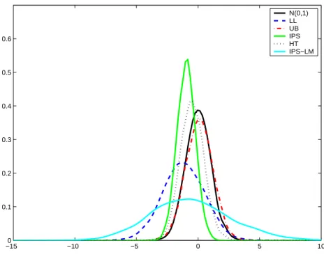
As mentioned already, it is known that for panels of the size available in this study (with T only equal to 13), the asymptotic distributions of panel unit root and panel cointegration tests provide poor approximations to the small sample distributions (see e.g. Hlouskova and Wagner, 2006a). Hence, the notorious size and power problems for which unit root tests are known in the time series context also appear in short panels. In Figure 1 we display the asymptotic null distribution (the standard normal distribution) and the bootstrap null distributions (from the non-parametric bootstrap) when testing for a unit root in CO

emis- sions including only fixed effects in the test specification, for the five asymptotically standard normally distributed tests. The figure shows substantial differences between the bootstrap approximations to the finite sample distribution of the tests and their asymptotic distribu- tion. Thus, basing inference on the asymptotic critical values can lead to substantial size distortions. The discrepancy between the asymptotic and the bootstrap critical values can also be seen in Table 1, where the 5% bootstrap critical values are displayed in brackets. They vary substantially both across tests and also across the two variables. In most cases they are far away from the asymptotic critical values ± 1 . 645, respectively 249 . 128 for the Maddala and Wu test.

It is customary practice in unit root testing to test in specifications with and without linear trends included. A linear trend in the test equation, when there is no trend in the data generating process reduces the power of the tests. Conversely, omitting a trend when there is a trend in the data, induces a bias in the tests towards the null hypothesis. Graphical inspection

14By appropriate scaling and forN → ∞, Choi (2001) derives asymptotically standard normally distributed tests based on this idea.

−150 −10 −5 0 5 10 0.1

0.2 0.3 0.4 0.5 0.6

N(0,1) LL UB IPS HT IPS−LM

Figure 1: Bootstrap test statistic distributions for CO

for 5 asymptotically standard normally distributed panel unit root tests.

The results are based on the non-parametric bootstrap with 5000 replications. Fixed effects are included.

of the data leads us to conclude that for CO

emissions the specification without trend might be sufficient, whereas for GDP the specification with trend might be more appropriate. The nature of the trend component of GDP is a widely discussed topic in macro-econometrics.

Both, unit root nonstationarity with its underlying stochastic trend or trend-stationarity

with usually a linear deterministic trend are plausible and widely used specifications. This

uncertainty concerning the trend specification for GDP manifests itself also in our panel test

results, see below. For completeness we report both types of results for both variables. The

first block in Table 1 displays the results for the parametric bootstrap, the second for the

non-parametric bootstrap and the third for the RBB bootstrap. Within each of the blocks,

the first block-row shows the results with fixed effects and the second the results when both

fixed effects and linear trends are included.

P A RAMETRIC BOOTSTRAP Va ri a b le LL U B IP S H T IP S − LM M W Fixed Effects CO

-2.807* (-3.957) 0.915 (-2.159) 0.229 (-1.707) -4.828* (-5.705) -1.291 (1.096) 310.781* (313.176) GDP -5.890 (-3.197) 1.512 (-2.626) -1.590 (-0.582) 4.321 (3.216) 0.070 (1.231) 422.513 (329.209) Fixed Effects a nd T rends CO

-8.493 (-6.501) -0.565 (-1.121) -2.093 (-1.823) -8.618 (-12.711) 0.259 (0.276) 418.543 (362.505) GDP -15.911 (-2.635) 2.072 (-1.167) -3.423 (-1.346) 12.302 (4.419) 0.456 (0.301) 530.792 (378.350) NON-P A RAMETRIC BOOTSTRAP LL U B IP S H T IP S − LM M W Fixed Effects CO

-2.807 (-2.023) 0.915 (-4.166) 0.230 (-1.628) -4.828 (-1.029) -1.291 (-1.343) 310.781 (309.904) GDP -5.890 (-1.775) 1.512 (-0.974) -1.590 (2.070) 4.321 (5.241) 0.070 (0.361) 422.515 (323.413) Fixed Effects a nd T rends CO

-8.493* (-10.289) -0.565 (-1.226) -2.094* (-2.485) -8.618* (-12.774) 0.259 (0.182) 418.543 (403.105) GDP -15.911 (-8.711) 2.072 (-1.176) -3.423 (-1.789) 12.302 (13.777) 0.456 (0.201) 530.792 (409.514) RESIDUAL BASED B LOCK BOOTSTRAP LL U B IP S H T IP S − LM M W Fixed Effects CO

-2.807* (-7.603) 0.915 (-5.999) 0.230 (-4.094) -4.828* (-8.351) -1.291 (3.006) 310.781* (364.274) GDP -5.890* (-9.082) 1.512 (-6.344) -1.590 (-4.896) 4.321 (-6.901) 0.070 (3.846) 422.513 (392.093) Fixed Effects a nd T rends CO

-8.493* (-23.999) -0.565 (-1.222) -2.094 (-6.096) -8.618 (-8.462) 0.259 (4.226) 418.543* (608.021) GDP -15.911* (-18.717) 2.072 (-2.120) -3.423* (-8.631) 12.302 (-5.887) 0.456 (4.694) 530.792* (663.504) T a ble 1 : R esults of first generation panel unit ro o t tests for the logarithm of p er capita C O

emissions a nd the logarithm of p er capita GDP including only fixed effects in the upp er blo ck-ro ws and fi xed effects a nd linear trends in the lo w er b lo ck -ro w s. The first part of the table corresp o nds to the parametric b o otstrap, the second to the non-parametric b o otstrap a nd the third to the residual b ased blo ck b o o tstrap. In p aren theses the 5 % critical v alues o btained b y the three differen t b o o tstrap metho ds are d ispla y ed. The asymptotic 5 % critical v alue is giv en b y -1.645 for the first 4 tests, b y 1 .645 for IPS-LM a nd b y 249.128 for M W. Bold indicates rejection o f the n u ll h y p o thesis b ased on the b o otstrap critical v alues a nd bo ld * indicates rejection based u p o n the asymptotic critical v alues but no rejection a ccording to the b o otstrap critical v alues. The autoregressiv e lag lengths in b o th the autoregression based tests, in the parametric b o otstrap a nd the non-parametric b o otstrap are equal to 1. The blo ck-length in the RBB b o o tstrap is equal to 2.

Let us start with (the logarithm of per capita) CO

emissions. For all three bootstrap methods and for the majority of tests the null hypothesis of a unit root is not rejected. Only for the parametric bootstrap and the specification with intercepts and trends, and for the non-parametric bootstrap with intercepts the unit root hypothesis is rejected for three of the six tests. In the latter case the rejection of the null with the MW test is a borderline case with a test statistic of 310.781 and a bootstrap critical value of 309.904. Importantly, in the specification with only intercepts, the parametric and the RBB bootstrap lead to non-rejection of the unit root hypothesis for all six tests. A further important observation is that these two bootstraps indicate incorrect rejection of the null for three of the six tests when inference is based on the asymptotic critical values. This exemplifies again the potential pitfalls of using asymptotic critical values for the short panel at hand. Summing up, there is some evidence for unit root nonstationarity of CO

emissions, when using first generation panel unit root tests. Note, however, that by choosing the ‘appropriate’ test and by using the asymptotic critical values the rejection of the unit root null hypothesis can be ‘achieved’.

We now turn to (the logarithm of real per capita) GDP. Starting with the specification including trends we see that three (parametric), two (non-parametric) and six (RBB) tests do not reject the null hypothesis of a unit root when the bootstrap critical values are used. Based on the RBB bootstrap the test decisions differ for three tests when based on the asymptotic critical values and when based on the bootstrap critical values. Thus, quite surprisingly more than for CO

emissions, the unit root tests lead to an unclear picture for per capita GDP.

The same ambiguity prevails when including only fixed effects in the tests. Again, depending upon the choice of unit root test, bootstrap or asymptotic critical values, evidence for unit root stationarity or trend stationarity can be ‘generated’ by first generation panel unit root tests.

3.2 Second Generation Tests

In this subsection we now discuss the results obtained with several second generation panel unit root tests that allow for cross-sectional correlation.

Since there is no natural ordering in the cross-sectional dimension as compared to the time dimension, the first issue is to find tractable specifications of models for cross-sectional dependence in non-stationary panels.

15We do not report bootstrap inference on these second generation methods. To our knowledge an analysis of the small sample performance of these tests is still lacking. The construction of consistent bootstrap methods for cross-sectionally correlated nonstationary panels is furthermore itself an interesting question.

There are two main strands that have been followed in the literature, one is a factor model approach, the other is based – more classical for the panel literature – on error components models.

Let us turn to the idea of the factor model approach first. In this set-up the cross-sectional correlation is due to common factors that are loaded in all the individual country variables, e.g.

x

= ρ

x

+ λ

F

+ u

(4) Here F

∈ R

are the common factors and λ

∈ R

are the so called factor loadings. In general the factors can be either stationary or integrated. After de-factoring the data, i.e.

subtracting the factor component contained in the variables in each country, panel unit root tests (of the first generation type) can be applied to the asymptotically cross-sectionally uncorrelated de-factored data.

The most general approach in this spirit is due to Bai and Ng (2004). They provide estimation criteria for the number of factors, as well as – in the case of more than one common factor – tests for the number of common trends in the factors.

Thus, the factors are allowed to be stationary or integrated of order 1. After subtracting the estimated factor component, Bai and Ng (2004) propose Fisher type panel unit root tests in the spirit of Maddala and Wu (1999) and Choi (2001). The first one is asymptotically χ

distributed, BN

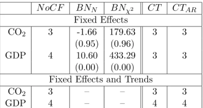
and the second is asymptotically standard normally distributed, BN

. The two tests are specified against the heterogeneous alternative. See the results in Table 2. The number of common factors is estimated to be three for CO

and four for GDP. These estimation results are based on the information criterion BIC

, see Bai and Ng (2004) for details. The two tests for common trends within the common factors, CT and CT

, result in three common trends, except for GDP when both fixed effects and individual trends are included (where four common trends are found).

Thus, essentially all common factors seem to be nonstationary.

Let us next turn to the unit root tests on the de-factored data (only implemented for the fixed effects specification). Somewhat surprisingly the null hypothesis is not rejected for CO

emissions, but is clearly rejected for GDP by both tests. Thus, it seems that some nonstationary idiosyncratic component is present in the CO

emissions series.

16Testing for common trends can be seen as the multivariate analogue to testing for unit roots. In case of a single common factor, a unit root test for this common factor is sufficient, of course.

17The two tests for the number of common trends differ in the treatment of serial correlation. In CT a non-parametric correction is performed, whereasCTARis based on a vector autoregressive model fitted to the

NoCF BN

BN

CT CT

Fixed Effects

CO

3 -1.66 179.63 3 3

(0.95) (0.96)

GDP 4 10.60 433.29 3 3

(0.00) (0.00) Fixed Effects and Trends

CO

3 – – 3 3

GDP 4 – – 4 4

Table 2: Results of Bai and Ng (2004) PANIC analysis. NoCF indicates the estimated number of common factors according to BIC

. BN

and BN

denote the unit root tests on the de-factored data. CT and CT

denote the estimated number of common trends within the common factors.

The p –values are displayed in brackets, with 0.00 indicating p –values smaller than 0.005.

Bai and Ng (2004) present the most general factor model approach to non-stationary panels currently available and the only one that allows for testing also the stochastic properties of the common factors. For completeness we also report the results obtained with two more restricted factor model approaches, due to Moon and Perron (2004) and Pesaran (2003). Moon and Perron (2004) present pooled t -type test statistics based on de-factored data (where we use the factors estimated according to Bai and Ng). We report two asymptotically standard normally distributed tests with serial correlation correction in the spirit of Phillips and Perron (1988), denoted with MP

and MP

. Pesaran (2003) provides an extension of the Im, Pesaran, and Shin (2003) test to allow for one factor with heterogeneous loadings. His procedure, which is a suitably cross-sectionally augmented IPS Dickey Fuller type test, works by including cross- section averages of the level and of lagged differences to the IPS-type regression. Pesaran (2003) considers two versions: the procedure just described, denoted with C − IP S and a truncated, robust version C − IP S

. For both of his tests the distribution is non-standard and has to be obtained by simulation methods.

The results from these factor model approaches are contained in the upper block of Table 3.

The null hypothesis of a unit root is rejected in all cases (at least when testing at 6%) except for CO

when individual specific trends are included. Thus, all factor based unit root tests reject the unit root null hypothesis on de-factored GDP. This seems to indicate that there are global common stochastic factors (respectively trends, compare the results obtained with the

common factors.

Fixed Effects Fixed Effects & Trends

CO

GDP CO

GDP

MP

-22.70 -17.00 -7.79 -11.58 (0.00) (0.00) (0.00) (0.00) MP

-13.33 -15.70 -14.71 -27.63 (0.00) (0.00) (0.00) (0.00) C − IP S -2.09 -2.12 -1.83 -2.76

(0.06) (0.05) (0.95) (0.04) C − IP S

-2.08 -2.11 -1.83 -2.74

(0.06) (0.05) (0.95) (0.04)

C

9.62 5.80 6.94 2.97

(0.00) (0.00) (0.00) (0.00)

C

-8.98 -6.46 -6.79 -3.87

(0.00) (0.00) (0.00) (0.00)

C

-9.06 -6.15 -6.95 -3.82

(0.00) (0.00) (0.00) (0.00) NL − IV

1.84 12.79 -0.24 -1.01

(0.97) (1.00) (0.41) (0.16)

NL − IV

8.43 13.43 0.21 -0.71

(1.00) (1.00) (0.58) (0.24)

NL − IV

3.84 11.64 0.99 1.47

(1.00) (1.00) (0.84) (0.93)

Table 3: Results of second generation panel unit root tests. The left block-column contains the results when only fixed effects are included. The right block-column contains the results when both fixed effects and individual specific linear trends are included.

In brackets the p –values are displayed, with 0.00 indicating p –values smaller than 0.005.

Bai and Ng methodology) in the GDP country data for our 107 countries. Note again that the results obtained by applying the Moon and Perron test and the Pesaran test are strictly speaking only valid if there is only one factor. For our very short panel, it may however be appropriate to compare the results obtained by several methods.

Choi (2006) presents test statistics based on an error component model. His tests are based on eliminating both the deterministic components and the cross-sectional correlations by applying cross-sectional demeaning and GLS de-trending to the data.

Based on these preliminary steps Choi proposes three group-mean tests based on the Fisher test principle, which differ in scaling and aggregation of the p -values of the individual tests. All three test statistics, C

, C

and C

, are asymptotically standard normally distributed. The individ-

18This model structure can, equivalently, be interpreted as a factor model with one factor and identical loadings for all units.

ual test underlying the implementation of this idea in the present study is the augmented Dickey-Fuller test. The results are quite clear: The null hypothesis of a unit root is rejected throughout variables and specifications.

Finally, Chang (2002) presents panel unit root tests that handle cross-sectional correlation by applying nonlinear instrumental variable estimation of the (usual) individual augmented Dickey-Fuller regressions. The instruments are given by integrable functions of the lagged levels of the variable and the test statistic is given by the standardized sum of the individual t -statistics. We present the results for three different instrument generating functions, termed NL− IV

for i = 1 , 2 , 3. The results are completely different from the other second generation panel unit root test results: The null hypothesis of a unit root is not rejected by any of the three tests for both variables and both specifications of the deterministic components. The difference in results may be explained by the Im and Pesaran (2003) comment on the Chang nonlinear IV tests. Im and Pesaran (2003) show that the asymptotic behavior established in Chang (2002) holds only for N ln T/ √

T → 0, which requires N being very small compared to T . This is of course not the case in our data set with N = 107 countries and T = 13 years.

Thus, the results of the Chang NL-IV tests should be interpreted very carefully.

3.3 Conclusions from Panel Unit Root Analysis

There seems to be evidence for cross-sectional correlation for both variables. The results obtained with the method of Bai and Ng (2004) indicate the presence of three to four inte- grated common factors. The general conclusion from the second generation tests, except for the Chang tests, is that after subtracting the common factors, the idiosyncratic components may well be stationary. The evidence in that direction is stronger for GDP than for CO

emissions.

The evidence for cross-sectional correlation fundamentally weakens the basis of the results

obtained by applying first generation tests. Thus, for these tests we only want to highlight

again the main conclusions that can be made even without resorting to second generation

methods. First, the bootstrap test distributions differ substantially from the asymptotic

test distributions. This implies that test results based on bootstrap critical values can often

differ from test results based on asymptotic critical values. Second, by choosing the unit

root test and/or the bootstrap strategically any conclusion can be ‘supported’. This large

uncertainty around the results should urge researchers to be much more cautious than usual

in the empirical EKC literature.

4 Panel Cointegration Tests

In this section we present panel cointegration tests for cross-sectionally uncorrelated panels.

We do this to show, similarly to the panel unit root tests, that a more careful application of these methods would lead researchers to be skeptical about the validity of their results. This second level discussion is, of course overshadowed by the two first level problems.

We test for the null of no cointegration in both the linear (2) and the quadratic (1) specification of the relationship between the logarithm of per capita CO

emissions and the logarithm of per capita GDP. We test in quadratic version solely to show that a careful statistical analysis with the available (but inappropriate) tools of panel cointegration would already lead to ambiguous results. In particular we show that the test results depend highly upon the test applied and whether the asymptotic or some bootstrap critical values are chosen. These observations, which can be made by just using standard methods, should lead the researcher to draw only very cautious conclusions. Of course, we know from the discussion in Section 2 that cointegration in the usual sense is not defined in equation (1).

This observation has been ignored in the empirical literature and several published papers, e.g., Perman and Stern (2003) discuss ‘cointegration’ in the quadratic specification based on unit root testing for emissions, GDP and the square of GDP.

We have in total performed ten cointegration tests, seven of them developed in Pedroni (2004) and three in Kao (1999). Similar bootstrap procedures as for the panel unit root tests are applied, see the description in Appendix B. The results obtained by applying the three tests developed by Kao are not displayed but are available from the authors upon request in a separate appendix.

All tests are formulated for the null hypothesis of no cointegration, see Hlouskova and Wagner (2006b) for a discussion and a simulation based performance analysis including all

19Kao (1999) derives tests similar to three of the pooled tests of Pedroni for homogenouspanels when only fixed effects are included. A panel is called homogenous, if the serial correlation pattern is identical across units. Kao’s three tests,Kρ,Kt and Kdf, are based on the spurious least squares dummy variable (LSDV) estimator of the cointegrating regression. We have also performed these tests, since tests based on a cross- sectional homogeneity assumption might perform comparatively well even when the serial correlation patterns differ across units. This may be so, because no individual specific correlation corrections, that may be very inaccurate in short panels, have to be performed. Kao’s tests are after scaling and centering appropriately asymptotically standard normally distributed and left sided. The results are qualitatively similar to the results obtained with Pedroni’s tests.

the panel cointegration tests used in this paper. The tests are based on the residuals of the so called cointegrating regression, in our example in the linear case given by (2):

ln( e

) = α

+ γ

t + β

ln ( y

) + u

If both log emissions and log GDP are integrated, the possibility for cointegration between the two variables arises. Cointegration means that there exists a linear combination of the vari- ables that is stationary. Thus, the null hypothesis of no cointegration in the above equation is equivalent to the hypothesis of a unit root in the residuals, ˆ u

say, of the cointegrating re- gression. The usual specifications concerning deterministic variables have been implemented.

In Table 4 we report test results when including only fixed effects and when including fixed effects and individual specific trends.

Pedroni (2004) develops four pooled tests and three group-mean tests. Three of the four pooled tests are based on a first order autoregression and correction factors in the spirit of Phillips and Ouliaris (1990). These are a variance-ratio statistic, P P

; a test statistic based on the estimated first-order correlation coefficient, P P

; and a test based on the t -value of the correlation coefficient, P P

. The fourth test is based on an augmented Dickey-Fuller type test statistic, P P

, in which the correction for serial correlation is achieved by augmenting the test equation by lagged differenced residuals of the cointegrating regression. Thus, this test is a panel cointegration analogue of the panel unit root test of Levin, Lin, and Chu (2002).

For these four tests the alternative hypothesis is stationarity with a homogeneity restriction on the first order correlation in all cross-section units.

To allow for a slightly less restrictive alternative, Pedroni (2004) develops three group- mean tests. For these tests the alternative allows for completely heterogeneous correlation patterns in the different cross-section members. Pedroni discusses the group-mean analogues of all but the variance-ratio test statistic. Similarly to the pooled tests, we denote them with P G

, P G

and P G

. We report both the pooled and group-mean test results to see whether the test behavior differs systematically between these two types of tests.

After centering and scaling the test statistics by suitable correction factors, to correct for serial correlation of the residuals and for potential endogeneity of the regressors in the cointegrating regression, all test statistics are asymptotically standard normally distributed.

20For such a short panel as given here, systems based methods like the one developed in Groen and Kleibergen (2003) are not applicable.

Figures similar to Figure 1 are available from the authors upon request. Again substantial differences between the asymptotic critical values and the bootstrap critical values emerge.

The first block in Table 4 corresponds to the parametric bootstrap, the second to the non-parametric bootstrap and the third to the RBB bootstrap. Within each block, the first block-row corresponds to the linear specification and the second to the quadratic specification.

Both, the linear and the quadratic specification have been tested with fixed effects and with fixed effects and individual specific linear trends. Just to be sure, note again, that testing for cointegration in the quadratic formulation lacks theoretical econometric foundations.

Let us start with the linear specification, which is ‘only’ subject to the first level problem of cross-sectional correlation. There is some variability of results across bootstrap methods and again in a variety of cases bootstrap inference leads to different conclusions than resorting to the asymptotic critical values. This happens in particular for the RBB bootstrap. For the quadratic specification, i.e. the Kuznets curve in its usual formulation, roughly the same observations as for the linear specification can be made, ignoring again the problem that a correct econometric foundation is lacking due to the nonlinear transformation. Again the RBB bootstrap leads to the fewest rejections of the null hypothesis. The null hypothesis of no cointegration is more often rejected for the linear formulation than for the quadratic specification. Note that no systematic differences between the pooled and the group-mean tests occur.

The above results provide some weak evidence for the presence of a cointegrating rela- tionship between GDP and emissions. However, as for the panel unit root tests, by choosing the test and the bootstrap strategically, any ‘conclusion’ can be supported. This ‘volatility’

of the results should lead researchers to be more cautious than what is usually observed.

P A RAMETRIC BOOTSTRAP PP

PP

PP

PP

PG

PG

PG

Linear Sp ecification FE 2.887* (3.670) -3.121 (-3.129) -7.061 (-6.501) -4.899 (-0.041) -1.595 (-0.041) -10.498 (-6.569) -10.956 (-6.949) FE & T r. 1.155 (1.484) -3.045 (-0.872) -14.877 (-9.721) -12.827 (-7.840) 1.477 (3.002) -13.058 (-8.046) -14.352 (-9.149) Quadratic S p ecification FE 0.434 (2.761) -0.382 (-1.197) -6.528* (-7.827) -4.769* (-6.173) 2.335 (2.401) -8.766 (-8.035) -9.718 (-8.927) FE & T r. -0.954 (-0.457) 0.639 (2.174) -14.454 (-9.529) -11.985 (-7.456) 4.592 (5.611) -13.325 (-9.386) -14.596 (-10.554) NON-P A RAMETRIC BOOTSTRAP PP

PP

PP

PP

PG

PG

PG

Linear Sp ecification FE 2.887 (0.858) -3.121 (-1.880) -7.061 (-5.261) -4.899 (-3.593) -1.595 (0.364) -10.498 (-6.124) -10.956 (-6.424) FE & T r. 1.155 (1.498) -3.045 (-0.814) -14.877 (-9.582) -12.827 (-7.772) 1.477 (3.027) -13.058 (-7.873) -14.352 (-9.018) Quadratic S p ecification FE 0.434 (1.023) -0.382 (-0.792) -6.528* (-7.193) -4.769* (-5.574) 2.336 (2.647) -8.766 (-7.552) -9.718 (-8.405) FE & T r. -0.953 (-0.413) 0.639 (2.160) -14.454 (-9.429) -11.985 (-7.432) 4.592 (5.586) -13.325 (-9.331) -14.596 (-10.562) RESIDUAL BASED B LOCK BOOTSTRAP PP

PP

PP

PP

PG

PG

PG

Linear Sp ecification FE 2.887* (3.089) -3.121 (-2.947) -7.061 (-6.933) -4.899* (-5.269) -1.595 (-0.915) -10.498 (-9.134) -10.956 (-9.777) FE & T r. 1.155 (2.947) -3.045* (-3.296) -14.877 (-15.231) -12.827 (-12.725) 1.477 (0.936) -13.058* (-14.977) -14.352* (-16.341) Quadratic S p ecification FE 0.434 (0.975) -0.382 (-1.274) -6.528* (-8.733) -4.769* (-7.016) 2.336 (1.085) -8.766* (-12.976) -9.718* (-14.153) FE & T r. -0.936 (0.503) 0.639 (0.0490) -14.454 (-15.303) -11.985* (-12.150) 4.592 (3.604) -13.325* (-17.100) -14.596* (-19.070) T a ble 4 : R esults of P edroni’s panel coin tegration tests including fixed effects o nly (FE), resp ectiv ely fi xed effects and linear trends (FE & T r.). The upp er blo ck-ro w d ispla y s the results for the linear sp ecification a nd the lo w er b lo ck -ro w displa ys the results for the quadratic sp ecification. The first part of the table corresp o nds to the parametric b o otstrap, the second to the non-parametric b o otstrap a nd the third to the residual b ased blo ck b o o tstrap. The asymptotic 5 % critical v alue is giv en b y 1 .645 for the first test and b y -1.645 for the other 6 tests. Bold indicates rejection o f the n u ll h y p o thesis b ased on the b o otstrap critical v alues a nd bo ld * indicates rejection based u p o n the asymptotic critical v alues but no rejection a ccording to the b o otstrap critical v alues. The autoregressiv e lag lengths in b o th the autoregression based tests, the parametric b o otstrap a nd the non-parametric b o otstrap a re equal to 1. The windo w-length of the Bartlett k ernels u sed in the non-parametric tests is a lso equal to 1. The blo ck-length in the RBB b o o tstrap is equal to 2.

5 Estimation of the Carbon Kuznets Curve with Panel Coin- tegration Methods and Using De-factored Observations

We finally turn to estimating the CKC relationship. In the first subsection we estimate the CKC with panel cointegration methods that correspond to the first generation panel unit root and cointegration tests. These methods are of course subject to the two first level critiques. As for the panel unit root and cointegration tests, we include results based on this type of methods to show that by careful application the conclusions one could draw, even when staying in this framework, are very weak. In the second subsection we estimate the CKC relationship on de-factored data. These are, up to potentially bad small sample performance of the Bai and Ng (2004) procedure, stationary. Thus, for these data standard panel regression techniques are applicable. Note also that the de-factored data are (asymptotically) cross-sectionally uncorrelated.

5.1 Panel Cointegration Estimation

Two types of estimators for the cointegrating relationship in panels are applied: fully mod-

ified ordinary least squares (FM-OLS) and dynamic ordinary least squares (D-OLS). Both

estimation methods are panel extensions of well known time series concepts. FM-OLS was

introduced by Phillips and Hansen (1990) and D-OLS is due to Saikkonen (1991). Both meth-

ods allow for serial correlation in the residuals and for endogeneity of the regressors in the

cointegrating regression. The panel extensions of FM-OLS are discussed in detail in Phillips

and Moon (1999), nesting the discussions in Pedroni (2000) and Kao and Chiang (2000). As

in the time series case, the idea of FM-OLS is to obtain in the first step OLS estimates of

long-run variance matrices. In the second step another regression is run on corrected variables,

with the correction factors being functions of the estimated long-run variance matrices. The

idea of D-OLS is to correct for serial correlation and endogeneity by augmenting the cointe-

grating regression by leads and lags of first differences of the regressors. The panel extensions

of D-OLS are discussed in Kao and Chiang (2000) and Mark and Sul (2003). Both methods,

FM-OLS and D-OLS, yield asymptotically normally distributed (for first T followed by N to

infinity) estimated cointegrating vectors, which implies that χ

inference via e.g. Wald tests

can be conducted. Note for completeness that various versions of both FM-OLS and D-OLS in

weighted or unweighted fashions have been implemented, see Hlouskova and Wagner (2006b)

for a description. These differ i.a. in how the correction factors are computed.