BANKRUPTCY PREDICTIONS AND TEXTUAL ANALYSIS OF EARNINGS FORECASTS , T HREE ESSAYS ON THE PERFORMANCE

OF EARNINGS FORECASTS ,

BANKRUPTCY PREDICTIONS AND TEXTUAL ANALYSIS

I n a u g u r a l d i s s e r t a t i o n z u r

E r l a n g u n g d e s D o k t o r g r a d e s d e r

W i r t s c h a f t s - u n d S o z i a l w i s s e n s c h a f t l i c h e n F a k u l t ä t d e r

U n i v e r s i t ä t z u K ö l n 2 0 1 9

v o r g e l e g t v o n

T o b i a s L o r s b a c h , M . S c . a u s

P r ü m

Vorsitz: Univ.-Prof. Dr. Thomas Hartmann-Wendels

Tag der Promotion: 06. Juni 2019

This thesis consists of the following works:

Hess, Dieter and Tobias Lorsbach (2019):

Incorporating Quarterly Earnings Information into Cross-Sectional Earnings Forecast Models,

Working Paper, University of Cologne.

Huettemann, Martin and Tobias Lorsbach (2019):

The Quality of Bankruptcy Data and its Impact on the Evaluation of Prediction Models:

Creating and Testing a German Database, Working Paper, University of Cologne.

Lorsbach, Tobias (2019):

Word Power: Content Analysis in the Presence of Competing Information,

Working Paper, University of Cologne.

Die vorliegende Arbeit habe ich während meiner Zeit als Promotionsstudent der Cologne Graduate School in Management, Economics and Social Sciences und Wissenschaftlicher Mitarbeiter am Lehrstuhl für ABWL und Unternehmensfinanzen an der Universität zu Köln angefertigt.

In erster Linie möchte ich mich bei meinem Doktorvater Prof. Dr. Dieter Hess für die umfassende Betreuung meiner Arbeit in den vergangenen vier Jahren bedanken.

Ich bedanke mich auch bei Prof. Dr. Alexander Kempf für die Erstellung des Zweitgutachtens, sowie Prof. Dr. Thomas Hartmann-Wendels für die Übernahme des Vorsitzes der Prüfungskommission.

Weiterhin bedanke ich mich bei der Cologne Graduate School in Management.

Economics and Social Sciences für die umfangreiche Förderung, sowie insbesondere ihrer Direktorin Dr. Dagmar Weiler für die anhaltende administrative und auch persönliche Unterstützung im Rahmen meines Promotionsstipendiums.

Insbesondere bedanke ich mich bei Martin Hüttemann für die tolle Zusammenarbeit bei dem gemeinsamen Forschungsprojekt, sowie William Liu für die zahlreichen Diskussionen und Kommentare. Außerdem bedanke ich mich bei meinen weiteren Kollegen an der Cologne Graduate School und dem Lehrstuhl für ABWL und Unternehmensfinanzen an der Universität zu Köln: Niklas Blümke, Anke Gewand, Martin Meuter, Britta Plum, Tim Vater und Djarban Waning.

Zu guter Letzt, möchte ich mich herzlich bei meinem privaten Umfeld, Freunden und Familie, bedanken. Insbesondere bedanke ich mich bei meinen Eltern, sowie meinen beiden Geschwistern für die gesamte Unterstützung und Zuspruch während der Promotion, aber auch allen anderen bisherigen Lebensphasen und -situationen.

Tobias Lorsbach

I

Page List of Figures ... III List of Tables ... IV

1 Introduction ... 1

2 Incorporating Quarterly Earnings Information into Cross-Sectional Earnings Forecast Models ... 10

2.1 Introduction ... 10

2.2 Model development ... 16

2.3 Methods and data ... 22

2.4 Empirical results ... 26

2.5 Conclusion ... 47

3 The Quality of Bankruptcy Data and its Impact on the Evaluation of Prediction Models: Creating and Testing a German Database ... 49

3.1 Introduction ... 49

3.2 Our bankruptcy database ... 53

3.3 Data and method ... 65

3.4 Empirical results ... 68

3.5 Conclusion ... 79

II

4 Word Power: Tone Analysis in the Presence of Competing Information ... 80

4.1 Introduction ... 80

4.2 Approach of content analysis ... 84

4.3 Theoretical framework and hypothesis development ... 86

4.4 Data and implementation ... 91

4.5 Empirical results ... 94

4.6 Conclusion and future research ... 107

Bibliography ... 109

Appendices ... 119

III

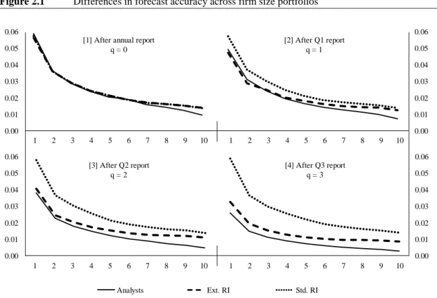
Page Figure 2.1 Differences in forecast accuracy across firm size portfolios ... 38

Figure 4.1 Bayesian learning from earnings announcements (EAD)

and 10-K filings (FIL) ... 86 Figure 4.2 Timing of 10-K filings (FIL)

and earnings announcement dates (EAD) ... 96

Figure 4.3 Sensitivity of word strengths from year to year ... 103

IV

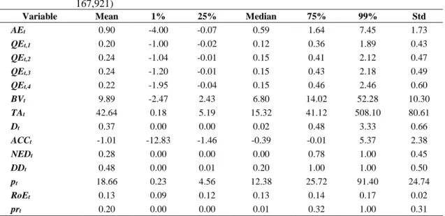
Page Table 2.1 Descriptive sample statistics of cross-sectional regression

Variables, 1982-2014 (N = 167,921) ... 25

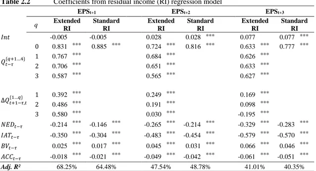
Table 2.2 Coefficients from residual income (RI) regression model ... 26

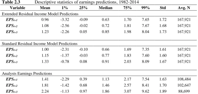
Table 2.3 Descriptive statistics of earnings predictions, 1982-2014 ... 28

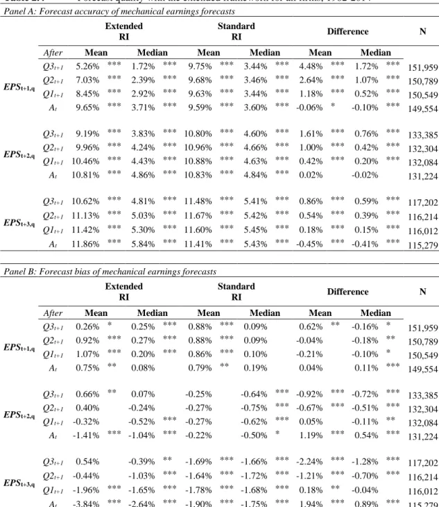
Table 2.4 Forecast quality with the extended framework for all firms, 1982-2014 ... 30

Table 2.5 Relation between model-based forecast accuracy (EPS

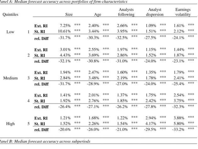
) and firm characteristics, subperiods and subsamples ... 32

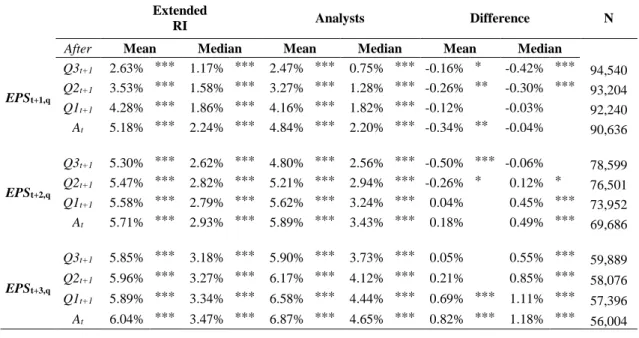
Table 2.6 Comparison of model’s forecast accuracy against professional equity analysts ... 36

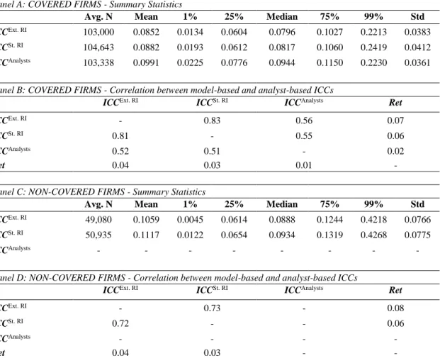
Table 2.7 Descriptive statistics of composite ICC estimates, 1982-2014 ... 40

Table 2.8 Portfolio strategies on ICC estimates ... 42

Table 2.9 Firm-level regressions of returns and ICCs... 46

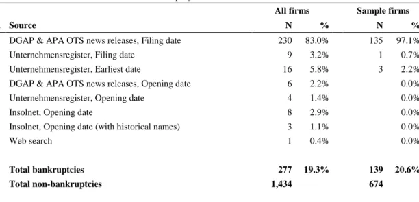
Table 3.1 Data sources of HL bankruptcy data ... 58

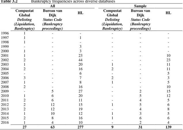
Table 3.2 Bankruptcy frequencies across diverse databases ... 59

Table 3.3 Bankruptcy frequencies across databases (not covered in HL)... 61

Table 3.4 Largest bankruptcies covered in diverse databases ... 62

Table 3.5 Differences in bankruptcy dates across HL, Compustat and Bureau van Dijk data ... 63

Table 3.6 Summary statistics of variables within selected bankruptcy models (N = 95,431) ... 66

Table 3.7 Parameter estimates of common bankruptcy models ... 69

Table 3.8 Out-of-sample results: Comparison across models ... 71

Table 3.9 Parameter estimates of bankruptcy models using sample ranges covered in Bureau van Dijk (N = 24,457) ... 73

Table 3.10 Out-of-sample results: Comparison across bankruptcy databases ... 76

V

Table 4.1 Sample construction ... 92

Table 4.2 Sample summary statistics ... 95

Table 4.3 Univariate analysis – Market reactions to competing information ... 98

Table 4.4 Multivariate analysis – Market reactions to competing information ... 99

Table 4.5 Tone measure based on earnings announcement (EADRet) and filing returns (FILRet) ... 101

Table 4.6 Comparison of word power weights across different models ... 102

Table 4.7 Textual tone and future performance ... 105

1

Chapter 1 Introduction

In efficient capital markets, market prices reflect all available information.

Market participants receive most of their financial information by annual and quarterly reports, that are the official statements of a company’s profitability. By this, they include all information on company business operations and conditions, potential risks, litigation, profits, and current financial health. The information provided can be quantitative and qualitative in nature. Quantitative information is presented in graphs, tables, and most importantly, numbers and can be assessed easily because of its nature. The analysis of such information is a central theme in finance and capital markets research in accounting.

For example, earnings figures and growth rates have been frequently used as fundamental inputs in several corporate finance settings, such as firm valuation or capital budgeting.

Moreover, they take a crucial part to investment management practices of fund managers and investors. In contrast, qualitative information refers to unstructured data that is presented as written and spoken text and that is not readily quantified by numbers. In turn, an emerging discipline of science develops methods of content analyses to measure components, such as sentiment and readability, of textual data (see, e.g., Henry, 2008;

Loughran and McDonald, 2011) that is typically interpreted by cognitive processing of

each individual. However, human cognitive capabilities are limited, and, thus, financial

2

intermediaries play a central role in collecting, processing and analyzing material data from corporate disclosures to provide capital markets with aggregated information.

Traditionally, auditors, financial analysts, and rating agencies have been the most important specialized information intermediaries in financial markets. Due to their reputation and regulations stakeholders used to have confidence in information provided by these intermediaries. However, recently, investor confidence evaporates because renowned auditors were involved in numerous accounting scandals and because rating agencies biased their appraisals in favor of issuer clients during the financial crisis. In addition, company analyses made by financial analysts appear to be substantially off-the- mark and forecasts are notoriously biased toward optimistic prospectuses (see, e.g., Abarbanell, 1991; O’Brien, 1988; Bradshaw et al., 2012). Therefore, in course of the digital revolution, company stakeholders, including investors, banks, regulators, and the media, have devoted significant resources to substitute major processes of financial intermediaries through technological alternatives. This includes, for example, fully automated investment advisory services using sophisticated computer algorithms, i.e., robo-advisers, sharing investments in social trading networks or raising funds through crowdfunding platforms. Besides these activities, from an investor’s perspective, company analyses may also substantially benefit from fully automated analyses of quantitative data, such as the automation of the processes of forecasting firm-level earnings, financial insolvencies and liquidity ratings, or the creation of computerized analyses of qualitative content from company financial reports.

In Chapter 1 of my thesis, which is based on “Incorporating Quarterly Earnings

information into Cross-Sectional Earnings Forecast Models” (2019) and is co-authored

by Dieter Hess, I address this several aspects of this issue. In this article, we develop a

novel framework to automatically update earnings forecast models in response to

quarterly earnings results. This allows models’ forecasts to be more informative and at

the same time to provide high-frequency earnings expectations. Accordingly, we compare

model forecasts and analyst forecasts and level the playing field between equity analysts

and mechanical models. In addition, we evaluate the implied cost of capital (ICCs)

estimates that are based on these forecasts. The ICC is the discount rate that equates a

3

firm’s future cash flows to its current stock price (see, e.g., Gordon and Gordon, 1997;

Easton, 2004).

Most importantly, our analyses focus on four aspects. First, we introduce a new approach to incorporating intra-year information into individual cross-sectional forecast models. That is, we explicitly utilize quarterly earnings results to produce more accurate and timely earnings forecasts. Second, we assess whether model forecasts or analysts’

forecasts perform better. Specifically, we analyze the changes in forecast accuracy throughout the financial year and particularly after structural breaks from quarterly earnings reports. Third, we evaluate ICC estimates that are based on these forecasts. Last, we also explore whether better earnings forecasts yield more reliable ICCs.

To innovate forecast models using fundamental interim earnings information, we develop a novel framework for updating model forecasts immediately after earnings release and incorporating that valuable information. Therefore, we adapt the way analysts anticipate quarterly earnings results. In particular, whenever a company discloses a quarterly earnings number, the forecast task for annual earnings reduces to predicting the results for the remaining fiscal quarters. We adjust forecast models to predict only the remaining unknown portion of the annual earnings results. Finally, we aggregate realized quarterly results and our forecasts for the yet unpublished quarterly results into earnings forecasts for the entire fiscal year. Using this concept, we formulate a parsimonious model that produces annual earnings forecasts throughout the year using a company’s most recent financial statements, in a manner similar to analysts.

Our augmented framework produces substantially better earnings forecasts. That

is, forecast errors of annual earnings forecasts made after the release of first quarter results

are reduced by about 15.2%. Correspondingly, the forecasts made after the second and

third quarters are more accurate by about 30.8% and 50.0%., respectively. Moreover, we

find that once model forecasts and analysts’ forecasts are compared systematically

according to available public information, performance differences diminish. In detail,

analysts’ forecasts are more accurate only for the largest 10% of all firms. Hence, model

forecasts efficiently improve forecast accuracy by using quarterly information. Moreover,

we document that ICCs based on model forecasts better predict future returns than those

constructed with analysts’ forecasts. Despite the high accuracy of analysts’ short-term

4

forecasts, we show that analysts’ forecasts, in general, are very optimistic and grossly inaccurate in long-term horizons. Accordingly, analyst-based ICCs are not significantly related to future returns. However, we still find that better forecasts from the earnings model yield better predictors for future stock returns. In fact, model forecasts that incorporate interim earnings information produces better expected return proxies than the initial model specifications. Hence, better forecast quality yields ceteris paribus (c.p.) better proxies for future returns.

This study most closely relates to the work done by Hou et al. (2012) and Li and Mohanram (2014). We apply our framework of adjusting forecast models according to available quarterly earnings information to the model of Hou et al. (2012), hereafter HVZ, and to the residual income (RI) and earnings persistence (EP) models specified by Li and Mohanram (2014). First, we benchmark our extended models against the initial model to test whether model forecasts improve from quarterly earnings information. In previous studies, analysts’ forecasts anticipated fundamental quarterly information, while initial models incorporate only annual earnings information. Accordingly, there is no study that comprehensively compares the earnings forecast performance of equity analysts with that of cross-sectional forecast models (e.g., Feng, 2014). Thereby, we clarify the confounding effects from previous studies that use analyst forecasts and consider quarterly earnings statements by also incorporating this information into model forecasts.

Our results contribute to the literature on earnings forecasts and future return proxies in several ways. First, we find that earnings forecasts can be potentially automated using cross-sectional models and high frequency data. In addition, we show that more accurate earnings expectations translate into more reliable proxies of future returns.

Finally, our results may motivate researchers to further innovate forecast models to

incorporate additional high-frequency data. Traditionally, mechanical models have

exclusively incorporated financial accounting data. However, our findings suggest that

the performance of model earnings forecasts may further improve from additional

information, such as macroeconomic indicators or stock market data, that also carries

valuable information and help to beat equity analysts even in short-term horizons.

5

While a company’s earnings results are a key input in several asset pricing models, for example to estimate the implied cost of capital (see Chapter 2), they are also a primary indicator of a company’s current and future financial strength. The second essay (Chapter 3) is based on my working paper “The Quality of Bankruptcy Data and its Impact on the Evaluation of Prediction Models: Creating and Testing a German Database” (2019) and is co-authored by Martin Huettemann. In this paper, we apply several bankruptcy prediction models in the context of German companies. While the methodology of bankruptcy predictions and choice of predictor variables that may indicate financial weakness have been intensively addressed in previous studies (see, e.g., Altman, 1968; Ohlson, 1980; Shumway, 2001; Bharath and Shumway, 2008), this article focuses on another central aspect: the primary quality of bankruptcy information. In detail, we explore whether imprecise bankruptcy indicators produce confounding results by comparing different bankruptcy models. For this purpose, we create an alternative database of German bankruptcies by systematically collecting information from public sources, testing differences among existing commercial databases and, finally, examining how bankruptcy prediction models are driven by these divergences.

Existing studies commonly use commercial databases to obtain bankruptcy information. In the U.S., LoPucky, the SDC Platinum Database, Moody’s Default and Recovery Database, Capital IQ, and the Fixed Investment Securities Database (FISD) are examples of such databases. Even though the SDC Platinum Database and Moody’s Default and Recovery Database contain some data on European bankruptcies, there is sparse data available for non-U.S. firms. Similarly, there is little literature that captures the predictability of bankruptcies outside the U.S. (see, e.g., Dahiya and Klapper, 2007;

Altman, Iwanicz-Drozdowska, Laitinen, Suvas, 2017; Tian and Yu, 2017). In spite of this, there is no study that provides guidance on how to obtain bankruptcy data from public services (particularly outside the U.S.). None of the existing studies discuss the underlying data of bankruptcy events and, consequently, how this may drive bankruptcy models to perform differently or whether firm characteristics are connected to higher probabilities of default.

The first contribution of this study is that we generate a dataset of bankruptcy

information using automated web scraping and textual analysis. We develop a systematic

methodology to obtain bankruptcy information from corporate news releases and public

6

sources. In detail, we implemented an automated web-scraper to download all publicly available corporate disclosures from online news archives and, furthermore, we crawled relevant public databases to obtain bankruptcy information for public firms in Germany.

Applying this methodology, we compile a bankruptcy database that is more complete and accurate regarding bankruptcy events and dates than the most frequently used commercial databases, i.e., Bureau van Dijk and Compustat Global. Most importantly, our bankruptcy database, hereafter HL, includes bankruptcies that are not reflected in those databases and, hence, it cannot be reproduced by any combination of these commercial databases.

Furthermore, this article contributes to the voluminous literature on bankruptcy prediction research in several ways. That is, we comprehensively compare of popular bankruptcy prediction models for the German market using our solid bankruptcy information database. We use our bankruptcy data to conduct two empirical analyses.

First, we compare the performance of several bankruptcy prediction models in the context of German firms. Second, we compare our database with Bureau van Dijk data and find that the quality of bankruptcy data significantly affects parameter estimates and the out- of-sample evaluation of bankruptcy prediction models. It is likely that previous studies that used incomplete bankruptcy information provided by Bureau van Dijk or Compustat Global present biased parameters for commonly used bankruptcy prediction models. As a result, the out-of-sample assessment based on these biased parameters may not be informative. In detail, we find that when Bureau van Dijk information is used, the out-of- sample evaluation yields completely different inferences than evaluations using our HL data, i.e., the in-sample tests set to other model specifications and the out-of-sample evaluation recommends another prediction model. This suggests that results of previous studies should be reviewed in light of the relevance of underlying bankruptcy data quality.

This article adds important findings to the existing literature on bankruptcy

predictability. In a case study for the German capital market, we show that the underlying

quality of bankruptcy data fundamentally matters to the integrity of bankruptcy prediction

models. This serves investors and researchers equally. On the one hand, researchers may

extend our web-scraping approach to compile even broader data sets of bankruptcy

events, for example, for non-public firms or roll-outs to other capital markets. In addition,

accurate bankruptcy information is crucial for several other applications, such as,

analyzing systemic risk or credit spreads. Hence, investors, banks, rating agencies, and

7

creditors can better validate their bankruptcy prediction models using our German data and, thus, better quantify default risks in credit contracts or improve liquidity classifications and market participants’ ratings using basic financial statement information from annual earnings reports, such as quantitative earnings, asset and liability numbers.

The information content of earnings reports is generally a focal point for many measurement controversies in accounting and finance (e.g., Beaver, 1968). As an alternative to analyzing quantitative data from corporate disclosures (as discussed in Chapters 2 and 3), a growing body of literature derives a new class of data by analyzing textual content within financial news or corporate disclosures. Therefore, turning from direct processing of quantitative information to analyzing textual content, the third essay (Lorsbach, 2019, “Word Power: Content Analysis in the Presence of Competing Information”) introduces a novel framework for quantifying the qualitative content of financial disclosures according to immediate stock market responses. While most researchers use readily available quantitative information, such as earnings numbers or balance sheet items, today’s vast availability of descriptive information about firms found in corporate disclosures, the financial press, and social media have led to an extensive number of opportunities for qualitative content analysis. In general, qualitative information refers to unstructured data from written and spoken texts that are not readily quantified and are generally analyzed through cognitive processing by individuals.

However, complex algorithms and technological progress have made it feasible to process this voluminous unstructured text data using automated procedures.

Traditionally, financial economics has predominantly used “bag-of-words”

methods, such as dictionary-based classifications, to categorize single words as either positive or negative (see, e.g., Henry, 2008; Li, 2008; Loughran and McDonald, 2011).

In contrast, Jegadeesh and Wu (2013) developed an approach that determines the relative

content of words using investors’ cognitive language processing by gauging market

reactions to 10-K filings. However, several studies find that investor responses to 10-K

filings are not significant per se and are essentially meaningless when information is

preempted by previous earnings announcements (see, e.g., Easton and Zmijewski, 1993;

8

Li and Ramesh, 2009). Therefore, there remain several open questions in the literature.

For example, there is no study that encounters how market responses can be affected by competing information events in the context of textual content analyses. Although most studies claim that earnings announcements preempt other corporate disclosures, such as 10-K filings, no study exists that evaluates the reliability of tone measures based on earnings announcements. Furthermore, none of the existing studies consider investor responses to earnings announcements to measure the language processing of financial statements, such as 10-K filings, in capital markets.

Pivotal to my framework is the focus on earnings announcements dates (EAD) as structural breaks in the information environment of capital market participants compared to subsequent SEC-filings of annual results, that is, Form 10-K. Earnings announcements are the first notice of a firm’s financial performance and, as a result, preempt the informational value of subsequent 10-K filings.

This study evaluates tone measures that apply earnings announcement returns or 10-K filing returns to interpret the relative strength of positive and negative words used in annual reports. I find that the market reaction to earnings announcements is more informative than 10-K filing returns, as these filing returns misclassify the relative strength of words and, consequentially, tone measures. Market reaction to earnings announcements allows to better quantify textual tone and elaborates the interpretation of financial language use. In fact, my approach yields a stronger correlation of qualitative information to first and second moments of stock returns, that is, future returns and volatility, and future profitability.

The study results have important implications for both investors and academics.

First, this study shows that investors predominantly respond to earnings announcements

rather than 10-K filings. Hence, interpreting the textual information of financial

disclosures, based on observable market reactions, may help advise financial institutions,

companies, and customers to evaluate qualitative content in financial reports from a

broader perspective. Most importantly, it may aid in obtaining better corporate valuation

or investment decisions. Second, future research can consider examining whether stock

markets react in a similar way to other financial disclosures and perform additional

content analysis based on observable price movements. Thus, researchers may apply my

9

approach of content analysis to other public disclosures, namely macroeconomic disclosures (central banks, consumer indices), analysts’ reports, or other news releases.

Thereby, this essay fundamentally contributes to the flourishing literature on computerized financial text analysis.

In summary, Chapter 2 of my thesis finds that quantitative information from interim financial earnings disclosures fundamentally improves the earnings forecast accuracy of mechanical models and levels the playing field when comparing model forecasts to analyst forecasts. Similarly, quantitative financial disclosure information is a key input in most bankruptcy prediction models. Using web crawling techniques to aggregate bankruptcy information of German companies, Chapter 3 shows that the reliability of widely used bankruptcy prediction models is determined by the quality of the underlying bankruptcy data. Accordingly, bankruptcy prediction models can be improved by collecting accurate bankruptcy data and discarding incorrect information.

Complementary, Chapter 4 applies a new perspective to information provided in corporate disclosures by examining qualitative or textual content. This section introduces a novel framework focusing on analysis of the textual content of annual reports. Using the immediacy of market reactions and investor responses to textual information enables quantifying the qualitative content of financial disclosures.

10

Chapter 2

Incorporating Quarterly Earnings Information into Cross-Sectional Earnings Forecast Models ¹

2.1 Introduction

Corporate earnings are a key indicator of a company’s financial strength and therefore used as key input in many models, for example, to assess a firm’s value or to infer its bankruptcy probability. Managers, investors, banks, and analysts allocate substantial resources to acquire timely and accurate forecasts of future earnings, typically produced by equity analysts. Recently, Hou, van Dijk and Zhang (2012) and others propagate mechanical earnings forecasts as a substitute for equity analysts’ earnings predictions. Most importantly, such forecasts are obtained from cross-sectional

1 Chapter 2 is based on the research article “Incorporating Quarterly Earnings Information into Cross- Sectional Earnings Forecast Models” written by Dieter Hess and Tobias Lorsbach, as of February 2019.

Thanks are due to Martin Huettemann, Ashok Kaul, William Liu, Martin Meuter, Nandu Nayar and seminar participants at the 2017 Annual Meeting of the European Accounting Association (EAA), the 2018 European Conference of the Financial Management Association (FMA) and members of the University of Cologne, Saarland University and Cologne Graduate School for insightful comments and helpful suggestions.

11

regressions on the basis of large samples and therefore are not prone to behavioral biases.

Nevertheless, equity analyst’s forecasts are typically found to be substantially more precise than regression-based earnings forecasts. We show that this precision advantage is solely due to the fact that previous cross-sectional model specifications neglect important information in quarterly earnings reports while analysts strongly benefit from this information. Our paper levels the playing field by developing a framework to incorporate quarterly earnings releases into cross-sectional models. This allows us to update earnings forecasts more frequently, and at the same time, increase their precision substantially. As a result, our augmented cross-sectional model largely closes the performance gap to analysts and, thus, allows to provide reasonably precise earnings forecasts for the huge number of firms which are not covered by analysts.

Quarterly earnings results provide partial realizations of annual earnings that are observable by investors, financial analysts, and other market participants during the financial year. Unfortunately, the state-of-the-art models of Hou, van Dijk and Zhang (2012) (thereafter HVZ) and Li and Mohanram (thereafter LM) can consider only annual accounting information. In contrast, our model incorporates valuable quarterly earnings results in order to update annual earnings forecasts on a higher frequency. Our approach works as follows: Whenever a company discloses a quarterly earnings number, the forecast task reduces to predicting results for the remaining fiscal quarters. Therefore, in a first step, we disaggregate next year’s annual earnings into its already published and its yet unpublished quarterly components. In a second step, we then generate a prediction for the yet unpublished quarterly results. Finally, we aggregate the already published quarterly results and our forecasts for the yet unpublished quarterly results into a forecast for the entire fiscal year. An important aspect is that, our extended approach allows to update mechanical earnings forecasts on a higher frequency, i.e., directly after the release of new quarterly earnings reports. We document that incorporating the valuable new information from quarterly releases into the mechanical models’ annual earnings forecasts strongly improves their accuracy. For example, the accuracy of annual earnings forecasts made after the release of first quarter results improve by about 15.2%.

Correspondingly, the accuracy of forecasts made after the second quarter improves by

about 30.8%, and after the third quarter by about 50.0%. In addition, our model extension

also yields superior 2- and 3-year-ahead earnings predictions, i.e., being more accurate

12

by about 16.6% and 11.0%, respectively. Comparing forecast accuracy, we find that analysts cannot outperform models anymore, once we allow the models to draw on quarterly earnings information. Comparing forecast performance across coverage and size portfolios indicates that analyst forecasts can only beat our model forecasts for the very large firms, typically followed by a larger number of analysts. However, model forecasts for smaller firms and less covered firms are superior to analyst forecasts.

Intuitively, more accurate earnings forecasts should also lead to better investment decisions. In fact, we document that our superior earnings forecasts yield better estimates for implied cost of capital (ICC), i.e., the rate of return that equates future earnings forecasts and current stock prices. For example, we find that an investment strategy buying stocks from the upper decile of estimated ICCs and selling stocks from the bottom ICC decile yields a return of 5.64% in the year after portfolio formation, outperforming corresponding strategies based on conventional model forecasts, e.g., from Li and Mohanram (2014), by 0.96% and those based on analyst forecast by 2.69%. And most importantly, we show that this additional return is not due to a higher return volatility. Applying our model forecasts in settings where firms are not covered by analysts (e.g., private firms, small firms, developing countries), we find that portfolio returns are substantially larger. In fact, our model forecasts provide ICCs that yields an excess return of 11.75% outperforming corresponding strategies based on conventional model forecasts, e.g., from Li and Mohanram (2014), by 2.84%.

Our approach is related to two major strands in the finance and accounting literature, i.e., the literature on model-based earnings forecasts and analysts’ earnings forecasts. Most closely related to our study, Hou et al. (2012) introduce a cross-sectional model that uses annual financial statements to forecast earnings. They show that their earnings forecasts are less biased than analyst forecasts and provide a stronger link between ICC estimates and future realized returns. Building on this approach, Li and Mohanram (2014) propose two different model specifications and employ a different earnings definition, i.e., earnings-per-share excl. special items. We follow Li and Mohanram (2014) for two reasons: First, their earnings definition comes closest to the

“Street” earnings definition that is generally used by financial analysts and, thus, yield a

level playing field for benchmarking model to analyst forecasts. Second, their models

apparently produce somewhat more accurate predictions. However, an important issue in

13

both Hou et al. (2012) and Li and Mohanram (2014) is the timing of model and analyst forecasts. Both studies compute model forecasts at the end-of-June and compare them to most recently available analyst forecasts at that point in time. However, for most firms this procedure grants analysts a substantial information advantage over models. For instance, firms with December fiscal-year-end have already published their first quarterly result in June. While this information helps analysts to improve their forecasts (see, e.g., Bluemke, Hess and Stolz, 2017), it cannot be picked up by the models of Hou et al. (2012) or Li and Mohanram (2014). In contrast, we show how to exploit this information to improve cross-sectional forecast models.

Early approaches of model-based earnings forecasts use time-series models to predict quarterly earnings results, as such provide longer time-series (see, e.g., Bradshaw, Drake, Myers and Myers, 2012). Ball and Ghysels (2017) are the most recent researchers attempting time-series models to predict future earnings. However, those models have commonly very high data requirements, i.e., implementation generally requires at least ten years of quarterly or even 40 years of annual data. And for the lack of firms with sufficiently long historical data, those models cover only very small subsamples and reflect survivorship and success biases, which makes these approaches impractical in the context of asset pricing and market efficiency tests.

Traditionally, equity analysts, in their function as information catalysts, provide capital markets with future earnings projections. However, the extant literature concludes that analyst forecasts are strongly over-optimistic and driven by incentives, such as career concerns (e.g., Abarbanell, 1991; O’Brien, 1988; Bradshaw, Drake, Myers and Myers, 2012; Richardson, Teoh and Wysocki, 2004). In addition, long-term forecasts from analysts tend to be optimistically biased, grossly inaccurate and, from a valuation perspective, essentially meaningless (e.g., La Porta, 1996; Chan, Karceski and Lakonishok, 2003). Hence, it is not surprising that little to no evidence of a relation between analysts-based return proxies and future stock returns is found (e.g., Easton and Monahan, 2005; Easton and Sommers, 2007; Hou et al., 2012; Lee, So and Wang, 2015;

Penman, Reggiani, Richardson and Tuna, 2015). More recent studies (e.g., Gode and

Mohanram, 2013; Larocque, 2013) try to adjust analysts’ earnings forecasts for their firm-

specific bias in forecast errors. However, these adjustments moderately reduce the

absolute analysts’ forecast errors, and at the same time, their high data demands

14

dramatically reduce sample sizes. In contrast, we confirm previous findings that only ICCs based on model’s earnings forecasts are correlated to stock returns (e.g., Hou et al., 2012; Li and Mohanram, 2014; Hess, Kaul and Meuter, 2018). Furthermore, research services are costly and, hence, only subject to very large firms with potential trading sales for brokers and banks.

A growing body of finance and accounting research uncover the strong predictive power of accounting information, such as profitability and firm-level earnings, on the cross-section of average returns (see for example, Fama and French, 2006; Hou et al., 2012; Novy-Marx, 2013; Lewellen 2014). Earlier studies use current/trailing accounting information to predict future returns, mostly for the lack of reliable future earnings predictions (see, e.g., Lee, Ng and Swaminathan, 2009; Botosan, Plumlee and Wen, 2011; Lyle and Wang, 2015). However, Hou et al. (2012) develop a cross-sectional model to forecast annual earnings for a very broad set of firms using only current financial statements data. More recent studies already use the explicit forward-looking information from earnings forecast models in asset pricing and market efficiency tests, commonly firm-level earnings forecasts (see, e.g., Larocque and Lyle, 2013; Rusticus, 2014; Wang, 2015; Lee, So and Wang, 2016) or even higher moments of future earnings (e.g., Chang, Monahan, Quazad and Vasvari, 2014). Several other model specifications follow that employ additional accounting variables (e.g., Li and Mohanram, 2014; Ashton and Wang, 2013; Chang et al., 2014). But, most importantly those models have in common that they can solely utilize annual statements and neglect recent and more frequent intra-year information, such as quarterly earnings results. In this paper, we show how this information can be infused to future earnings expectations and whether this yields more reliable proxies for future stock returns.

With our approach we overcome the limitations of previous studies: One the one

hand, our model allows to incorporate intra-year information, i.e., quarterly earnings

results, and produces substantially better earnings predictions when quarterly earnings

information becomes available. This allows us to make models’ forecasts more

informative and at the same time to provide high-frequency earnings expectations. Thus,

annual earnings forecasts contain the most recent firm-level information for asset pricing

and market efficiency tests. On the other hand, we overcome the limitations of previous

studies in comparing model and analyst forecasts. We level the playing field against

15

analysts as we facilitate the use of information in forecast models that is broader in scope and more frequently observed. We reduce analysts’ information advantages by incorporating quarterly earnings data into model forecasts and show that the accuracy of model forecasts is competitive to analysts. This is striking as analysts should still benefit from further public non-accounting information that is so far neglected in forecast models, such as stock returns or macroeconomic indicators. Hence, we offer evidence that model and analyst forecasts contain complementary information.

Furthermore, our extended framework produces annual earnings forecasts on a high frequency. While this study computes earnings forecasts for each month, we could, in fact, compute forecasts for every day or hour. Our approach enables portfolio managers to adjust their portfolio strategies directly after earnings releases, even before equity analysts can issue new estimates. Such a timing advantage is particularly appealing to practitioners and shows that the process of forecasting firm-level earnings and anticipation of new stock market information can be automated. This is, in fact, most relevant in settings where firms are not covered by analysts (e.g., private firms, small firms, developing countries). In addition, our framework is fundamental, as it allows future research to add further valuable firm- and market-level data to earnings forecast models, for example, daily stock returns, monthly GDP, or ad-hoc disclosures. In addition, model forecasts can be adjusted to predict financial statement numbers that are not covered by professional analysts, such as sales, EBIT, cash flows or accounting accruals.

Moreover, this study has further implications on the ongoing discussion about the reliability of accounting-based return proxies. Our results offer evidence that more accurate earnings forecasts provide better estimates of future stock returns. Hence, the performance of accounting-based return proxies is conditional on the reliability of the input factors used in various ICC models. We show that only model forecasts provide reasonable measures of future earnings expectations and yields significant correlations to future stock returns. Therefore, future research should focus on the use of model forecasts and whether forecast quality can be further improved.

In addition, several implications of our study are more applied. Foremost, our

results shed light on the potential of forecast models to provide high frequency earnings

16

expectations. These earnings expectations are relevant for a broad set of event studies and applicable to settings with reliable public data, but no analyst coverage (e.g., small public firms, private firms or developing countries). Furthermore, we highlight the potential of model-based forecasts to obtain earnings expectations that apparently provide complementary information to those of analysts and to automate the forecasting procedure. Especially the latter is an appealing idea to incorporate increasing information and data availability, in situation where human cognitive capabilities do not suffice for information processing. Overall, our results strengthen the claim that earnings forecasts models provide an appealing approach by enlarging the research coverage of companies and, thus, broadening the investment scope for investors. However, our forecasting model may also serve research firms to potentially digitalize the process of forecasting and restructure costs to meet the increasing competition from regulatory challenges such as MiFID II.

Section 2.2 explains our model extension for mechanical earnings forecasts.

Section 2.3 describes our dataset and the estimation methodology. In Section 2.4, we evaluate the resulting improvements in forecast performance and benchmark forecast models to financial analysts. We outline our conclusions and the direction of future research in Section 2.5.

2.2 Model development

Hou, van Dijk and Zhang (2012) introduce cross-sectional regressions to predict corporate earnings. Li and Mohanram (2014) and Konstantinidi and Pope (2016) propose to use modified specifications. Like equity analysts these models focus on predicting earnings for a given fiscal year. In all models lagged annual earnings is the core variable, driving the models’ forecast performance for the most part.

For ease of exposition, we start with a strongly reduced model version, which represents the least common ground of the previous models, i.e., we regress a company’s current annual earnings, 𝐴

, on its corresponding annual earnings during the previous fiscal year:

𝐴

= 𝛼

+ 𝛼

𝐴

+ 𝜀

(2.1)

2 While Hou et al. (2012) and Li and Mohanram (2014) directly regress current earnings on lagged earnings and accruals, Konstantinidi and Pope (2016) decompose lagged earnings into cash flows and accruals.

17

In such a model, one-year-ahead forecasts are simply obtained as

𝐴

= 𝛼̂

+ 𝛼̂

𝐴

(2.2)

The main innovation of our approach is that, besides lagged annual earnings, we include recent quarterly earnings information from the companies’ interim reports. This allows for meaningful forecast updates throughout the year as new information about the current fiscal year becomes available. We show that this interim information improves forecasts via two different channels.

First, it allows us to cancel out forecast errors by substituting quarterly forecast with their corresponding realizations, one after another. For example, if the results for the first quarter are already known, we just have to forecast the remaining three quarters and, thus, avoid a forecast error for the first quarter. Hence, a forecast for a given fiscal year becomes more and more precise as quarterly results are published one after another.

While equity analysts naturally use quarterly results to update their forecasts, so far existing cross-sectional models cannot incorporate this information and, therefore, provide inferior forecasts.

Second, using recent quarterly information allows us to pick up new trends early.

For example, if first quarter results turn out to be surprisingly strong, it may signal more strength for the quarters ahead. To exploit persistence in quarterly results, we track innovations in recently published quarterly earnings by including a variable that captures year-over-year changes in quarterly results. This second mechanism yields substantial forecast error improvements, as well.

Before we start delineating our model, it is important to note that a firm’s fiscal year may differ from the calendar year. Therefore, at any given month we find some firms that have just published their annual statements, while others have already reported earnings for their first, second or third fiscal quarter. In general, we can distinguish four different types of firms, corresponding to number of quarterly reports, 𝑞, they have already disclosed for the current fiscal year, i.e., 𝑞 = 0, 1, 2, 3.

Let 𝑄

denote a firm’s earnings per share in quarter 𝑖 of fiscal year 𝑡 and 𝑄

denote the sum of quarterly earnings from quarter 𝑖 to quarter 𝑗. Then we can rewrite

earnings for an entire fiscal year as the sum of the corresponding four quarterly earnings:

18

𝐴

= 𝑄

+ 𝑄

+ 𝑄

+ 𝑄

= 𝑄

(2.3) Substituting 𝐴

= 𝑄

into (2.1) yields:

𝑄

= 𝛼

+ 𝛼

𝑄

+ 𝜀

(2.4)

For firms that have just published their previous annual report (𝑞 = 0), it makes no difference whether we use equation (2.4) or (2.1) to obtain regression coefficients and, in a second step, predictions. However, think of firms that have already published first quarter results, i.e., 𝑞 = 1. Since we already know their first quarter earnings, we simply need to forecast earnings for the remaining three fiscal quarters. In order to obtain such forecasts, we would like to run a different regression for these firms, i.e., regressing the sum of their earnings for the last three fiscal quarters on the earnings for the corresponding three quarters of the previous fiscal year:

𝑄

= 𝛼

+ 𝛼

𝑄

+ 𝜀

(2.5)

To calculate now a forecast for the entire fiscal year t+1, we take the three- quarter forecast, i.e., 𝛼̂

+ 𝛼̂

𝑄

and add this to the already published first quarter earnings 𝑄

:

𝐴̂

= 𝑄

+ (𝛼̂

+ 𝛼̂

𝑄

) (2.6) We can use the same approach for firms having already published results for their second quarter (𝑞 = 2) or their third quarter (𝑞 = 3). Consequently, we get four different regression equations, corresponding to the number of quarterly results a firm has already published. Let 𝑄

≡ ∑

𝑄

describe the sum of already published quarterly results for fiscal year t+1, and let 𝑄

≡ ∑

𝑄

denote the sum of the remaining quarterly results. Then the four regression equations for 𝑞 = 0, 1, 2, 3 can be written more generally as

𝑄

= 𝛼

+ 𝛼

𝑄

+ 𝜀

(2.7) and correspondingly. the prediction equations for 𝑞 = 0, 1, 2, 3 as

𝐴̂

= 𝑄

+ [𝛼̂

(1 − 𝑞) + 𝛼̂

𝑄

] (2.8)

19

Note that if we would estimate equation (2.7) separately for 𝑞 = 0, 1, 2, 3, we would quadruple the number of estimated parameters. That is, we would get four different intercepts (𝛼

one for each 𝑞) as well as four different slope parameters (𝛼

). However, it makes little sense to assume different slope parameters for each fiscal quarter, as this would imply that the persistence of earnings is different across the four quarters.

Moreover, an increasing number of parameters typically comes with a strong disadvantage. While more parameters would allow for a better in-sample fit, they tend to impair out-of-sample forecasts at the same time.

In order to avoid an unnecessary inflation of parameters, we impose adequate restrictions on the parameters. First, we require that the earnings persistence parameters are identical across all four quarters, i.e., we assume 𝛼

= 𝛼

for 𝑞 = 0, 1, 2, 3. Second, we also impose adequate restrictions on the intercept. Note however that the intercept is proportional to the time interval to which the earnings are related. For example, for 𝑞 = 0 we model profits for the entire fiscal year, while for 𝑞 = 1 we only model three quarters of the year. Hence, without restricting the intercepts we should observe that 𝛼

is approximately

4

𝛼

. Similarly, we should find that 𝛼

≈

4

𝛼

for 𝑞 = 2 and 𝛼

≈

4

𝛼

for 𝑞 = 3. Hence, we can easily impose a restriction on the proportions of intercepts for different 𝑞 by defining a factor 𝑓

=

4

which can guarantee 𝛼

= 𝑓

𝛼

. Based on these restrictions for the intercept and the slope parameters, we can now combine the four individual equations for all into a single (restricted) regression:

𝑄

= 𝛼

∙ 𝑓

+ 𝛼

𝑄

+ 𝜀

(2.9) This allows us to run a single regression for the all firms while at the same time incorporating all of their most recently disclosed quarterly earnings information.

Accordingly, we can write the prediction equation as

𝐴̂

= 𝑄

+ [𝛼̂

∙ 𝑓

+ 𝛼̂

𝑄

] (2.10) By differentiating between the number of already published quarterly reports, equations (2.9) and (2.10) allow to incorporate successively incoming interim earnings

3 In fact, we find that restricting the parameter space increase the precision of our out-of-sample forecasts significantly.

20

information and, thus, to update fiscal year earnings forecasts over time. Note that such an updating behavior is common among equity analysts. For example, Bluemke et al.

(2018), report that the majority of equity analysts update their annual forecasts within 20 days after an interim release. Moreover, they observe a significantly higher precision for those forecast that were updated. Similarly, we find that allowing cross-sectional models to pick up interim information significantly improves their out-of-sample forecasts.

In essence equation (2.9) yields substantially improved forecasts, simply by avoiding predictions of already announced quarterly results. Unsurprisingly, substituting quarterly forecasts with corresponding quarterly realizations reduces the overall error in annual forecasts. In addition to that, we think that picking up new quarterly earnings releases should provide a second benefit. Specifically, we assume that information about (surprisingly) high or low growth in the first fiscal quarters helps to improve predictions for the remaining fiscal quarters of the same year. To model possible persistence in quarterly earnings growth rates, we construct a variable that accounts for year-over-year changes of quarterly earnings during the first 𝑞 quarters. Precisely, we define ∆𝑄

= 𝑄

− 𝑄

for 𝑞 = 1, 2, 3 and ∆𝑄

= 0 for 𝑞 = 0. To preserve the parsimony of the model, again we need a factor that accounts for the fact that our new right-hand side variable, ∆𝑄

, relates to a different time frame than our left-hand side variable 𝑄

. For example, for 𝑞 = 1 the difference term relates to just a single quarter, while 𝑄

covers three quarters. That is, we would try to project the growth of the first quarter onto the remaining three quarters. In contrast, for 𝑞 we project the growth of the first two quarters on the remaining two quarters. To account for these changing proportions, we therefore define the factor 𝑔

as

𝑔

= {

0 𝑞 = 0

4−𝑞

𝑞

𝑞 = 1, 2, 3 (2.11)

Adding 𝑔

∙ ∆𝑄

to equation (2.9) yields the regression equation

𝑄

= 𝛼

∙ 𝑓

+ 𝛼

∙ 𝑄

+ 𝛼

∙ 𝑔

∙ ∆𝑄

+ 𝜀

(2.12)

Correspondingly, we obtain the prediction equation

21

𝐴̂

= 𝑄

+ [𝛼̂

∙ 𝑓

+ 𝛼̂

∙ 𝑄

+ 𝛼̂

∙ 𝑔

∙ ∆𝑄

] (2.13)

In a final step, we include some additional variables to facilitate comparisons with previous models. For example, besides lagged earnings the Hou et al. (2012) model contains lagged total assets (𝑇𝐴

), annual dividend payments (𝐷

), annual accruals (𝐴𝐶𝐶

), a negative earnings dummy (𝑁𝐸𝐷

) and a dividend payment dummy (𝐷𝐷

). In order to add these variables into our extended model, again we need to account for possible mismatches in their timeframes with the timeframe of our left-hand side variable. Fortunately, there is one pattern for all these variables, i.e., they are fixed for a given fiscal year while our left-hand variable, 𝑄

, decreases monotonically with 𝑞. Therefore, we can adjust all the above-mentioned variables using the same proportionality factor as for our intercept, i.e., 𝑓

. Then an augmented version of the Hou et al. (2012), hereafter HVZ, model can be written as

𝑄

= 𝛼

∙ 𝑓

+ 𝛼

∙ 𝑄

+ 𝛼

∙ 𝑔

∙ ∆𝑄

+𝛼

∙ 𝑓

∙ 𝑁𝐸𝐷

+ 𝛼

∙ 𝑓

∙ 𝑇𝐴

+𝛼

∙ 𝑓

∙ 𝐷𝐷

+ 𝛼

∙ 𝑓

∙ 𝐷

+𝛼

∙ 𝑓

∙ 𝐴𝐶𝐶

+ 𝜀

(2.14) Correspondingly, an augmented version of the earnings persistence (EP) model of Li and Mohanram (2014) is obtained as

𝑄

= 𝛼

∙ 𝑓

+ 𝛼

∙ 𝑄

+ 𝛼

∙ 𝑔

∙ ∆𝑄

+𝛼

∙ 𝑓

∙ 𝑁𝐸𝐷

∙ 𝑄

+𝛼

∙ 𝑓

∙ 𝑁𝐸𝐷

+ 𝜀

(2.15)

In addition, we obtain an augmented version of the residual income model (RI)

of Li and Mohanram (2014), with 𝐵𝑉

denoting a firm’s lagged book value of equity:

22

𝑄

= 𝛼

∙ 𝑓

+ 𝛼

∙ 𝑄

+ 𝛼

∙ 𝑔

∙ ∆𝑄

+𝛼

∙ 𝑓

∙ 𝑁𝐸𝐷

∙ 𝑄

+𝛼

∙ 𝑓

∙ 𝑁𝐸𝐷

+ 𝛼

∙ 𝑓

∙ 𝐵𝑉

+𝛼

∙ 𝑓

∙ 𝐴𝐶𝐶

+ 𝜀

(2.16) Appendix A provides a detailed description of the regression and prediction equations for all models.

To summarize, the above described extensions of the standard cross-sectional earnings regression models changes the way how historical earnings information is utilized. Instead of restricting the models to draw solely on annual earnings releases, our approach allows to consistently include quarterly earnings information as well. At the same time, we show how to remain the parsimony of the models. Instead of estimating the model separately for each quarter, we introduce appropriate scaling factors, 𝑓

and 𝑔

, that account for differences in the timeframes of the left- and right-hand side variables. These scaling factors facilitate a (restricted) estimation for all four quarters at the same time. Untabulated results show that this parsimonious model yields more stable parameter estimates and, in addition, improved out-of-sample forecasts.

2.3 Methods and data

2.3.1 Mechanical earnings forecasts

Hou et al. (2012) and Li and Mohanram (2014) has developed three main

models, i.e., HVZ, EP and RI model, that utilize a firms’ financial statements to forecast

their future earnings results. However, in their former version, these models incorporate

only the latest available annual financial statement. In contrast, we show how to

incorporate very informative and more frequent quarterly earnings releases into these

models. This extension strongly improves the forecast quality of model predictions and

is applicable to all former versions of the HVZ, EP and RI model. For reasons of

plausibility, we implement the HVZ, EP and RI model in their standard version used in

23

Hou et al. (2012) and Li and Mohanram (2014) and in an extended version that adapts our innovative approach. Thus, we consistently trace the forecast quality of our extended model forecasts to those from prior versions. The comparisons between the standard and extended versions are very similar across all three models. Therefore, we abbreviate our section on the empirical results and provide detailed results primarily for the RI model.

However, Appendix B contains a concise overview of our results regarding the forecast quality of the EP and HVZ models in their extended versions.

We follow Hou et al. (2012) and run rolling regressions on windows of ten-years of data. However, in contrast to Hou et al. (2012), Li and Mohanram (2014) and others who run the regressions once a year in June, we estimate the models each month in between January 1982 and December 2014. This procedure is more in line with practitioners demands and how financial analysts issue forecasts as it yields annual earnings forecasts for each month. Furthermore, it allows us to incorporate new information more frequently in each month. Models that utilize new information on a higher frequency produce better expectations of firm’s financials. However, only if the models can pick up new information arriving during the year, such as quarterly earnings reports. By incorporating quarterly earnings information into cross-sectional regressions, we also level the playing field for comparisons of professional analysts and mechanical models.

Therefore, we compute annual earnings forecasts for horizons of one- to five- years ahead and examine the accuracy and the bias of model-based earnings forecasts and those of analysts. In detail, forecast bias is defined as the signed price-scaled forecast error (PFE), i.e. the difference between actual earnings per share and forecasted earnings per share, whereas forecast accuracy is defined as the absolute price-scaled forecast error (PAFE). Both signed and absolute forecast errors are scaled by stock prices at the previous fiscal year-end. To benchmark our results with analysts’ earnings forecasts, we partition our sample into firms covered by analysts and those not covered.

2.3.2 Implied cost of capital (ICC) models

Implied cost of capital (ICC) is the rate of return that equates the present value

of expected future earnings to the current stock price. In line with Hou et al. (2012), we

24

use the following five valuation models to generate ICC estimates: the Ohlson and Juettner-Nauroth (2005) abnormal earnings growth model (OJ) , the Gebhardt, Lee and Swaminathan (2001) and Claus and Thomas (2001) residual income valuation models (GLS and CT, respectively), the Easton (2004) price-earnings to growth model (PEG) and the Gordon and Gordon (1997) dividend discount model without growth (GG).

Appendix C provides a detailed description of these ICC models. Like Hou et al. (2012), we also employ the average of the five individual ICC estimates to obtain a robust composite ICC. Moreover, we follow previous studies such as Lewellen (2014) and Lee et al. (2015) in excluding ICCs ranging outside 0% and 100%.

For explicit formulas and detailed explanations of each individual ICC model see Appendix C.

Some ICC models require longer-term earnings forecasts to solve for cost of capital, for example, GLS requires forecasts with horizons up to three years, CT requires even 5-year-ahead forecasts. While this posits no problem to mechanical earnings forecasts, as in general they can be generated for longer-term horizons as well, explicit analysts’ long-term forecasts are rarely available for horizons beyond two years. To circumvent this problem, we apply the I/B/E/S consensus long-term growth projection to construct earnings forecasts for three-, four- and five-year ahead forecast horizons. For one- and two-year forecast horizons we use the consensus earnings forecast from I/B/E/S.

Like Hou et al. (2012) we use actual (street) earnings from I/B/E/S to calculate forecast errors of analysts. To evaluate the models, we follow Li and Mohanram (2014) and employ a comparable “Street” earnings definition, i.e., earnings before extraordinary items less special items from Compustat.

2.3.3 Data and sample characteristics

Our sample consists of all U.S. firms in the intersection of the Compustat’s North-America fundamentals annual file and the CRSP’s monthly stock file. We exclude observations for which we cannot obtain the required variables to estimate model-based earnings forecasts, in particular, annual and quarterly earnings, book equity and total

4 Alternatively, Gode and Mohanram (2013) and Larocque (2013) trim their ICC estimates at each estimation date across the cross-section of firms for the 1% percentiles. But this step seems to exclude observations more inconsistent, i.e., it may also eliminate economically valid ICC estimates within the range of 0-100%.