and M. Grifoni

system

L. Magazz` u

and M. Grifoni

1

Institute for Theoretical Physics, University of Regensburg, 93040 Regensburg, Germany (Dated: August 23, 2019)

We calculate the transmission spectra of a flux qubit coupled to a dissipative resonator in the ultrastrong coupling regime. Such a qubit-oscillator system constitutes the building block of superconducting circuit QED platforms. The calculated transmission of a weak probe field quantifies the response of the qubit, in frequency domain, under the sole influ- ence of the oscillator and of its dissipative environment, an Ohmic heat bath. We find the distinctive features of the qubit-resonator system, namely two-dip structures in the calcu- lated transmission, modified by the presence of the dissipative environment. The relative magnitude, positions, and broadening of the dips are determined by the interplay among qubit-oscillator detuning, the strength of their coupling, and the interaction with the heat bath.

I. INTRODUCTION

Current developments in circuit quantum electrodynamics (QED) are establishing super- conducting devices as leading platforms for quantum information and simulations [1–5]. In particular, quantum optics experiments with qubit coupled to superconducting resonators are now performed in (and beyond) the so-called ultrastrong coupling (USC) regime, with the qubit- resonator coupling reaching the same order of magnitude of the qubit splitting and resonator frequency [6–12]. The qubits are essentially based on superconducting circuits interrupted by Josephson junctions, the nonlinear elements that provide the anharmonicity required to single- out the two lowest energy states [13]. In the flux configuration, the qubit states are superposi- tions of the eigenstates of the magnetic flux operator associated to clockwise and anti-clockwise circulating supercurrents, corresponding to the two lowest energy eigenstates of a double-well potential seen by the flux coordinate. The double-well can be biased by applying an external magnetic flux and transitions between states in this qubit basis, where the states are localized

arXiv:1906.05808v3 [quant-ph] 22 Aug 2019

in the wells, occur via tunneling through the potential barrier of the potential.

The standard theoretical tool to account for the coupling of superconducting qubits to their electromagnetic or phononic environments is provided by the spin-boson model (SBM), consist- ing of a quantum two-level system interacting with a heat bath of harmonic oscillators [14, 15].

This model has been the subject of extensive studies as an archetype of dissipation in quantum mechanics and the different coupling regimes of spin-boson systems and the associated dynam- ical behaviors have been theoretically explored by using a variety of approaches [15, 16]. Only recently though, progress in the design of superconducting circuits have opened the possibility to attain experimental control on the strong qubit-environment coupling regime [17–21].

In circuit QED, an appropriate description for qubit-resonator systems is provided by the Rabi Hamiltonain, whose interaction part features energy-nonconserving terms called counter- rotating. In this context, USC refers to an interaction regime where the rotating wave approxi- mation, that allows for a description in terms of the Jaynes-Cummings Hamiltonian, appropriate for atom-cavity systems, fails, as the counter-rotating terms cannot be neglected [11, 12]. A re- fined classification of the different regimes of the Rabi model is provided in [22]. The USC regime of circuit QED is currently the subject of much theoretical work, see for example [23–27].

In the present work we consider a flux qubit ultrastrongly coupled to a superconducting resonator, modeled as a harmonic oscillator, which in turn interacts with a bosonic heat bath.

The qubit is probed by an incoming field whose transmitted part provides information on the

dynamics under the influence of the resonator and its environment. While weak dissipation

affecting a USC system as a whole has been addressed via a master equation approach in [28],

here we consider the case where the coupling to the environment, of arbitrary strength, affects

the resonator exclusively. The setup considered describes quantum optics experiments in circuit

QED but also the coupling of a qubit to a detector [29–31] and the qubit-bath coupling mediated

by a waveguide resonator in a heat transport platform in the quantum regime [32]. Alternatives

to the spectroscopy of the qubit to investigate USC systems exist. For example, spectroscopy of

ancillary qubits has been proposed in [33] to probe the ground states of ultrastrongly-coupled

systems. Moreover, methods alternative to the analysis of the transmission spectra have been

recently devised to probe the USC regime [34, 35].

The dissipative Rabi model which describes our setup can be mapped to a SBM where the spin interacts directly with a bosonic bath characterized by an effective spectral density function peaked at the oscillator frequency [36], which constitutes a so-called structured environment.

Using the same approach as the one developed in [18] to analyze the measured transmission of a probe field in the presence of a Ohmic environment and of a pump drive, here we calculate the transmission spectra of the qubit, considering different qubit-resonator detuning and cou- pling strengths. By employing a nonperturbative approach to include the dissipation, we find that the characteristic two-dip profiles of the transmission are affected nontrivially by the pres- ence of the bath beyond the weak dissipation limit. The picture in which position and relative magnitude of the dips are determined by the qubit-resonator coupling strength and detuning is modified by bath-induced renormalization effects. In particular, the renormalization of the resonator frequency affects the relevant transition frequencies in a non-symmetric way, reducing the so-called vacuum Rabi splitting. At large resonator frequencies, an Ohmic-like qubit trans- mission is recovered whereas, for low frequencies of the resonator, the single, broadened dip in the transmission displays an upwards renormalization of the qubit splitting.

II. FLUX QUBIT COUPLED TO A DISSIPATIVE RESONATOR

The model for a time-dependent open system coupled to an environment of mutually indepen- dent bosonic modes, with possible partitioning into sub-environments (heat baths), is provided by the Hamiltonian

H(t) = H

(t) + ˆ A

X

k

λ

(a

+ a

) + X

k

~ω

a

a

, (1)

where ˆ A

is a system operator and where the bath operators a

and a

create and destroy, respec- tively, an excitation in the k-th harmonic oscillator. The angular frequency λ

is the coupling strength between the qubit and the k-th harmonic oscillator. The bath is fully characterized by the spectral density function

G(ω) = X

k

λ

δ(ω − ω

) . (2)

In the continuum limit G(ω) is usually taken to be proportional to a power of ω at low frequencies and to have a cutoff at high frequencies. Moreover, the overall coupling to the bath is quantified by a single parameter α. A prominent example is the Ohmic bath for which G(ω) = 2αωf

(ω), where f

(ω) is a cutoff function.

In the present work we consider a qubit-resonator system, with the resonator coupled to

qubit qubit

a b

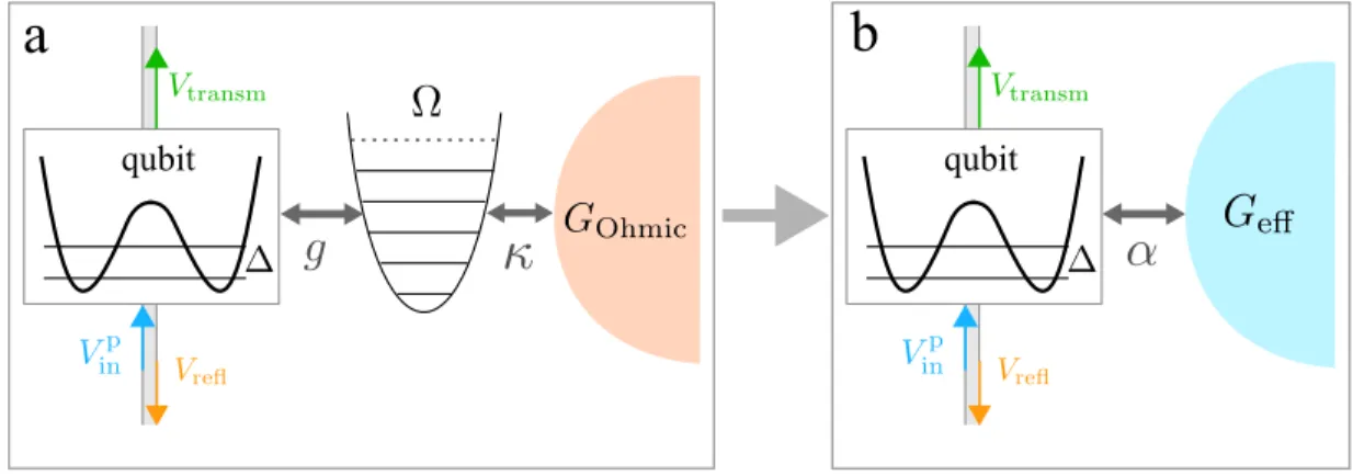
Fig. 1. a - Scheme of the setup analyzed. A flux qubit, probed through a transmission line, is coupled to a resonator, the harmonic oscillator of frequency Ω. The latter is in turn in contact with a Ohmic heat bath. The incoming probe field V

is scattered at the qubit position, resulting in a transmitted and a reflected field. b - Mapping to the spin-boson model. The harmonic bath is described by the structured effective spectral density of Eq. (6), with effective coupling α.

a bosonic heat bath according to the scheme in Fig. 1-a. The qubit is characterized by the frequency scale ∆. The resonator is modeled as a harmonic oscillator of frequency Ω and the frequency g is the qubit-resonator coupling. The resonator is in contact with a dissipative environment modeled as a strictly Ohmic bath with spectral density G

(ω) = κω, where the dimensionless parameter κ quantifies the overall oscillator-bath coupling. The resulting system is described by the dissipative Rabi Hamiltonian, namely by Eq. (1) with H

(t) ≡ H

(t), where

H

(t) = − ~

2 [∆σ

+ ε(t)σ

] + ~ΩB

B + ~gσ

(B

+ B) , (3)

and with ˆ A

= ~ (B

+ B). Here, B

and B are the resonator mode operators and the operators

σ

are the Pauli spin operators in the qubit basis. The qubit parameters, with dimensions of

an angular frequency, are the time-dependent bias ε(t) and the bare qubit frequency splitting at zero bias ∆. In a truncated double-well potential realization of the two-level system, which is proper of flux qubits, ∆ is the tunneling amplitude per unit time of the isolated qubit. The qubit bias ε(t) is (weakly) driven by an incoming probe field through a transmission line which is an independent part of the setup.

Within Van Vleck perturbation theory [37, 38], with g treated as a small parameter with respect to ∆ and Ω, the spectrum of the Rabi Hamiltonian in Eq. (3), can be calculated ana- lytically [39]. In the unbiased case, ε(t) = 0, the eigenfrequencies of the ground state and of the first two excited states read

ω

= − ∆

2 − f (Ω) ω

= Ω

2 − f (Ω) ∓ 1 2

p [∆ − Ω + 2f (Ω)]

+ 4g

,

(4)

with f (Ω) = g

∆

[∆

(∆ + Ω)]

. For Ω = ∆, i.e. at zero detuning, the spectrum presents avoided crossings, see Fig. 2-b below, and the difference ω

− ω

' 2g is the so-called vacuum Rabi splitting, see [40, 41] for experimental observations. Van Vleck perturbation theory can also be used at arbirtary coupling, and thus in the USC regime, also in the presence of a static bias, by treating the qubit energy splitting as a small parameter [42].

The dissipative Rabi Hamiltonian given by Eqs. (1) and (3) can be mapped, see Fig. 1-b, to the Hamiltonian of the SBM [15, 43]

H

(t) = − ~

2 [∆σ

+ ε(t)σ

] − ~ 2 σ

X

k

λ

(a

+ a

) + X

k

~ ω

a

a

, (5) where the qubit is directly coupled to a structured bosonic bath with an effective spectral density function that, in the continuum limit, reads [36, 44, 45]

G

(ω) = 2αωΩ

(Ω

− ω

)

+ (2Γω)

. (6)

This effective spectral density function has an Ohmic behavior ( ∝ ω) at low frequencies, ω/Ω

1, and features a Lorentzian peak centered at the oscillator frequency Ω with semi-width Γ =

πκΩ, with κ the oscillator-bath coupling strength. The effective coupling strength between the

qubit and the structured bath is given by the dimensionless parameter α = 8κg

/Ω

. Note that

for large Ω the Ohmic case with weak coupling is recovered from the spectral density in Eq. (6).

Such mapping can be seen as the inverse application of the reaction coordinate mapping, a technique used to deal with open systems in structured environments [46].

III. THE DRIVEN SPIN-BOSON MODEL WITHIN NIBA

The exact time evolution of the qubit population difference P (t) = h σ

(t) i in the SBM is governed by the generalized master equation (GME) [43]

P ˙ (t) = Z

t0

dt

K

(t, t

) − K

(t, t

)P(t

)

. (7)

The formal exact expression for the kernels can be found within the path integral representa- tion of the qubit reduced density matrix. In the path integral approach, the Feynman-Vernon influence functional [47], which results from tracing out exactly the environmental degrees of freedom, couples the qubit tunneling transitions in a time-nonlocal fashion. The exact kernels of the GME collect all the irreducible sequences of tunneling processes involved in the sum over paths, namely the sequences that cannot be cut into two or more noninteracting parts, the interactions being mediated by the bath correlation function Q(t)

Q(t) = Q

(t) + iQ

(t) = Z

0

dω G(ω) ω

coth

~ ωβ

2

(1 − cos ωt) + i sin ωt

. (8)

This function is related to the bath force operator, or quantum noise, ξ(t) = ˆ

N

X

j=1

c

ˆ

x

(0) cos (ω

t) + p ˆ

(0)

m

ω

sin (ω

t)

(9) which appears in the generalized quantum Langevin equation [48] for a central system coupled to the harmonic environment described in Eq. (1). Here ˆ x

and ˆ p

are position and momentum of the j-th bath oscillator. The bath correlation function Q(t) coincides with the two-time integrated bath force correlation function L(t) = h ξ(t) ˆ ˆ ξ(0) i , i.e., ¨ Q(t) = L(t).

The exact formal expression for the kernels of the GME has no known closed form that can be

used for actual calculations, so that approximation schemes appropriate for the different physical

parameter regimes are introduced. The noninteracting-blip approximation (NIBA) exploits the

fact that the time-nonlocal interactions, the so-called blip-blip interactions mediated by Q(t),

are suppressed at long times and to an extent that increases with the coupling strength to the

heat bath and with the bath temperature. This approximation scheme consists in neglecting these nonlocal interactions and is therefore suited for the strong coupling/high temperature regime. However, at zero bias, ε(t) = 0, an exact cancellation of the blip-blip interactions occurs, so that NIBA yields reasonably accurate results for the population difference also at weak coupling [15, 49].

The time dependent bias ε(t) in the qubit Hamiltonian, see Eq. (3), accounts for an externally applied static flux and the monochromatic, weak probe field. Following [18], we set

ε(t) = ε

+ ε

cos(ω

t) , (10)

with ε

/ω

1. Note that in the actual setup considered in the application of Sec. V, the qubit is not biased, meaning that the applied static flux is tuned so as to have ε

= 0.

In the presence of the time-dipenent bias in Eq. (10), the kernels of the GME (7), within NIBA, read [43]

K

(t, t

) =h

(t − t

) cos

ζ(t, t

) , K

(t, t

) =h

(t − t

) sin

ζ (t, t

) ,

(11)

where the dynamical phase ζ(t, t

) is given by ζ(t, t

) =

Z

t⁰

dt

ε(t

)

=ε

(t − t

) + ε

ω

sin(ω

t) − sin ω

t

,

(12)

and where

h

(t) =∆

e

cos[Q

(t)] , h

(t) =∆

e

sin[Q

(t)] .

(13)

IV. SPECTROSCOPY OF THE QUBIT: RELATING THE MEASURED TRANSMISSION TO THE QUBIT DYNAMICS

As shown in Fig. 1 (see also [18, 50]), a probe voltage field V

(t) = f

ε

cos(ω

t) is scattered

by the qubit placed at the center of the transmission line used to probe the qubit. The constant

f

has dimensions of a flux and the angular frequency ε

is the (small) amplitude of the probe.

The scattering of the incoming probe field V

yields a transmitted and a reflected field, denoted by V

(t) and V

(t), respectively, see Fig. 1. The flux difference across the qubit is δΦ(t) = Φ(0

, t) − Φ(0

, t), with the flux given by Φ(0

, t) = R

−∞

dt

V (0

, t

). Here 0

refers to the positions immediately before and after the position of the qubit in the transmission line.

Following [51], we have for the voltage V (0

, t) and current I (0

, t) immediately before the qubit position the following equations

V (0

, t) = V

(t) + V

(t) , (14) I (0

, t) = 1

Z

V

(t) − V

(t)

, (15)

where Z is the characteristic impedance of the transmission line. Similarly, immediately after the qubit position

V (0

, t) = V

(t) , (16)

I(0

, t) = 1

Z V

(t) . (17)

Using the conservation of the current, I(0

, t) = I(0

, t), and the relation V (0

, t) − V (0

, t) = δΦ(t), we obtain ˙

V

(t) = V

(t) − δΦ(t) ˙

2 . (18)

The connection between the measured transmission, defined as the ratio

T (ω

) = V

(ω

)/V

(ω

) , (19) and the spin-boson dynamics is completed by identifying the flux difference across the qubit with the population difference of the localized eigenstates of the flux operator ˆ Φ = f σ

, namely by setting δΦ(t) ≡ f h σ

(t) i , with f a proportionality constant with dimension of a flux.

Since we want to connect the asymptotic, time-periodic dynamics induced by the probe field – and rendered by the GME (7) – to the measured transmission, we start by considering the asymptotic population difference P

(t) = lim

P (t). Due to its periodicity, with period 2π/ω

, we can express it as a Fourier series whose time derivative reads

P ˙

(t) = X

m

imω

p

e

, (20)

where

p

= ω

2π

Z

−π/ωp

dt P

(t)e

. (21) In the asymptotic limit we set δΦ(t) ≡ f P

(t). Then, the transmission at the probe frequency ω

(m = 1 in Eq. (20)) obtained by plugging Eq. (18) into Eq. (19), is given by

T (ω

) = f

ε

/2 − if ω

p

/2 f

ε

/2

=1 − i N ω

p

/ε

,

(22)

where N = f /f

. The parameter N can be estimated in experiments and will be set to an arbitrary value in the application of Sec. V.

Due to the effect of the monochromatic probe, the asymptotic population P

(t) is periodic with the period of the probe. Moreover, since the probe is weak (ε

/ω

1), we can confine ourselves to the linear response regime, which amounts to neglecting terms of order higher than the first in the ratio ε

/ω

in the series for P

(t). Denoting with

the first order, we obtain [43, 52]

P

(t) ' p

+ p

e

+ p

e

≡ P

+ ~ε

[χ(ω

)e

+ χ( − ω

)e

] , (23) where we have introduced the linear susceptibility

χ(ω) = p

/ ~ ε

(24)

and where P

is the equilibrium value of P(t) in the static system. We can then relate the transmission at the probe frequency in linear response to the linear susceptibility via the relation T (ω

) = 1 − i N ~ ω

χ(ω

) . (25) A this point we use the GME (7) to find the explicit expression for p

in terms of the NIBA kernels. By substituting Eq. (23) and its time derivative in the limit t → ∞ of the GME (7), we arrive at the closed expression for p

[43, 52]

p

(ω

) = 1 iω

+ v

(ω

)

"

k

(ω

) − k

(ω

) k

k

#

, (26)

where the superscripts 0 and 1 denote zeroth and first order in ε

/ω

, respectively. Note that this expression for p

does not descend from a Markovian limit of the GME, which would yield v

(0) instead of v

(ω

) at the denominator in the prefactor. The kernels k

and v

in Eq. (26) read

k

(ω

) = ω

2π Z

−π/ωp

dt e

Z

0

dτ K

(t, t − τ ) , v

(ω

) = ω

2π Z

−π/ωp

dt Z

0

dτ e

K

(t, t − τ ) ,

(27)

where K

(t, t

) are defined in Eq. (11). Due to the integrations over the probe period 2π/ω

, the dynamical phase ζ(t, t

) in K

(see Eq. (12)) yields the Bessel functions J

[(2ε

/ω

) sin(ω

t/2)]

in the coefficients of k

and v

. The small amplitude of the probe field allows for expanding to lowest order in ε

/ω

the Bessel function by means of J

(x) ∼ (x/2)

, obtaining the following explicit expressions

k

= Z

0

dt h

(t) cos(ε

t) , k

=

Z

0

dt h

(t) sin(ε

t) , k

(ω

) = − ε

ω

Z

0

dt e

h

(t) sin(ε

t) sin(ω

t/2) , k

(ω

) = ε

ω

Z

0

dt e

h

(t) cos(ε

t) sin(ω

t/2) , and v

(ω

) =

Z

0

dt e

h

(t) cos(ε

t) .

(28)

Within the present linear response treatment, the transmission is independent of the probe

amplitude ε

, see Eq. (25). Note that, while the theory presented here assumes a small probe

amplitude, it allows to describe the situation in which the qubit is strongly coupled to its

environment. Moreover, the transmission spectrum of the qubit can be calculated also in the

presence of a pump drive, as in [18], at least in the regime where the drive frequency is much

larger than the renormalized value ∆

of the qubit parameter ∆. This condition is not restrictive

in the strong coupling regime to Ohmic or sub-Ohmic baths (G(ω) ∝ ω

, with s ≤ 1), which

yields a strong renormalization and thus a small ∆

[15]. At finite temperatures, the strong

coupling regime makes the NIBA perform satisfactorily also in the presence of a static bias.

V. RESULTS

In this section we apply the formalism reviewed above to the setup shown in Fig. 1-a, where the static bias is zero, ε

= 0. This entails that k

= k

= 0 in Eq. (28). The resulting expression for the susceptibility simplifies to

χ(ω

) = 1

~ε

k

(ω

)

iω

+ v

(ω

) . (29)

The effective spectral density in Eq. (6), yields for the real and imaginary parts Q

(t) and Q

(t) of the bath correlation function in Eq. (8) the exlpicit expressions [49]

Q

(t) = Xτ − L e

cos ¯ Ωτ − 1

− Ze

sin ¯ Ωt + Q

(t) , (30) Q

(t) = πα − e

πα cos ¯ Ωt − N sin ¯ Ωt

, (31)

with X = 2παk

T / ~ and ¯ Ω = √

Ω

− Γ

and where N = Ω

− 2Γ

2Γ ¯ Ω ,

L = πα N sinh (β ~ Ω) ¯ − sin (β ~ Γ) cosh (β ~ Ω) ¯ − cos (β ~ Γ) , Z = πα sinh (β ~ Ω) + ¯ N sin (β ~ Γ)

cosh (β ~ Ω) ¯ − cos (β ~ Γ) .

(32)

The term Q

(t) is the following series over the Matsubara frequencies ν

:= n 2πk

T / ~ Q

(t) = 4πα Ω

~β

+∞

X

n=1

1

(Ω

+ ν

)

− 4Γ

ν

1 − e

ν

. (33)

In what follows, we set the parameter that relates, according to Eq. (25), the calculated suscep- tibility to the measured transmission T at the probe frequency to the value N = 0.1. Moreover, while varying the resonator frequency Ω and qubit-resonator coupling g, we fix the resonator- bath coupling to κ = 0.05. Finally, the temperature of the bath is chosen to be T = ~∆/k

.

In Fig. 2, we show the full qubit transmission spectrum with the qubit-resonator coupling set

to g = 0.2 ∆, namely in the USC regime. Specifically, the transmission |T |

is calculated as a

function of the oscillator frequency Ω and of the probe frequency ω

. The transition frequencies

ω

= ω

− ω

and ω

= ω

− ω

of the non-dissipative model, from Eq. (4), are also shown along

with the corresponding quantities for the uncoupled system, g = 0, to highlight the presence of

0 0.5 1 1.5 2

0.5 1 1.5

ω

/ ∆

Ω/∆

0.7 0.8 0.9 1

|T |

a)

0 0.5 1

0.5 1 1.5

ω

(Ω) ω

(Ω) ω

(Ω

) ω

(Ω) b)

Ω/∆

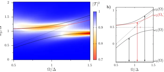
Fig. 2. a - Transmission |T |

as a function of the resonator frequency Ω and probe frequency ω

. Parameters are g = 0.2 ∆, κ = 0.05, T = ~∆/k

, and N = 0.1. Black solid lines - Transition frequencies ω

(Ω) and ω

(Ω), from the spectrum of the non-dissipative Rabi model, see Eq. (4). Red solid line - Transition frequency ω

(Ω

), where we assumed Ω

= 0.87 Ω, which yields the resonance condition at Ω ' 1.15 ∆. Dashed lines - transition frequencies for the decoupled qubit-resonator system, g = 0. b - Eigenfrequencies of the coupled and uncoupled system and transition frequencies (arrows). The black and red tics on the horizontal dashed line indicate the resonance conditions Ω = ∆ and Ω

= ∆, respectively.

Note that Eq. (4) is a perturbative result valid for g ∆, Ω.

the avoided crossing at the resonance condition Ω = ∆. In the regions where the transmission is not complete, |T |

< 1, the qubit response to the probe is different from zero, meaning that the qubit dynamics has a component at the probe frequency.

To appreciate the features of the transmission plotted in Fig. 2, we first describe the fea- tures of the qubit dynamics given by the population difference in Fourier space, F (ω) = 2 R

0

dt cos(ωt)P (t), as analyzed in [39] for the non-dissipative and the weakly dissipative cases

in the absence of a probe field. In the non-dissipative case, F (ω) is characterized by a sequence

of peaks with two dominating contributions at ω

and ω

, the two frequencies being sepa-

rated, at resonance, by the vacuum Rabi splitting 2g. In the presence of a weak dissipation,

κ = 0.015 and T = 0.1 ~ ∆/k

, the secondary peaks are washed out and the two main peaks are broadened. Moreover, the relative magnitude of the peaks depends on the detuning ∆ − Ω.

This can be accounted for within a Bloch-Redfield master equation approach: One finds that the contribution to F (ω) at frequency ω

, with n = 1, 2, is weighted by the factor Γ

, where Γ

are the dephasing rates in the full secular approximation. Evaluation of the dephasing rates shows that negative detuning yields Γ

> Γ

and thus a larger contribution of the peak at the higher frequency, whereas positive detuning yields a dominating peak at the lower frequency.

These features are qualitatively present in the corresponding behavior of the transmission

shown in Fig. 2 for the stronger dissipation/higher temperature regime considered here. There

are however interesting peculiarities that arise from the interplay between the detuning and

dissipation. Indeed, due to the coupling to the heat bath, the resonator frequency is renor-

malized to Ω

< Ω. As a result, the resonance condition Ω

= ∆ occurs at some value of Ω

larger than ∆. This is reflected by the fact that the simultaneous presence of two dips in the

transmission, expected at Ω ' ∆ for weak dissipation, here occurs around the value 1.15 ∆. The

renormalization of the oscillator frequency also accounts for the fact that, for Ω & ∆, the trace

of the dip at the lower frequency is well reproduced by the curve ω

(Ω) while the one at the

higher frequency is reproduced by ω

(Ω

), where we assume the simple relation Ω

= 0.87 Ω

in order to have the resonant condition at Ω ' 1.15 ∆, see the red solid line in Fig. 2. The

shift of the dip positions is non-symmetric because the transition frequency ω

is more affected

by the renormalization of the oscillator frequency than ω

. The reason is that the dominant

contributions to the eigenfrequencies in Eq. (4) come from the uncoupled case, g = 0, which

gives ω

= Ω and ω

= ∆ at positive detuning (Ω > ∆). As a result of this non-symmetric

shift, around the resonance the distance between the dips is less than the vacuum Rabi splitting

2g. The renormalization towards lower values of the oscillator frequency also enhances the loss

of accuracy at low Ω of the perturbative calculation (g ∆, Ω) yielding the eigenfrequencies

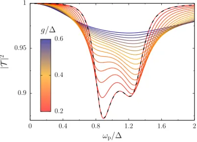
in Eq. (4). At the extrema of the Ω-range we notice that just one of the two dips in the trans-

mission survives. At small resonator frequencies, Ω ' 0.5 ∆, the transmission displays a single,

broad dip centered at ω

' 1.2 ∆. The large broadening is consistent with the fact that, by

decreasing Ω, the effective coupling α between the qubit and the structured spectral density in

0.7 0.8 0.9 1

0 0.4 0.8 1.2 1.6 2

Ω/∆

a)

|T|2

ωp/∆

0.5 1 1.5

0.8 0.9 1

0 0.5 1 1.5 2

α

b)

0.8 0.9 1

1

|T|2

ωp/∆

0.03 0.12 0.21

ωp/∆T

Fig. 3. Transmission |T |

as a function of the probe frequency ω

. a - Qubit-dissipative resonator system for different values of the resonator frequency Ω. Parameters are the same as in Fig. 2. The relative weight of the dips is dictated by the detuning with respect to the renormalized resonator frequency Ω

. The dip at high (low) frequency dominates for Ω

< ∆ ( Ω

> ∆). The dashed line is at Ω = 1.2 ∆. b - Qubit directly coupled to an Ohmic bath for different values of the coupling strength α. Bath temperature and cutoff frequency are T = ~∆/k

and ω

= 10 ∆, respectively, and N = 0.1. Inset - Transmission vs.

the probe frequency scaled with the temperature-dependent renormalized qubit splitting ∆

of Eq. (34):

The dips in the transmission are centered at ω

= ∆

.

Eq. (6) increases. In the opposite limit, around Ω = 1.5 ∆, there is a single, narrow dip centered towards Ω = ∆, consistently with the fact that at large Ω the effective spectral density of Eq. (6) reproduce a weakly coupled Ohmic bath.

These features are best seen in Fig. 3-a, where the transmission is shown as a function of

the probe frequency for different values of the resonator frequency Ω, from negative to positive

detuning Ω

− ∆, with the same parameters as in the colormap of Fig. 2. The curves show,

around the resonance condition Ω

' ∆, the (broadened) two-dip pattern characteristic of the

qubit-oscillator system. At large values of Ω the spectra present a single narrow dip at a fre-

quency which tends to the position ω

= ∆, as the effective coupling α decreases by increasing

Ω. In the opposite regime of small Ω, the effective coupling α tends to be large and the doubly

peaked structure is smoothed out to leave a single broad dip centered at ω

' 1.2 ∆. This

upwards renormalization of the qubit splitting due to the structured environment beyond weak

dissipation has been already observed in [53] using the flow-equation renormalization group ap- proach. It is in striking contrast with the downwards renormalization of ∆ occurring in the Ohmic case, whereby upon increasing the coupling to the heat bath, the dip in the transmission also broadens but tends to lower frequencies. This point is exemplified by Fig. 3-b where, for comparison, the transmission is shown for the qubit directly coupled to a Ohmic bath with spectral density function G

= 2αω exp( − ω/ω

), for different values of the qubit-bath cou- pling α. In the temperature/coupling regime considered in Fig. 3-b, the temperature-dependent

0.9 0.95 1

0 0.4 0.8 1.2 1.6 2

g/∆

|T |

ω

/∆

0.2 0.4 0.6

Fig. 4. Transmission |T |

as a function of the probe frequency ω

for different values of the qubit- resonator coupling g. The resonators frequency is Ω = 1.2 ∆ and the remaining parameters are as in Fig. 2. The separation between the peaks increases as g is increased. The dashed curves here and in Fig. 3-a are obtained with the same set of parameters and thus coincide. Increasing g, the separation between the dips increases and the dip at high frequency becomes the dominant.

renormalization of the qubit frequency splitting for the Ohmic bath is given by [15]

∆

= ∆

(ν

/∆

)

, (34)

with ∆

= ∆(∆/ω

)

the renormalized splitting at T = 0 and ν

= 2πk

T / ~ the first

Matsubara frequency. As shown in the inset of Fig. 3-b, by scaling the probe frequency with

this renormalized splitting, the positions of the dips at different α collapse to the value 1.

We complement the information provided in Figs. 2 and 3 with the curves of Fig. 4, where the qubit-resonator coupling g is increased from 0.2 to 0.6, in units of ∆, with Ω fixed to the value 1.2 ∆. While for the lower values of coupling the dip the low-frequency dip is dominant, by increasing g, the dip at the higher frequency dominates. At large qubit-resonator coupling, the two-dip structure is smoothed out resulting in a single, broad dip centered at ω

> ∆, similarly to what happens by decreasing Ω at fixed g.

The present analysis can be pushed towards lower coupling strengths and temperatures, where the NIBA is still reliable for the unbiased system, see for example the analytical weak damping approximation, derived within NIBA in [49]. Moreover, at low temperatures and weak qubit- oscillator coupling, an analytical treatment beyond the rotating-wave approximation, which accounts also for a static bias, ε

6 = 0, is provided in [39].

As a final remark, we note that, in the present linear response regime to the probe field, the weak time-dependent bias does not spoil the NIBA results. This is because linear response theory reproduces the dissipative dynamics of the static system which is in turn well-described within the NIBA. In [44], the performance of the NIBA with an effective spectral density of the same type as Eq. (6) has been compared with the numerically exact results of QUAPI.

VI. CONCLUSIONS

In recent years, superconducting quantum circuits assumed the role of leading platforms for quantum computing and simulations. In the latter context, a qubit coupled to a super- conducting resonator forms the basic setup for quantum optics experiments in the ultrastrong coupling regime of light and matter. To account for the presence of dissipation, brought in by the coupling of the resonator to a reservoir of bosonic modes, the system can be mapped to a spin-boson system with the distribution of environmental couplings displaying a peak at the oscillator frequency, rendering a so-called structured bath. The noninteracting-blip approxima- tion represents a valuable tool for investigating the qubit reduced dynamics in the presence of dissipation and in the nonperturbative regime of qubit-resonator coupling.

In our work, we employed the tools developed within this approximation scheme to spectro-

scopically analyze the setup of a flux qubit ultrastrongly coupled to a dissipative resonator. The

transmission of a weak probe field, which is measured in actual experiments, is connected to the qubit dynamics under the influence of the resonator-bath system, via a linear response treat- ment. We investigated how dissipation in the resonator affects the qubit transmission spectra by varying the qubit-resonator detuning and its coupling to the qubit. The interaction between the resonator and a heat bath beyond the weak coupling limit introduces a renormalization of the resonator frequency which, in turn, modifies the qubit response. We find a bath-induced shift of the resonance condition and a decreased vacuum Rabi splitting, due to the fact that the renormalization of the oscillator frequency affects the relevant transitions in a non-symmetric way. Moreover, the broadening of the dips in the transmission, which is due to dissipation, depends on the qubit-resonator detuning. Finally, an upwards renormalization effect of the qubit splitting is found at small resonator frequencies, witnessing the structured nature of the effective environment of the qubit.

The study performed here can be extended to multiple baths and different coupling setups and the formalism can account for the presence of driving in the qubit parameters. In recent years, a two-bath version of the spin-boson model has been explored in the context of heat transfer between heat baths [54–62]. The formalism used here is suitable for describing a setup for heat transport in the quantum regime of the same kind of the one realized in [32], where a qubit is connected to two heat baths at different temperatures via waveguide resonators.

ACKNOWLEDGMENTS

The authors acknowledge financial support by the Deutsche Forschungsgemeinschaft via SFB 1277 B02.

References

[1] J. Q. You and F. Nori, “Atomic physics and quantum optics using superconducting circuits,” Nature

474, 589–597 (2011).

[2] A. A. Houck, H. E. T¨ ureci, and J. Koch, “On-chip quantum simulation with superconducting circuits,” Nat. Phys. 8, 292 (2012).

[3] J. P. Pekola, “Towards quantum thermodynamics in electronic circuits,” Nat. Phys. 11, 118 (2015).

[4] G. Wendin, “Quantum information processing with superconducting circuits: a review,” Rep. Prog.

Phys. 80 , 106001 (2017).

[5] X. Gu, A. F. Kockum, A. Miranowicz, Y.-X. Liu, and F. Nori, “Microwave photonics with super- conducting quantum circuits,” Phys. Rep. 718-719, 1–102 (2017).

[6] T. Niemczyk, F. Deppe, H. Huebl, P. E. Menzel, F. Hocke, J. M. Schwarz, J. J. Garc´ıa-Ripoll, D. Zueco, T. H¨ ummer, E. Solano, A. Marx, and R. Gross, “Circuit quantum electrodynamics in the ultrastrong-coupling regime,” Nat. Phys. 6, 772 (2010).

[7] S. Ashhab and F. Nori, “Qubit-oscillator systems in the ultrastrong-coupling regime and their po- tential for preparing nonclassical states,” Phys. Rev. A 81, 042311 (2010).

[8] P. Forn-D´ıaz, J. Lisenfeld, D. Marcos, J. J. Garc´ıa-Ripoll, E. Solano, C. J. P. M. Harmans, and J. E. Mooij, “Observation of the Bloch-Siegert Shift in a Qubit-Oscillator System in the Ultrastrong Coupling Regime,” Phys. Rev. Lett. 105 , 237001 (2010).

[9] F. Yoshihara, T. Fuse, S. Ashhab, K. Kakuyanagi, S. Saito, and K. Semba, “Superconducting qubit-oscillator circuit beyond the ultrastrong-coupling regime,” Nat. Phys. 13, 44 (2016).

[10] F. Yoshihara, T. Fuse, S. Ashhab, K. Kakuyanagi, S. Saito, and K. Semba, “Characteristic spectra of circuit quantum electrodynamics systems from the ultrastrong- to the deep-strong-coupling regime,”

Phys. Rev. A 95, 053824 (2017).

[11] P. Forn-D´ıaz, L. Lamata, E. Rico, J. Kono, and E. Solano, “Ultrastrong coupling regimes of light- matter interaction,” Rev. Mod. Phys. 91, 025005 (2019).

[12] F. A. Kockum, A. Miranowicz, S. De Liberato, S. Savasta, and F. Nori, “Ultrastrong coupling between light and matter,” Nat. Rev. Phys. 1, 19–40 (2019).

[13] M. H. Devoret and J. M. Martinis, “Implementing Qubits with Superconducting Integrated Circuits,”

Quant. Inf. Proc. 3 , 163–203 (2004).

[14] A. J. Leggett, S. Chakravarty, A. T. Dorsey, M. P. A. Fisher, A. Garg, and W. Zwerger, “Dynamics of the dissipative two-state system,” Rev. Mod. Phys. 59, 1–85 (1987).

[15] U. Weiss, Quantum Dissipative Systems (World Scientific, Singapore, 2012, 4th ed.).

[16] H. P. Breuer and F. Petruccione, The theory of open quantum systems (Oxford University Press, Oxford, 2002).

[17] P. Forn-D´ıaz, J. J. Garc´ıa-Ripoll, B. Peropadre, J. L. Orgiazzi, M. A. Yurtalan, R. Belyansky, C. M.

Wilson, and A. Lupascu, “Ultrastrong coupling of a single artificial atom to an electromagnetic

continuum in the nonperturbative regime,” Nat. Phys. 13, 39–43 (2017).

[18] L. Magazz` u, P. Forn-D´ıaz, R. Belyansky, J.-L. Orgiazzi, M. A. Yurtalan, M. R. Otto, A. Lupascu, C. M. Wilson, and M. Grifoni, “Probing the strongly driven spin-boson model in a superconducting quantum circuit,” Nat. Commun. 9, 1403 (2018).

[19] J. Lepp¨ akangas, J. Braum¨ uller, M. Hauck, J.-M. Reiner, I. Schwenk, S. Zanker, L. Fritz, A. V.

Ustinov, M. Weides, and M. Marthaler, “Quantum simulation of the spin-boson model with a microwave circuit,” Phys. Rev. A 97, 052321 (2018).

[20] P. M. Javier, L. S´ebastien, N. Gheeraert, R. Dassonneville, L. Planat, F. Foroughi, Y. Krupko, O. Buisson, C. Naud, W. Hasch-Guichard, S. Florens, I. Snyman, and N. Roch, “A tunable Joseph- son platform to explore many-body quantum optics in circuit-QED,” npj Quantum Inf. 5, 19 (2019).

[21] R. Kuzmin, N Mehta, N. Grabon, R. Mencia, and V. E. Manucharyan, “Superstrong coupling in circuit quantum electrodynamics,” npj Quantum Inf. 5, 20 (2019).

[22] D. Z. Rossatto, C. J. Villas-Bˆ oas, M. Sanz, and E. Solano, “Spectral classification of coupling regimes in the quantum Rabi model,” Phys. Rev. A 96, 013849 (2017).

[23] L. Garziano, R. Stassi, V. Macr`ı, A. F. Kockum, S. Savasta, and F. Nori, “Multiphoton quantum Rabi oscillations in ultrastrong cavity QED,” Phys. Rev. A 92 , 063830 (2015).

[24] G. D´ıaz-Camacho, A. Bermudez, and J. J. Garc´ıa-Ripoll, “Dynamical polaron ansatz: A theoretical tool for the ultrastrong-coupling regime of circuit QED,” Phys. Rev. Lett. 93, 043843 (2016).

[25] F. Armata, G. Calajo, T. Jaako, M. S. Kim, and P. Rabl, “Harvesting multiqubit entanglement from ultrastrong interactions in circuit quantum electrodynamics,” Phys. Rev. Lett. 119, 183602 (2017).

[26] D. De Bernardis, P. Pilar, T. Jaako, S. De Liberato, and P. Rabl, “Breakdown of gauge invariance in ultrastrong-coupling cavity QED,” Phys. Rev. A 98, 053819 (2018).

[27] O. Di Stefano, A. Settineri, V. Macr`ı, L. Garziano, R. Stassi, S. Savasta, and F. Nori, “Resolution of gauge ambiguities in ultrastrong-coupling cavity quantum electrodynamics,” Nat. Phys. 15 , 803–808 (2019).

[28] F. Beaudoin, J. M. Gambetta, and A. Blais, “Dissipation and ultrastrong coupling in circuit QED,”

Phys. Rev. A 84, 043832 (2011).

[29] I. Chiorescu, P. Bertet, K. Semba, Y. Nakamura, C. J. P. M. Harmans, and J. E. Mooij, “Coherent dynamics of a flux qubit coupled to a harmonic oscillator,” Nature 431, 159–162 (2004).

[30] M. Thorwart, E. Paladino, and M. Grifoni, “Dynamics of the spin-boson model with a structured

environment,” Chem. Phys 296, 333–344 (2004).

[31] J. Johansson, S. Saito, T. Meno, H. Nakano, M. Ueda, K. Semba, and H. Takayanagi, “Vacuum Rabi Oscillations in a Macroscopic Superconducting Qubit LC Oscillator System,” Phys. Rev. Lett.

96, 127006 (2006).

[32] A. Ronzani, B. Karimi, J. Senior, Y.-C. Chang, J. T. Peltonen, C.D. Chen, and J. P. Pekola,

“Tunable photonic heat transport in a quantum heat valve,” Nat. Phys. 14 , 991–995 (2018).

[33] J. Lolli, A. Baksic, D. Nagy, V. E. Manucharyan, and C. Ciuti, “Ancillary qubit spectroscopy of vacua in cavity and circuit quantum electrodynamics,” Phys. Rev. Lett. 114, 183601 (2015).

[34] G. Falci, A. Ridolfo, P. G. Di Stefano, and E. Paladino, “Ultrastrong coupling probed by coherent population transfer,” Sci. Rep. 9, 9249 (2019).

[35] A. Ridolfo, G. Falci, F. M. D. Pellegrino, G. D. Maccarrone, and E. Paladino, “Photon pair pro- duction by STIRAP in ultrastrongly coupled matter-radiation systems,” Eur. Phys. J. Spec. Top.

227, 2183 (2019).

[36] A. Garg, J. N. Onuchic, and V. Ambegaokar, “Effect of friction on electron transfer in biomolecules,”

J. Chem. Phys. 83, 4491–4503 (1985).

[37] J. H. Van Vleck, “On σ-Type Doubling and Electron Spin in the Spectra of Diatomic Molecules,”

Phys. Rev. 33 , 467–506 (1929).

[38] C. Cohen-Tannoudji, J. Dupont-Roc, and G. Grynberg, Atom-Photon Interactions: Basic Processes and Applications (Wiley-VCH, New York, 1998).

[39] J. Hausinger and M. Grifoni, “Dissipative dynamics of a biased qubit coupled to a harmonic oscilla- tor: analytical results beyond the rotating wave approximation,” New J. Phys. 10, 115015 (2008).

[40] A. Wallraff, D. I. Schuster, A. Blais, L. Frunzio, R.-S. Huang, J. Majer, S. Kumar, S. M. Girvin, and R. J. Schoelkopf, “Strong coupling of a single photon to a superconducting qubit using circuit quantum electrodynamics,” Nature 431, 162–167 (2004).

[41] A. Fragner, M. G¨oppl, J. M. Fink, M. Baur, R. Bianchetti, P. J. Leek, A. Blais, and A. Wallraff,

“Resolving Vacuum Fluctuations in an Electrical Circuit by Measuring the Lamb Shift,” Science 322 , 1357 (2008).

[42] J. Hausinger and M. Grifoni, “Qubit-oscillator system: An analytical treatment of the ultrastrong coupling regime,” Phys. Rev. A 82, 062320 (2010).

[43] M. Grifoni and P. H¨anggi, “Driven quantum tunneling,” Phys. Rep. 304, 229–354 (1998).

[44] M. C. Goorden, M. Thorwart, and M. Grifoni, “Entanglement Spectroscopy of a Driven Solid-State Qubit and Its Detector,” Phys. Rev. Lett. 93, 267005 (2004).

[45] D. Zueco and J. J. Garc´ıa-Ripoll, “Ultrastrongly dissipative quantum Rabi model,” Phys. Rev. A

99, 013807 (2019).

[46] R. Martinazzo, B. Vacchini, B., K. H. Hughes, and I. Burghardt, “Communication: Universal Markovian reduction of Brownian particle dynamics,” J. Chem. Phys. 134, 011101 (2011).

[47] R. P Feynman and F. L. Vernon Jr., “The theory of a general quantum system interacting with a linear dissipative system,” Ann. Phys. (N.Y.) 24, 118–173 (1963).

[48] P. H¨ anggi and G.-L. Ingold, “Fundamental aspects of quantum Brownian motion,” Chaos 15 , 26105 (2005).

[49] F. Nesi, M. Grifoni, and E. Paladino, “Dynamics of a qubit coupled to a broadened harmonic mode at finite detuning,” New J. Phys. 9, 316–316 (2007).

[50] B. Peropadre, J. Lindkvist, I.-C. Hoi, C. M. Wilson, J. J. Garc´ıa-Ripoll, P. Delsing, and G. Johans- son, “Scattering of coherent states on a single artificial atom,” New J. Phys. 15, 035009 (2013).

[51] U. Vool and M. Devoret, “Introduction to quantum electromagnetic circuits,” Int. J. Circ. Theor.

Appl. 45, 897–934 (2017).

[52] M. Grifoni, M. Sassetti, P. H¨ anggi, and U. Weiss, “Cooperative effects in the nonlinearly driven spin-boson system,” Phys. Rev. E 52, 3596–3607 (1995).

[53] S. Kleff, S. Kehrein, and J. von Delft, “Exploiting environmental resonances to enhance qubit quality factors,” Phys. Rev. B 70 , 014516 (2004).

[54] L. Nicolin and D. Segal, “Non-equilibrium spin-boson model: Counting statistics and the heat exchange fluctuation theorem,” J. Chem. Phys. 135, 164106 (2011).

[55] N. Boudjada and D. Segal, “From Dissipative Dynamics to Studies of Heat Transfer at the Nanoscale:

Analysis of the Spin-Boson Model,” J. Phys. Chem. A 118, 11323–11336 (2014).

[56] D. Segal, “Heat transfer in the spin-boson model: A comparative study in the incoherent tunneling regime,” Phys. Rev. E 90, 012148 (2014).

[57] R. Schmidt, M. F. Carusela, J. P. Pekola, S. Suomela, and J. Ankerhold, “Work and heat for two-level systems in dissipative environments: Strong driving and non-Markovian dynamics,” Phys.

Rev. B 91 , 224303 (2015).

[58] M. Carrega, P. Solinas, A. Braggio, M. Sassetti, and U. Weiss, “Functional integral approach to time-dependent heat exchange in open quantum systems: general method and applications,” New J. Phys. 17, 045030 (2015).

[59] M. Carrega, P. Solinas, M. Sassetti, and U. Weiss, “Energy Exchange in Driven Open Quantum Systems at Strong Coupling,” Phys. Rev. Lett. 116, 240403 (2016).

[60] C. Wang, J. Ren, and J. Cao, “Unifying quantum heat transfer in a nonequilibrium spin-boson

model with full counting statistics,” Phys. Rev. A 95, 023610 (2017).

[61] B. K. Agarwalla and D. Segal, “Energy current and its statistics in the nonequilibrium spin-boson model: Majorana fermion representation,” New J. Phys. 19, 043030 (2017).

[62] D. Newman, F. Mintert, and A. Nazir, “Performance of a quantum heat engine at strong reservoir

coupling,” Phys. Rev. E 95, 032139 (2017).