Extending Freeze-LTL on Multi-Attributed Data Words with Quantifiers Erweiterung von Freeze-LTL auf mehrfach attributierten Datenwörtern um Quantoren

Extending Freeze-LTL on Multi-Attributed Data Words with Quantifiers

Erweiterung von Freeze-LTL auf mehrfach attributierten Datenwörtern um Quantoren

Bachelorarbeit

im Rahmen des Studiengangs Informatik

der Universität zu Lübeck

vorgelegt von Anton Pirogov

ausgegeben und betreut von Prof. Dr. Martin Leucker mit Unterstützung von Normann Decker

Lübeck, den 15. Juli 2015

Erklärung

Hiermit erkläre ich an Eides statt, dass ich die vorliegende Arbeit ohne unzulässige Hilfe Dritter und ohne die Benutzung anderer als der angegebenen Hilfsmittel selbständig verfasst habe; die aus anderen Quellen direkt oder indirekt übernommenen Daten und Konzepte sind unter Angabe des Literaturzitats gekennzeichnet.

(Anton Pirogov)

Lübeck, den 15. Juli 2015

Abstract The family of temporal logics is useful to precisely specify the behaviour of systems with relation to time. For example, that some events have to follow each other, always or never happen, etc. They are often used in the context of software verification to test programs for correct behaviour, because not all errors can be caught at compile time or by unit tests. From corresponding logical formulae one can for example construct efficient monitors that evaluate the execution of programs and can detect whether there are deviations from the specification.

These logics differ in expressivity, depending on the allowed operators and quantifiers. So the ambition is to construct logics that allow for expression of interesting properties while keeping the verification or at least decidability feasible. The logic Freeze-LTL extends LTL and allows for storing a value in a register and checking for equality at some later point in time. The main contribution of this thesis is the definition of a new logic and the proof that decidability is preserved. This logic combines two different extensions of Freeze-LTL from the literature – on the one hand, the possibility to work with multiple ordered attributes, if they exhibit a kind of hierarchial structure, on the other hand, the possibility to quantify over previous values or guess some future value for which some property must hold.

Kurzfassung Die Familie der linearen Temporallogiken eignet sich hervorragend dazu, das Verhalten von Systemen in Abhängigkeit von Zeit präzise zu beschreiben bzw. spez- ifizieren. Zum Beispiel, dass bestimmte Ereignisse aufeinander folgen müssen, immer oder nie eintreten, etc. Sie werden oft im Kontext der Softwareverifikation verwendet, um Programme auf korrektes Verhalten zu prüfen, da sich nicht alle Fehler bereits zur Kompilierzeit oder durch statische Unit-Tests erkennen lassen. Aus entsprechenden lo- gischen Formeln können dann zum Beispiel effiziente Monitore generiert werden, welche die beschriebenen Programme zur Laufzeit überwachen und feststellen können, ob es Abweichungen von der Spezifikation gibt.

Diese Logiken können je nach erlaubten Operatoren und Quantoren unterschiedlich aus- drucksstark sein. Es gilt also, möglichst Logiken zu konstruieren, welche einem erlauben, interessante Eigenschaften auszudrücken und dabei möglichst einfach überprüfbar oder überhaupt entscheidbar bleiben. Die auf LTL basierende Logik Freeze-LTL erlaubt das Speichern eines Wertes in einem Register und eine spätere Prüfung auf Gleichheit. In dieser Arbeit wird eine neue Logik definiert und es wird gezeigt, dass Entscheidbarkeit in der resultierenden Logik gewahrt bleibt. Diese Logik kombiniert zwei unterschiedliche Erweiterungen von Freeze-LTL – einerseits die Möglichkeit, mit mehreren geordneten Attributen zu arbeiten, solange diese eine gewisse hierarchische Struktur aufweisen, andererseits die Möglichkeit, über vergangene Werte zu quantifizieren oder einen zukün- ftigen Wert zu raten, für den oder die dann etwas gelten soll.

Contents

1 Introduction 1

1.1 Background and related work . . . 1

1.2 Contribution of this thesis . . . 4

2 Definition of the logic 5 2.1 Preliminaries . . . 5

2.2 Syntax and semantics . . . 11

3 Nested Register Automata 15 3.1 Definition of NRA . . . 15

3.2 Emptiness of NRA . . . 19

3.2.1 Preliminaries . . . 19

3.2.2 Proof of decidability . . . 24

4 Decidability of the logic 31 4.1 Linearisation fromLTL^↓_AtoLTL^↓_[k] . . . 31

4.2 Translation of formulae to NRA . . . 39

5 Summary and Open Questions 45

1 Introduction

1.1 Background and related work

Our modern world is increasingly dependent on the correct functioning of different technical systems – from electronic household devices to factories producing goods and space stations floting in orbit. As these systems are becoming more and more complex, there is a need for tools that allow to express how we expect these systems to behave and also supervise and evaluate their work. The field of formal verification is researching and providing the world with exactly such tools, enabling us to model different systems, specify the expected behaviour and verify that the actual behaviour does indeed correspond to our model.

As such systems are mostly implemented with computers that run according domain specific software, a big part of system verification is especially software verification, which includes two approaches complementing each other – on the one hand static methods based on analysis of the source code prior to its deployment, e.g. by usage of strong type systems, consequent unit testing, etc., on the other hand more dynamic approaches, e.g. monitoring the execution of a program to detect deviations from the expected behaviour, either to resolve problems on-the-fly, or analyse and fix them later.

Most methods of system specification employ some kind of formal language, as natural language, with its ambiguities and its verbosity, is obviously not adequate for this role.

Whilefirst-order logic, which is used ubiquitously in mathematics, proved itself to be a good language to express different notions in a concise and exact way, it is not a good fit in this context, for the simple reason that automated verification of formulae in first-order logic is not possible in general. Basic propositional logic, on the other hand, may be too weak to express many desirable properties or just too cumbersome to use.

What all systems have in common is that they all compute or do something, which implies some form of progress or behaviour and thereby a notion of time – only in the context of

1 Introduction

time it is possible to talk about change and hence about behaviour or progress. Therefore it is helpful, if the language used to express properties of a system includes facilities to express change over time.

Linear Temporal Logic (LTL)is a formal logic that allows the expression of propositions with respect to a notion of time. Pnueli (1977) was the first one proposing to use it for formal verification of computer programs.

LTL is syntactially an extension of classical propositional logic (i.e. formulae with just

∨,∧,¬etc.) that includes time-related operators. LTL formulae are usually checked on sequences of sets of propositions that encode different events. The time operators can refer to different positions in a sequence, for example the operatorX(“next”) expresses that something must be true in the next position of a given sequence andϕUψ (“until”) expresses that ψ must be true at some point in the future (i.e., later position in the sequence) and until then ϕmust be true. Other useful time-related operators can be defined using these two, commonly used are e.g.F(“finally”), expressing that something must be true at some point in the future andG(“globally”), expressing that something must be true forever.

Today many LTL variants and extensions exist, each with a different set of permitted operators and different semantics. For example, LTL can contain different operators to refer to events in the future and in the past, so the operators may have past-time counterparts likeX⁻¹ to refer to thepreviousposition, etc. Also, different LTL variants are designed for finite and (theoretically) infinite sequences, because different semantics are needed as a consequence of dealing with infinity. Decidability results for variants of LTL logics then depend on the different characteristics of the logic, e.g. among other things, the presence or absence of past-time operators.

While sequences give events or points in time an ordering, they normally do not allow to quantify the time that passed between them. Therefore Henzinger (1990) introduced thefreeze quantifier as a means to store a kind of timestamp assigned to each position in some sequence and later compare it to a different timestamp. Based on this idea the Timed Propositional Temporal Logic (TPTL)has been introduced overtimed state sequences, sequences associated with a monotonically growing value representing time. The idea of such a freeze quantifier was then investigated in different other contexts, where the values to be stored and compared not necessarily represent points in time and where models obey completely different constraints than the ones assumed in TPTL.

1.1 Background and related work

One such development isFreeze LTL, which is an extension of LTL that considers se- quences calleddata wordswhich additionally contain a single arbitrary data value from an infinite data domain in each position. It adds thefreezeandcheck operators to LTL, allowing to store a value in aregister (an abstract memory cell) and compare it with some value contained in a different position. In Demri et al. (2005) it has been shown that this extension is in general not decidable. Especially the addition of more than one register to store values or the addition of past-time operators causes undecidability. In Demri and Lazic (2009) it has been shown thatLTL^↓₁ is decidable. This logic is a fragment of the general Freeze LTL defined over data words with only future-time operators, a freeze quantifier with one register and comparison only for equality. The proof of decidability goes via translation of the logic toAlternating Register Automata (ARA), which then are translated tocounter automata(Demri et al. (2008)) that are decidable.

In Figueira (2012) ARA are further investigated and a different, more simple and direct proof of decidability is given that uses a technique based onwell-structured transition systems (WSTS) (Finkel and Schnoebelen (2001)) and requires no translation to a different automata model. Further, using this technique it is shown that a strict extension of LTL^↓₁ with two new quantifiers∃≥ and∀≤ is also decidable, based on a translation of formulae to corresponding ARA. The∃≥quantifier allows the expression of statements that refer to some data value that may come in the future, basically guessing some value non-deterministically and then verifying the formula for the chosen value. The∀≤

quantifier allows for looking at past values and verify a formula for all of them. It is also shown that the dual operators∃≤and∀≥are not decidable.

A different extension based onLTL^↓₁ isLTL^↓_Aintroduced by Decker and Thoma (2015). It still has just one register, but increases the expressivity by a semantics that gives more structure to the value associated with a letter. This is done by assuming a set of attributes that has an appropriate ordering of the elements and encoding the values currently assigned to these attributes in each position of a word. The possibility to compare subsets of these attributes is limited, though. Also a restriction totree-quasi-orderedattribute sets (which basically means that the attributes have to depend on each other in a tree-like parent-children-relationship) is necessary, as in in Decker and Thoma (2015) it is shown thatLTL^↓_Ais decidable if and only ifAis a tree-quasi-ordering. This restricted, decidable logic is calledLTL^↓tqo.

A possible example application presented in Decker and Thoma (2015) is the verification of

1 Introduction

resource acquiration by processes - considering a model with the eventslock,unlock,use andhalt that may refer to some process id (pid) andresource id (res), we can write a formula like

G(lock⇒↓^pid ((use∧ ↑^res⇒↑^pid)∧ ¬halt)U(unlock∧ ↑^pid))

encoding the statement that whenever a resource is locked, at some time it is released again and until that happens the program is not terminated and the resource is not used by any other process. As a resource can only be locked by one process at the same time, we can assume that the events concerning a resource are always dependent on the current process (if any) holding that resource.

The logic defined in this thesis combines those two different decidable extensions to give the possibility to express formulae that can store and check multiple attributes and also to quantify over the values in different positions. The definition of the syntax also will make sure that the∃≥and∀≤operators can not be negated, as the negation would result in the dual operators that are known to be undecidable. While the proof in Decker and Thoma (2015) uses the connection found between logics on data words and counter systems (Demri et al. (2013)) to obtain decidability and complexity results, here an adaptation of alternative proofs based on a generalisation of ARA as given in Figueira (2012) is used to show decidability of the logic.

1.2 Contribution of this thesis

Based on the work in Decker and Thoma (2015) and Figueira (2012), in this thesis the logic LTL^↓_A[X,U,∃≥,∀^x_≤] is defined, which extendsLTL^↓_A[X,U]with the quantifiers∃≥and

∀^x_≤. Further, a corresponding automata model based on ARA and alternative decidability proofs forLTL^↓_A[X,U]are presented and extended to show decidability of the new logic over tree-quasi-ordered attribute sets.

2 Definition of the logic

In this chapter I will first define the necessary structures and vocabulary, providing examples for clarity, and then define the logicLTL^↓_A[X,U,∃≥,∀^x_≤], based on the logic LTL^↓_A[X,U]from Decker and Thoma (2015) and incorporating the operators∃≥and∀^x_≤ suggested in Figueira (2012).

2.1 Preliminaries

Definition 2.1

Let N:={1,2,3, . . .}denote the infinite set of positive integer numbers,N0 :=N∪ {0}

the infinite set of non-negative integer numbers and[n] := {1, . . . , n}, n ∈ Nthe set of numbers from 1 ton.

Definition 2.2

LetP(M)be the set of all subsets of a set M andP<∞(M)the set of finite subsets of M.

Definition 2.3

Letf :A→Bbe a function. Thendom(f) :=Ais thedomain,cod(f) := Bthecodomain andimg(f) :={f(a)|a∈A}the imageof the functionf. FurtherB^Adenotes the set of all functions fromAtoB.

Definition 2.4

Letf :A→Bbe a function andA⁰ ⊆Aa subset of the domain. Thenf|_A⁰ is therestriction f⁰ :A⁰ →B off withf⁰(a) =f(a)for alla∈A⁰. The set of restrictions of functions from AtoB is denoted byB_⊥^A:=S

A⁰⊆AB^A0. Definition 2.5(Quasi-Orderings)

Let M be a set and4 a reflexive and transitive relation. Then (M,4) is called quasi- ordering.

2 Definition of the logic

a b c

d f g e

c b a

e d

(a) (b)

2 1 4 3

1 2 3

(c) (d)

Figure 2.1:Examples of reflexive and transitive orderings that are:

(a) partial (b) total (c) non-partial and non-total (d) linear

• cl(m) :={m⁰ ∈M |m⁰ 4m}is called thedownward-closureofm∈M.

• (M,4)is called total ordering, if for allm, m⁰ ∈M eitherm4m⁰ orm⁰ 4m.

• (M,4)is called partial ordering, if4is also antisymmetric.

• A total and partial ordering is called linear ordering. When not stated otherwise, let [k], k ∈Ndenote the linear ordering([k],≤)of the firstk natural numbers.

Definition 2.6(Graph representation of QO)

Let(M,4)be a quasi-ordering. The directed graphG = (V, E)withV = M and E = {(m, m⁰) |m⁰ 4 m}is the graph of(M,4). The subgraph induced by the set of vertices reachable fromm ∈M is equivalent to the downward-closurecl(m).

Reflexive and transitive edges are implied and may be omitted in the figures for better reading.

Conversely, given a directed graph G = (V, E), the induced quasi-ordering (V,4) is constructed with4:= {(y, x) | x, y ∈ V : (x, y) ∈ E^∗},E^∗ denoting the edges of the reflexive and transitive closure of the graphG.

In figure 2.1 you can see examples for different types of orderings represented as graphs with edges pointing to the direction of the smaller element, e.g. ifa4c, there is an edge going fromctoa. If the direction of the edges seems odd, consider that it leads to a

2.1 Preliminaries

natural representation of downward-closures. Reflexive and transitive edges are omitted, as the graph would soon look very confusing. Whenever there is a path in the graph, you can assume an invisible direct edge between the endpoints, so the underlying ordering can be thought of as thereflexive and transitive closureof the depicted graph. This graph notation will be used in multiple examples depicting some kind of ordering throughout the thesis.

The ordering (a) in figure 2.1 is partial, as it has no symmetric edges, but not total, because e.g. g andf can not be compared. Ordering (b) is total, as there is an (implied) edge between all elements, but not partial, as there are multiple two-way edges, meaning that e.g. a4cand alsoc4a. In (c) you see a quasi-ordering that is neither partial nor total, while (d) is an example for an ordering which is both partial and total, resulting in the only possible structure that can fulfil both properties, a linear chain of elements (thus the namelinear ordering).

Definition 2.7(Tree-Quasi-Orderings) Let(A,4)be a quasi-ordering.

• If the downward-closureA_x :=cl(x)of each elementx∈Ais total, i.e.

(A_x,4∩(A_x×A_x))is a total quasi-ordering, then(A,4)is atree-quasi-ordering.

• If all downward-closures of a tree-quasi-ordering are linear, the tree-quasi-ordering is just called tree ordering.

• The minimal elements of a tree ordering are calledroots, the maximal elements are called leavesand the downward-closures can be called paths.

• The depth(or height)ht(A)of a tree orderingA is defined as the maximal length of strictly increasing sequences x₁ ≺ x₂. . . ≺ x_k of attributes in A, the depth ht(x) = |cl(x)|of an elementx∈Ais the length of the unique linear path to a root.

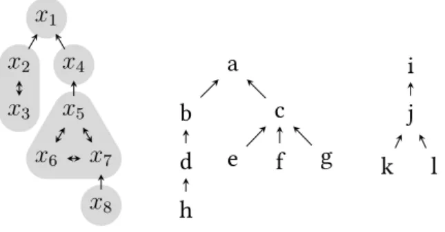
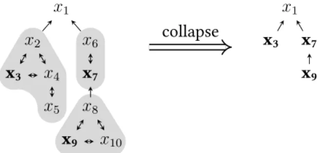
In figure 2.2 you can see a tree-quasi-ordering that is not a tree ordering, as some downward closures are not linear, e.g. in the downward closurecl(x₃)you can see that x₂ 4x₃ andx₃ 4x₂, makingcl(x₃)not a partial ordering. Later in this chapter we will see a simple method how to get a tree ordering from a tree-quasi-ordering by collapsing the strongly connected components (highlighted in gray). The root isx₁, the leaves are x₃ andx₈ and the depth is 4, because a strictly increasing sequence with maximal length isx₁ ≺x₄ ≺x₅ ≺x₈.

2 Definition of the logic

x₁ x₂ x₃

x₄ x₅ x₆ x₇

x₈

a b d h

c

e f g

i j

k l

Figure 2.2:A tree-quasi-ordering and a tree ordering

On the right you can see a tree ordering, as all downward-closures are linear. Furthermore, it is an example for a tree ordering consisting of multiple sub-trees – tree orderings can also be forests. The roots areaandi, while the leaves areh, e, f, g, kandl. The depth of this tree ordering is 4 because of the sequencea≺b ≺d≺h.

Definition 2.8(Data Words)

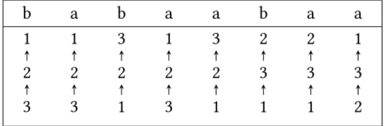
Let Σ be a finite alphabet, ∆ an infinite domain of data values and A a finite set of attributes. Then the finite sequencew= (a₁,d1)(a₂,d2)· · ·(a_n,dn) ∈(Σ×∆^A)⁺is an A-attributed data wordwith length|w|=n, consisting of tuples of lettersa_i ∈Σand data valuationsdi ∈ ∆^Awhich map each attribute to some data value. We usew_i, i ∈ [n]to denote the letter at thei-th position(a_i,di)of the word.

IfA= [k], the valuations may be called vectorsand represented ask-tuples(x₁, . . . , x_k) withx_i ∈ ∆so thatd(i) = x_i for all i ∈ [k]. If Ais a different linear ordering with k elements, it can be treated like[k], identifying each elementa∈Awith the unique size of its downward-closure|cl(a)|, which is an element of[k].

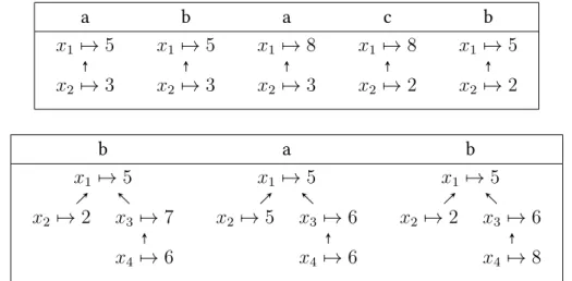
In figure 2.3 you can see two examples for data words with a common finite alphabet Σ ={a, b, c}and infinite value domain∆ = (N,=), but different sets of attributes. In the first word we have a set of attributesA₁ = {x₁, x₂}, in the second word we have A₂ ={x₁, x₂, x₃, x₄}. As you can see, in each position of the word the value assigned to any attribute can change. For example, in the first word in the second position we have a valuationd2withd2(x₁) = 5,d2(x₂) = 3, while in the next position we have a valuation d3withd3(x₁) = 8,d3(x₂) = 3.

A noteworthy aspect you can see is that in both examples the attributes exhibit a quasi- ordered structure – in the first word the setA1has the ordering relation4¹={(x1, x2)},

2.1 Preliminaries

a b a c b

x₁ 7→5 x₂ 7→3

x₁ 7→5 x₂ 7→3

x₁ 7→8 x₂ 7→3

x₁ 7→8 x₂ 7→2

x₁ 7→5 x₂ 7→2

b a b

x₁ 7→5 x₂ 7→2 x₃ 7→7

x₄ 7→6

x₁ 7→5 x₂ 7→5 x₃ 7→6

x₄ 7→6

x₁ 7→5 x₂ 7→2 x₃ 7→6

x₄ 7→8

Figure 2.3:Examples for data words

making (A₁,41) a linear ordering. In the second word the set A₂ has the relation 42={(x₁, x₂),(x₁, x₃),(x₁, x₄),(x₃, x₄)}, making(A₂,42)an example for a tree order- ing. Exactly such types of orderings for multi-attributed data words are the kind we are going to work with.

Unlike in the first word of figure 2.3, for linear-ordered attribute sets that are isomorphic to([k],≤)the attribute names in all following examples will be omitted and just addressed with a number, i.e. the smallest attribute is just called1, the second-smallest is called2 and so on, up to the maximal element addressed withk, k ∈N. The graph representation of a linear-ordered data valuation will then just contain the values associated with the corresponding attribute, without mentioning the actual attribute.

Definition 2.9(Data Valuations)

Let A be a quasi-ordered set andd,d⁰ ∈ ∆^A_⊥ some partial data valuations. d is called equivalenttod⁰(written: d'd⁰) if and only if there is a bijectionh :dom(d)→dom(d⁰) so that for alla, a⁰ ∈dom(d) :a4a⁰ ⇔h(a)4h(a⁰)∧d(a) = d⁰(h(a)).

In figure 2.4 you can see the same attribute set multiple times, each time with different subsets highlighted, denoting the attributes which are in the domain of the corresponding partial data valuation. The previous definition tells us, that two partial valuations are equivalent if the domain and ordering of both is isomorphic and the corresponding attributes hold the same values.

Althoughd1andd2are isomorphic – you can mapx2tox3 andx4tox5and have a linear

2 Definition of the logic

x₁ 7→3 x₂ 7→5 x₄ 7→1

x₃ 7→1 x₅ 7→3 x₆ 7→3 x₇ 7→3

x₈ 7→7

x₁ 7→3 x₂ 7→5 x₄ 7→1

x₃ 7→1 x₅ 7→3 x₆ 7→3 x₇ 7→3

x₈ 7→7

x₁ 7→3 x₂ 7→5 x₄ 7→1

x₃ 7→1 x₅ 7→3 x₆ 7→3 x₇ 7→3

x₈ 7→7

x1 7→3 x₂ 7→5 x₄ 7→1

x₃ 7→1 x₅ 7→3 x₆ 7→3 x₇ 7→3

x8 7→7

x1 7→3 x₂ 7→5 x₄ 7→1

x₃ 7→1 x₅ 7→3 x₆ 7→3 x₇ 7→3

x8 7→7

Figure 2.4:Examples of different partial data valuations (d₁, . . . ,d₅) of the same attribute set

ordering of size 3 in both cases – the values do not match, as5 =d1(x2)6=d2(x3) = 1 and1 = d1(x4)6=d2(x5) = 3, sod1 6'd2.

If we compared2 andd3, we see that although the number of attributes in both subsets is the same and we could map attributes with identical values to each other, this does not suffice. If we would mapx₅ tox₆ andx₃tox₄, we still would have the problem that x₃ 4 x₅, but x₄ 64 x₆, so the relation is not preserved in the mapping and therefore d2 6'd3.

When comparing e.g.d2 andd4 we already can see just from the structure thatd2 6'd4, because we can not create a bijection between two subsets with different size.

Finally, for a positive example, we can conclude thatd4 'd5, because we can mapx₆ to x₇and have in both cases a linear order of size 4 and also the corresponding values are the same – trivially for the shared attributes and becaused4(x₆) = d5(x₇) = 3.

2.2 Syntax and semantics

2.2 Syntax and semantics

Now we have all the pieces that we need to construct our logic:

Definition 2.10(Syntax)

Let Abe some finite set of attributes andAP a finite set of atomic propositions,p ∈AP andx∈A.

The following grammar describes syntactically valid formulae inLTL^↓_A[X,U,∃≥,∀^x_≤]:

ϕ ::= p | ¬ψ | ϕ∧ϕ | ϕ∨ϕ

| Xϕ | ϕUϕ | ↓^xϕ | ↑^x

| ∃≥ϕ | ∀^x_≤,ψϕ

ψ ::= p | ¬ψ | ψ∧ψ | ψ∨ψ

| Xψ | ψUψ | ↓^x ψ | ↑^x

Parentheses may be used freely to represent the structure of a formula.

Definition 2.11(Syntactic sugar)

The following additional operators are regarded as syntactic sugar and can be used when appropriate:

true := p∨ ¬p p∈AP false := ¬true

ϕ⇒ψ := ¬ϕ∨ψ ϕ⇔ψ := (ϕ⇒ψ)∧(ψ ⇒ϕ) Fϕ := trueUϕ Gϕ := ¬F¬ϕ

Xϕ := ¬X¬ϕ ϕRψ := ¬(¬ϕU¬ψ)

The definition 2.10 provides a minimal set of common LTL operators, as you can get most familiar operators from well-known equivalences defined in 2.11, which use the minimal set of operations to define everything else. By choosing this path, the core syntax is kept small and easy to handle, while still allowing us to use convenience operators to make formulae more readable.

Definition 2.12(Semantics)

Let(A,4)be a finite tree-quasi-ordered set of attributes,AP a finite set of atomic proposi- tions andΣ =P(AP)a finite alphabet encoding subsets ofAP,w= (a₁,d1). . .(a_n,dn)∈

2 Definition of the logic

(Σ×∆^A)⁺a data word of lengthn ≥1,d∈∆^A_⊥a partial data valuation,i∈[n]a position inwandx∈A.

The following satisfaction relation inductively defines the semantics ofLTL^↓_A[X,U,∃≥,∀^x_≤]: (w, i,d)|= p :⇔ p∈a_i

(w, i,d)|= ¬ϕ :⇔ (w, i,d)6|=ϕ

(w, i,d)|= ϕ∧ψ :⇔ (w, i,d)|=ϕand(w, i,d)|=ψ (w, i,d)|= ϕ∨ψ :⇔ (w, i,d)|=ϕor(w, i,d)|=ψ (w, i,d)|= Xϕ :⇔ i+ 1 ≤nand(w, i+ 1,d)|=ϕ

(w, i,d)|= ϕUψ :⇔ ∃i≤k≤n : (w, k,d)|=ψ and∀i≤j<k : (w, j,d)|=ϕ (w, i,d)|= ↓^x ϕ :⇔ (w, i,di|_cl(x))|=ϕ

(w, i,d)|= ↑^x ϕ :⇔ ∃y∈A :di|_cl(x) 'd|_cl(y)

(w, i,d)|= ∃≥ϕ :⇔ ∃_d⁰∈∆^A,x∈A: (w, i,d⁰|_cl(x))|=ϕ

(w, i,d)|= ∀^x_≤,ψϕ :⇔ ∀j≤i : (w, j,dj)|=ψ ⇒(w, i,dj|_cl(x))|=ϕ

Notice, that our storing capability is limited – we can not store and compare arbitrary attributes by themselves, but only downward-closures of an attribute, or put in a different way, we can only store complete paths from an attribute to a root element and compare them to other paths. So we can only compare attributes together with all other “ancestor”

attributes they depend on.

We gain a bit of flexibility from the definition of the check-operator↑^x, as we can also compare non-isomorphic paths. This is possible, if we previously stored an attribute with a downward-closure with a bigger size and then check an attribute with a downward-closure with a smaller size. Explained visually, we can store an attribute at some deep position in the tree and then check an attribute in a higher position. The check-operator can just ignore the additional values, as it looks for a compatible, isomorphic downward-closure.

Obviously this does not work in the other direction, though, as we can not extend our closure afterwards in any meaningful way. So storing a less deep attribute and checking a deeper attribute afterwards will always fail.

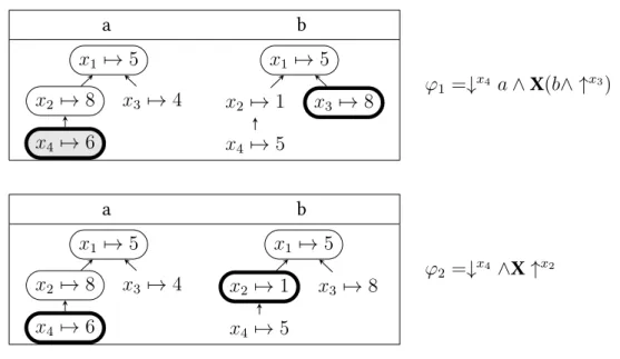
For illustration, consider figure 2.5. The formulaϕ1 checks thataholds in the first posi- tion and at the same time stores the downward-closure of the attributex4. In the next

2.2 Syntax and semantics

a b

x₁ 7→5 x₂ 7→8 x₄ 7→6

x₃ 7→4

x₁ 7→5 x₂ 7→1 x4 7→5

x₃ 7→8 ϕ₁ =↓^x4 a∧X(b∧ ↑^x3)

a b

x₁ 7→5 x₂ 7→8 x₄ 7→6

x₃ 7→4

x₁ 7→5 x₂ 7→1 x₄ 7→5

x₃ 7→8 ϕ₂ =↓^x4 ∧X↑^x2

Figure 2.5:An example usage of the “forgetful” check operator

1 2 3 4 5 6

c a c a b c

x1

5

x2

8 x4

6 x3

4

x1

5

x2

1

x4

5 x3

4

x1

5

x2

4 x4

5 x3

4

x1

5

x2

4

x4

9 x3

4

x1

3

x2

7 x4

3 x3

3

x1

5

x2

4

x4

3 x3

3

ϕ=F(b∧ ∀^x_≤,a³ X↑^x2)

Figure 2.6:An example usage of the∀^x_≤,ψoperator

position it checks thatbholds and compares the stored values to the downward-closure of the attributex₃. The formula is satisfied, as the check restricts the downward-closure of the stored attribute to x₁ andx₂, ignoring x₄ and getting an isomorphic linear or- dering that can be compared and indeed has the same values. In ϕ₂ on the contrary, there is no restriction of the downward-closure of x₄ that has the same values as the downward-closure ofx₂, so the formula is not satisfied.

For the sake of simplicity, in all examples the alphabet that is used in data words is assumed to encode sets that contain just a single proposition with the same symbol as the letter, so when you see anain a data word, it really means the set containing the propositiona, that is{a}.

2 Definition of the logic

b a b a a b a a

1 2 3

1 2 3

3 2 1

1 2 3

3 2 1

2 3 1

2 3 1

1 3 2

ϕ=∃≥((b⇒ ¬ ↑³)U(a∧ ↑³))

Figure 2.7:An example usage of the∃_≥operator

The∃≥-quantifier allows us to guess and store an arbitrary attribute with an arbitrary data value in the register and check that the following sub-formula is satisfied. This can be used to express the notion that there exists some valuation in the future for which some property holds. The∀^x_≤,ψ-quantifier allows us to express that the following sub-formula should be satisfied for all valuations of an attributexup to the current position, for all positions whereψ held. Theψ constraint is required for the linearisation which will be described later and allows us to filter the set of positions to be quantified over. If no filtering is desired, theψcan be just set to true. In that case, theψ may be omitted completely, so that∀^x_≤denotes∀^x_≤,true. Also, for linear orderings thexparameter can be omitted, because there is no ambiguity with regard to the branch to be stored (as there is only one) and the correct depth can be obtained by the automatic restriction of↑^x, as described above.

In figure 2.6 you can see the∀^x_≤,ψoperator in action — the formula checks that finallyb holds and then checks, that the data value stored forx3in all previous positions wherea held is the same as the value stored inx2in the next position. For the given data word this is indeed the case —aheld in positions 2 and 4, so these positions are quantified over. bholds finally in position 5 and the values ofd2 andd4restricted tox3are indeed the same as the valued6restricted tox2.

In figure 2.7 the formula says that there exists a position wherea holds and that the value ofx₃ at that position is never seen at previous positions at whichbheld. This is a translation of the example given in Figueira (2012) of a property that can not be expressed without the∃_≥ operator. You can verify that the formula is satisfied by observing that the valuation in the last position of the word is never used before. Now it is clear how the logic defined in this chapter works, but we have yet to prove that it is decidable. For this proof we first need the automata model presented in the next chapter.

3 Nested Register Automata

In this chapter I will present the automata model that is used in the next chapter to prove decidability of LTL^↓_A[X,U,∃≥,∀^x_≤]. The automata are a generalization of alternating register automata (ARA) as defined in (Figueira, 2012, Def. 3.1), adjusted to work with ordered data. I will extend this automata model with the two opearations guess and spreadfrom Figueira (2012) that were originally missing in the generalization, but are required for the translation of∃≥and∀^x_≤operators in the next chapter.

Next, I will present necessary terminology from the framework ofwell-structured transi- tion systems, which was introduced in Finkel and Schnoebelen (2001) as a generalization of multiple notions, with the aim to simplify and unify the concepts required to prove decidability in different contexts.

Finally I will present a proof by Decker and Thoma¹that emptiness is decidable for NRA, which is based on this framework. The proof originally did not include the necessary cases for guessandspread, so I will consider these cases where it is relevant, thereby adapting it to NRA that include these two additional operations.

3.1 Definition of NRA

Thek-NRA automaton we will define now is a nondeterministic one-way automaton that can be thought of having a set of synchronized threads, working independently, with the restriction that all threads move to the next position of the word simultaniously. Each thread has a register, having the ability to store the data vector of a position and check the saved value for equality at some later point.

We will extend it with the capability to guess an arbitrary data value withguessand use spreadto create new threads for each already existing thread in some specific state.

1private communication

3 Nested Register Automata

As our automata will run on finite data words and will be able to see just one position at a time, it is desireble to know when we have reached the end. The following definition offers us a clean way to express this information:

Definition 3.1

Letw∈(Σ×∆^A)⁺be a data word with|w|=n. Lettype_w(i) : [n]→ {., .}be theword typeofw, mapping each position of the word to a symbol indicating whether there is a next position in the word:∀_i∈[n−1] :type_w(i) =.,type_w(n) =..

Usingtypewe can access this metainformation for some word and position in the states of our automata and.will indicate that we are at the end of the word. In the next chapter we will need this to correctly encode the weak next operatorXfrom some formula into a NRA.

Definition 3.2(k-NRA)

LetΣ =P(AP)be a finite alphabet encoding subsets of atomic propositionsAP,Qa finite set of states,q₁ the initial state,k ∈ Nthe maximum register depth andδ : Q → Φ a transition function from states to expressions defined by the grammar

ϕ:=p|p| ?|store(q)|eq_i |eq_i |q∧q⁰ |q∨q⁰ |.q|guess(q)|spread(q, q⁰) withp∈AP, q, q⁰ ∈Q, ∈ {., .}, i∈[k].

The tupleA= (Σ, k, Q, q₁, δ)is called analternating k-nested register automaton (NRA).

Letw∈(Σ×∆^[k])⁺,|w|=nbe a[k]-attributed data word of lengthn≥1.

AconfigurationofAis a tuple(i, α, γ, T), wherei∈ [n]denotes the position inw,α = type_w(i)is the word type of the current position, γ = wi is the current input letter and T ∈ P<∞(∆^[k]×Q)is the set of activethreads, where a single thread(d, q)∈T consists of a vector of data values d stored in its register and its current state q. The set of all configurations of ak-NRA is denoted withC_NRA^k .

A stateq∈Qis called moving, ifδ(q) = .q⁰ for someq⁰ ∈Qand a configuration is called moving, if for all(d, q)∈T the stateqis moving.

Letρ= (i, α,(a,d),(d⁰, q)∪T)be a configuration. Thenon-moving transition relation

→⊆ C_NRA^k × C_NRA^k is defined as follows:

3.1 Definition of NRA

ρ→ (i, α,(a,d),{(d⁰, q_i)} ∪T) :⇔δ(q) =q₁∨q₂, i∈ {1,2}

ρ→ (i, α,(a,d),{(d⁰, q₁),(d⁰, q₂)} ∪T) :⇔δ(q) =q₁∧q₂ ρ→ (i, α,(a,d),{(d, q⁰)} ∪T) :⇔δ(q) =store(q⁰)

ρ→ (i, α,(a,d), T) :⇔δ(q) =eq_i and∀1≤j≤i :d(j) = d⁰(j) ρ→ (i, α,(a,d), T) :⇔δ(q) =eqi and∃1≤j≤i :d(j)6=d⁰(j) ρ→ (i, α,(a,d), T) :⇔δ(q) =β? andα =β, β ∈ {., .}

ρ→ (i, α,(a,d), T) :⇔δ(q) =pandp∈a ρ→ (i, α,(a,d), T) :⇔δ(q) =pandp6∈a ρ→ (i, α,(a,d),{(e, q⁰)} ∪T) :⇔δ(q) =guess(q⁰),e∈∆^[k]

ρ→ (i, α,(a,d),{(d⁰⁰, q₁)|(d⁰⁰, q₂)∈T} ∪T) :⇔δ(q) =spread(q₂, q₁)and(∗)

(∗): For spread(. . .) it is demanded, that all other possible → transitions are already executed, in order to take into account all new data values that were possibly introduced in these transitions.

The moving transition relation→.is defined as:

(i, ., γ, T)→_. (i+ 1, α⁰, γ⁰, T⁰)

with α⁰ = type_w(i + 1), γ⁰ = wi+1, T⁰ = {(d, q⁰) | (d, q) ∈ T, δ(q) = .q⁰} iff the configuration(i, ., γ, T)is moving.

Finally, we define thetransition relationbetween the configurations as→:=→ ∪ →_.. Arun on a data wordw ∈ (Σ×∆^[k])⁺ is a non-empty sequenceC₁ → . . . → C_nwith C₁ = (1, α₁, γ₁,{d₁, q₁}). A run isaccepting, iffC_n = (i, α, γ,∅)contains an empty set of threads. If for an automatonAthere is some wordw ∈ (Σ×∆^[k])^∗ for whichAhas an accepting run, we say thatAisnon-empty.

You can see in the definition of the transition relation that the different kinds of expressions can be classified in different groups. Some of themintroducenew threads, like ∧and spread. For example, in the case of∧both subformulae must be satisfied, so two threads are created to take care of each.

Some expressionsmodify a thread in some way, e.g. in the case of∨, the next state is nondeterministically chosen from two given possibilities, in the case ofguessthe thread

3 Nested Register Automata

A= ({a, b},3,{q1, . . . , q8}, q1, δ)

qi 1 2 3 4 5 6 7 8

δ(q_i) q₂∧q₃ a .q₄ store(q₅) .q₆ q₇∧q₈ b eq₂

w=

a a b

4 5 7

5 1 2

5 1 9 Figure 3.1:Example of a 3-NRA and an accepted word

nondeterministically saves a new vector in the register and continues the evaluation. So there can only be an accepting run over a word, if one of these choices leads to success, allowing these threads to terminate.

Some expressionseliminatethreads. This happens by definition only, if the according expression is successful, e.g. a thread witheqionly can be eliminated, if the comparison of the data vector stored in the thread and the vector at the current position of the word is successful. If this is not the case, this thread can not be removed, therefore the configuration can never become moving and the automaton can not continue to read the word.

A run always begins from an initial thread with an initial state at the beginning of the word. In each position threads are introduced, modified or eliminated, first evaluating all threads of non-moving expressions exceptspread, then thespreadoperation, which depends on the other threads and therefore waits for them to include all candidates.

Finally, when all threads in the current position are at a.-expression (the configuration is moving), the threads move on to the next position of the word. This goes on until no more transition is possible.

Directly from this transition semantics naturally comes the definition of an accepting run – if a run over a word stops, because there are no more threads, it means that we successfully checked all properties encoded in the states, ultimately leading to the termination of all threads. If a run ends with some threads still present in the configuration, it means that some assumption did not hold for the word, leaving the automaton in a stuck state, unable to continue because of no more applicable transition.

In figure 3.1 you can see an NRA with 8 states depicted in tabular form. When the automa- ton starts the run onw, it is in the configurationC1 = (1, .,(a,(4,5,7)),{((4,5,7), q1)}).

Due to the associated expressionδ(q1)the initial thread gets replaced with two threads {((4,5,7), q2),((4,5,7), q3)}. The expression ofq2 checks thataholds, which is true, so

3.2 Emptiness of NRA

this thread gets eliminated. Now the configuration is moving and so the expression of q₃ moves the thread to the next position of the word, changing to stateq₄. Next, due to thestorethe thread saves the vector(5,1,2)of the current position into the register and changes state toq₅. Again, we are in a moving state and as this is the only action left to do, the thread moves to the next position and changes into the stateq₆. Now the thread again gets replaced with two new threads{((5,1,2), q₇),((5,1,2), q₈)}. The thread in stateq₇ verifies thatbholds, becoming successfully eliminated. The last thread that is left is in stateq₈ and also gets eliminated after successfully verifying that the first two values of the vector(5,1,9)at the current position are equal to the first two values of the stored vector. Now we are left with no threads, therefore the automaton halts, accepting the wordw.

As you can easily see, the automaton discussed above represents the LTL^↓_[k] formula ϕ=a∧X↓² X(b∧ ↑²). In the next chapter a general way will be presented to translate arbitraryLTL^↓_[k][X,U,∃≥,∀^x_≤] formulae intok-NRA, so that the set of accepted words of the automaton exactly characterizes the models of the underlying formulae. But first we need to establish the fact that is is possible to verify whether a given NRA will accept anything at all, i.e. that the emptiness problem is decidable, as we need this property to show the decidability ofLTL^↓_A[X,U,∃≥,∀^x_≤] in the next chapter.

3.2 Emptiness of NRA

3.2.1 Preliminaries

The general idea of the upcoming proof is as follows. First we will show that the possible configurations of our automaton can be seen as awell-quasi-ordering, which is an ordering fulfilling some good properties. As a NRA configuration is quite complex, this will be done in multiple steps building upon each other, relying on known results from order theory. Then we will show that the transition relation of the automaton and the well-quasi-ordering harmonize in a certain way, making the configuration graph of NRA awell-structured transition system. Using this fact we will be able to imply that emptiness must be decidable, by applying an according result from Finkel and Schnoebelen (2001).

Before we can start, let us formalize these concepts:

3 Nested Register Automata

Definition 3.3(Well-Quasi-Ordering (WQO)) Let(M,4)be a quasi-ordering.

(M,4)is calledwell-quasi-ordering, if every infinite sequence of elementsm₁m₂m₃· · · from M contains two elementsm_i, m_j, so thatm_i 4m_j andi < j.

The definition of a well-quasi-ordering basically says, that it is not possible to construct infinite strictly decreasing sequences or infiniteantichains – sequences of incomparable elements.

Consider the partial ordering of natural numbers(N,≤). This is an example of a well- quasi-ordering, because starting at any numbern ∈ N, there are only finitely many numbers smaller thann, so it is impossible to create an infinite sequence that is strictly decreasing all the time – we can start the sequence decrementingnone by one, but even- tually we reach the minimal element1and then we can not go down anymore.

Now consider the partial ordering of whole numbers(Z,≤)– if we start counting down, we will never run out of smaller numbers, because there is no minimal element we will ever run into. So the whole numbers are notwell-founded and therefore(Z,≤)is not a well-quasi-ordering. Also the ordering(N,|)is not a well-quasi-ordering, where|is the divisibility relation – we know that there are infinitely many prime numbers, none of them being the divisor of any other, so the sequence of prime numbers would give us an infinite antichain.

Lemma 3.4(Erdös & Rado)

Let≤be a well-quasi-ordering. Then any infinite sequence contains an infinite increasing subsequencexi0 ≤xi1 ≤. . .withi0 < i1 < . . ..

Proof.See (Finkel and Schnoebelen, 2001, Lemma 2.2)

This fact is just a simple consequence from the definition of well-quasi-orderings – as decreasing elements are finite, at some point they are exhausted. Therefore, regardless of the element we start with, an increasing element must be taken after a finite amount of decreasing elements in between.

3.2 Emptiness of NRA

Lemma 3.5(Dickson)

Let≤_k⊆N^k0 ×N^k0 be a product ordering, i.e. such that

(x₁, . . . , x_k)≤_k (y₁, . . . , y_k) :⇔ ∀i∈[k] :x_i ≤y_i

For allk ∈N0,(N^k0,≤_k)is a well-quasi-ordering.

Proof. See Dickson (1913).

Dicksons lemma basically says that in every subset of k-tuples of natural numbers there exists a finite set of minimal elements with regard to the described ordering, thereby ensuring that no infinitely decreasing sequence in such subsets is possible, giving us a well-quasi-ordering. Originally, this lemma was used by Dickson to prove a number-theoretic statement about perfect numbers, but the statement holds for other product orderings based on well-quasi-ordered elements as well.

Definition 3.6(Embedding ordering)

Let(S,4)be a quasi-ordering andx=x₁. . . x_n, y =y₁. . . y_m ∈ S^∗, n, m∈Nbe finite sequences of elements of S. The relationv ⊆S^∗×S^∗, such that

xvy:⇔ ∃1≤i₁<...<in≤m ∀_j∈[n] :x_j 4y_ij

is called the embedding orderingoverS^∗. Lemma 3.7(Higman)

Let(S,4)be a well-quasi-ordering andv ⊆S^∗×S^∗be the embedding ordering overS^∗. Then(S^∗,v)is a well-quasi-ordering.

Proof. See Higman (1952).

Lemma 3.8(Finite Multiset WQO)

Let(S,4)be a WQO. (M(S),4^M)is called thefinite multiset WQOof(S,4)and is a WQO for4^Msuch that for all finite multisetsM ={m₁, . . . , m_p}, M⁰ ={m⁰₁, . . . , m⁰_r} ∈ M(S), m_i, m⁰_j ∈S :

3 Nested Register Automata

M 4^MM⁰ iff there is an injectionh: [p]→[r]such that∀1≤i≤p :m_i 4m⁰_h(i) Proof. From each finite multiset from M = {m₁, . . . , m_n} ∈ M(S)it is possible to construct a finite sequence of the elementsX = x₁x₂. . . x_n ∈ S^∗ by linearising the multisets in an arbitrary order using a bijectionb : [n] → [n]with b(i) = j such that m_i = x_j, mapping each element of the multiset to a position in the corresponding sequence.

Now consider an infinite sequence of multisetsM₁M₂. . . , M_i ∈ M(S). For each such se- quence letX₁X₂. . . , X_i ∈S^∗be the corresponding infinite sequence of finite sequences, where eachX_icorresponds to a multisetM_iby such a bijectionb_i. From Higmans Lemma (3.7) we know, that the embedding ordering over finite sequences(S^∗,v)is a well-quasi- ordering, therefore in every such infinite sequence there are someX_i, X_jso thatX_i vX_j andi < j, which means that for eachx_k ∈X_ithere is somex_l ∈X_j, such thatx_k 4x_l. Let p = |X_i|, q = |X_j|. By construction, we know that each x_k corresponds to a uniquem_f(k) in the according multiset M_i and each x_l corresponds to a uniquem_g(l) in the multisetM_j by some bijectionsf andg. Therefore we have for allk ∈ [p]that m_f(k) 4 m_g(l) for somel ∈[q]. We can easily construct an injectionh: [p]→[q]with h(f(k)) = g(l), making sure thatm_r 4 m_h(r) for allr ∈ [p] and therefore have by definitionM_i 4^M M_j. We conclude, that(M(S),4^M)is also a well-quasi-ordering.

The embedding ordering is a construction on top of sequences of quasi-ordered sets, for example, we can define the embedding ordering over finite sequences of natural numbers.

In figure 3.2 you can see that there is a subsequence ofy so that each element ofxis smaller than the corresponding element of the subsequence ofy, soxvy. In the case ofz you can not find a subsequence ofythat fulfills that condition, we would have to start at the3which is trivially smaller or equal than the3inz, but then we have not enough positions inyto find corresponding elements to eachz_i, soz 6vy. As we have to match every position of the left sequence to positions of the right sequence, which is not possible if the left sequence is longer, it is clear thaty6vxandy 6vz and that in general this relation can only be symmetrical in cases where both sequences have the same length. Higmans lemma tells us, that such embedding orderings are always also well-quasi-orderings, if the underlying ordering is a well-quasi-ordering.

3.2 Emptiness of NRA

x= 2 1 5

v ≤ ≤ ≤

y= 1 2 3 4 5

6w ≥ ≥ ≥

z= 3 4 2 1

x=

2, 1, 5

4 M ≤ ≤ ≤

y=

1, 2, 3, 4, 5

< M ≥ ≥ ≥ ≥ z=

1, 2, 3, 4 Figure 3.2:Comparison with embedding orderingvover(N^∗,≤)

and finite multiset ordering4^Mover(M(N),≤)

If you remove the information about positions from some sequence, you get a set contain- ing all these elements in an arbitrary order, possibly containing duplicates – a multiset.

In the upcoming proofs a well-quasi-ordering on multisets is sufficient and sequencing is not required, so Lemma 3.8 applies Higman’s Lemma to multisets, removing the structure imposed by the sequencing. In figure 3.2 you can see, that the same values as in the embedding order, when interpreted as a multiset, can be reordered and permit more ways to compare elements. Therefore the multiset ordering is more liberal than the embedding order.

Definition 3.9(Transition systems)

LetSbe a set of states and→ ⊆ S×Sbe a transition relation. Then(S,→)is atransition system.

• Succ(s)denotes the set of direct successors andPred(s)the set of direct predcessors of states∈S.

• If Succ(s)is finite for alls∈S, the transition system is finitely branching.

• If Succ(s)is computable for alls∈S, the transition system is effective.

• A transition system with a well-quasi-order relation≤⊂ S×Sis called reflexive downward compatible with regard to≤, if and only if for alla1, a2, a⁰₁ ∈ S with a1 →a2anda⁰₁ ≤a1 there existsa⁰₂ witha⁰₂ ≤a2and eithera⁰₁ →a⁰₂ ora⁰₁ =a⁰₂. The notion of a transition system is a concept unifying different constructions that use a kind of states and transitions between them, regardless of the additional structure, like initial and accepting states, labels and other details specific to the construction. This way it is possible to talk about the behaviour and properties of different systems using the same language. In our case, the configurations of the NRA automaton from the

3 Nested Register Automata

C = (i, α,(a,d), T), T ={((4,3,2), q₀),((4,3,6), q₂),((4,1,9), q₁), . . .} ∈P₃

T =

















 4 3 2 q₀

4 3 6 q₂

4 1 9 q₁

6 1 9 q₁

6 7 4 q₅



















=



















4 3 2 q₀

6 q₂

1 9 q₁

6 1 9 q₁

7 4 q₅



















={(d₁, t₁),(d₂, t₂)} d_i ∈∆, t_i ∈P₂

. . .={(4,{(3,{(2, q0),(6, q2)}),(1,{(9, q1)})}),(6,{(1,{(9, q1)}),(7,{(4, q5)})})}

Figure 3.3:Forest representation of the threads of a 3-NRA configuration

previous chapter yield the transition system that we will talk about. Now, to show that emptiness is decidable, the main task is to prove that NRA configurations give rise to a well-quasi-ordering and their transition relation is reflexive downward compatible with regard to their well-quasi-ordering, making NRA awell-structured transition system.

3.2.2 Proof of decidability

Definition 3.10(Thread forests)

LetPk:=P≤∞(∆^[k]×Q), k >0denote the set of finite subsets of[k]-attributed NRA-threads andP0 :=P(Q).

An element T ∈ P_k can be viewed as a forest and represented as a set of tuples {(d₁, t₁), . . . ,(d_n, t_n)}, where d_i ∈ ∆ are the roots and t_i ∈ P_k−1 are the sets of cor- responding subtrees. Letsub(T) = {t₁, . . . , t_n}denote the multiset of sets of subtrees.

In figure 3.3 you can see how a set of NRA threads can be seen as a forest – a thread consists of a state and a valuation for the linear ordered attributes. We can build a forest out of threads using a shared data valuation prefix, because we know that the values in a linear data vector are depending on each other. This way we obtain a compact representation of all values which are present in the current configuration that we can better reason about.

Note however, that these forests haveno relation at allto the tree-quasi-ordered attributes from some possible underlyingLTL^↓_A[X,U,∃≥,∀^x_≤] formula, being based on data equality on prefixes of[k]-vectors. This notion is formalized in the following definition: