Sensor networks: Exposure problem
Baptiste Prˆ etre
Abstract
A fundemental property of sensor networks is coverage: how well a sensor network can cover a certain terrain. In general, coverage answers questions such as the quality of service provided by a sensor network and is thus a very good quantifier for sensor networks.
The exposure of an object in a sensor network depends on how well the sensor network can observe the object moving on an arbitrary path over a period of time. It is directly related to a sensor network’s coverage. The analysis of exposure thus helps us to study a sensor network’s coverage, giving us important information about the sensor network itself. Knowing the minimal exposure path is of great use. It is on this path that we should add new sensors, should we want to improve the general coverage efficiently.
We will give a brief introduction about sensor networks. After that we will discuss the exposure problem first. We will formally define exposure and it’s properties. Then we will look at the solutions presented in the papers to compute the minimal exposure path of a sensor network. Finally, a few more personal opinions will be expressed on the subject.
1 Introduction
1.1 Sensor networks
A sensor network is a computer network of many, spatially distributed devices using sensors to monitor conditions at different locations, such as temperature, sound, vibration, pressure, motion, or pollutants. Usually these devices are small and inexpensive, so that they can be produced and deployed in large numbers. Hence, their resources in terms of energy, memory, computational speed or bandwidth are severely constrained. Each device is equipped with a radio transceiver, a small microcontroller, and an energy source, usually a bat- tery [1]. A sensor network is usually connected to a gateway in order to pass on the measured data. This gateway can consist of a special sensor node or more simply a computer connected to a network.
Sensor networks are applied in a wide variety of areas, such as video surveil- lance, traffic monitoring, air traffic control, robotics, cars, home monitoring and manufacturing, and industrial automation.
1.2 Motivation
There has recently been renewed interest in wireless sensor networks. Rapid progress was achieved in computation and communication technology as well as the emerging new low-cost, more reliable MEMS-based sensors. This gave the means to meet the increasing demands of applications that can observe and even influence the physical world.
In addition to the new applications, wireless sensor networks offer an interesting alternative to several existing technologies. Ventilation systems in large build- ings, for example, often have many enviromental sensors hardwired together with the ventilation system. Alone the savings in the wiring costs could justify a replacement by a wireless sensor network.
1.3 Challenges
There are a few things that set sensor network protocols apart from other more classical distributed systems protocols. The communication-computation trade- off is the core idea behind low-energy sensor networks. A good algorithm de- signed for wireless sensor networks will require a minimal amount of communi- cation as communication is very energy demanding. This is in sharp contrast with classical algorithms where the goal generally is maximizing the speed of execution. This renders classical distributed algorithms ill-suited for develop- ping useful wireless sensor networks algorithms [3].
A protocol designed for sensor networks must also be very flexible as sensors can be rendered useless easily. They can be covered and thus unable to commu- nicate, they can run out of power, they can be moved or simply be physically damaged. Most sensor network algorithms thus tend to build ad-hoc networks:
they only communicate with their neighbors.
1.4 Location discovery
There is one last thing we must look at before we can tackle the real problem.
How do sensors know their location? They could be dropped on the terrain from a helicopter and must still dynamically build a network. It is not sufficient for a sensor only to know it’s neighbors. If a sensor wants to send data back to the gateway, it should send it to the neighbors nearest to the gateway instead of aimlessly flooding the network.
There are three ways for a sensor to learn it’s position:
Deterministic placement: The location of the sensor was manually en- tered. This can be done if the sensor is not randomly disposed, but deliberatly placed.
GPS: The sensor has a GPS receiver or anything it could use to find it’s position on it’s own, independently of the network or the other sensors.
Multilateration: If a sensor has three neighbors which already know their positions, it can use multilateration to deduce it’s position. Each neighbour can perceive the sensor at a certain signal strength, and can thus situate it on a certain circle. By intersecting the 3 obtained circles, the sensor can thus learn it’s position (two circles generally yield two possible locations).
In practice, usually all three methods are used. A subset of the devices have GPS or are programmed manually, then the rest learn their position by multilateration.
2 Exposure
2.1 Motivation
Why should we worry about exposure? What do we learn from studying the exposure of a sensor network? Let’s admit we have flown over a forest and dropped sensors randomly. The sensors have intialized, they have discovered their neighbors as well as their location and built a network. Surely we would know like to have an idea how efficient our sensors are. Are they well deployed or are there breaches an enemy could exploit to traverse the network undetected? If this is the case how can we add more sensors as efficiently as possible? Exposure helps us answer such questions.
The exposure of an object in a sensor network depends on how well the sensor network can observe the object moving on an arbitrary path. It is directly related to the coverage of a sensor network. In normal computer algorithms we study the worst case in order to gain information on the execution time of the algorithm. In analogy, the minimal exposure path provides valuable information about the worst case exposure-based coverage in sensor networks [2].
Knowing the minimal exposure path is of great use. If we wish to improve the coverage of a sensor network, then it won’t help a lot to add new sensors in already well covered regions. On the other hand, we can efficiently improve the coverage by adding just a few new sensors along the minimal exposure path (improving the worst case).
2.2 Matematical models
In order to be able to study the exposure problem seriously, we need to introduce it formally. Because of the many different sensor devices exisiting on the market nowadays, there exist numerous mathematical models of varying complexity.
Yet, most sensing device models share two common characteristics [2]:
• Sensing ability diminishes as distance increases.
• Due to diminishing effects of noise bursts in measurements, sensing ability can improve as the alloted sensing time increases.
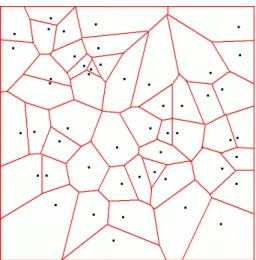
Figure 1: Voronoi diagram.
First we will introduce the Voronoi diagram and then make our way to expo- sure’s mathematical model.
2.2.1 Voronoi diagram
The Voronoi diagram is the mathematical model which impersonates the intu- ition to stay away from sensors as much as possible. In 2D, the Voronoi diagram of a set of discrete sites (points) partitions the plane into a set of convex poly- gons such that all points inside a polygon are closest to only one site (in our case, a sensor).[3] This construction effectively produces polygons with edges that are equidistant from neighboring sites.
In other words, the edges of the Voronoi diagram maximize the distance to the sensors. As we will later see, exposure is very dependent on the distance to the sensors. Constructing a minimal Voronoi-based exposure path is thus a good approximation of the minimal exposure path.
2.2.2 Sensibility
We express the general sensibility for sensorS at an arbitrary pointpas S(s, p) = λ
[d(s, p)]k
where d(s, p) is the Euclidean distance between the sensor s and the point p, and positive constants λand K are sensor technology-dependent parameters.
It is important to note here, the important role of the distance (usuallyk= 2) [2].
2.2.3 Intensity
All-Sensor Field IntensityIA(F, p) for a pointpin the fieldF is defined as the effective sensing measures at pointpfrom all sensors inF.
IA(F, p) =
n
X
i=1
S(si, p)
Closest-Sensor Field IntensityIC(F, p) for a pointpin the fieldF is defined as the sensing measure at pointpfrom the closest sensor inF, i.e. the sensor that has the smallest Euclidean distance from pointp.
IC(F, p) =S(smin, p)
Although the all-sensor field intensity is the correct one to be used, simulations often replace it with the closest sensor field intensity as it is easier to compute.
Only the sensibility of one sensor must be computed instead of all of them. As we saw earlier, a sensor on the other side of the terrain only has very little influence because of the importance the distance plays. Closest-sensor field intensity is thus a good approximation and simulations [2] showed it didn’t differ much from all-sensor field intensity [2].
2.2.4 Exposure [2]
The exposure for an object in the sensor field during the interval [t1, t2] along the pathp(t) is defined as
E(p(t), t1, t2) = Z t2
t1
I(F, p(t))
¯
¯
¯
¯ dp(t)
dt
¯
¯
¯
¯ dp
where the sensor field intensityI(F, p(t)) can either beIA(F, p(t)) orIC(F, p(t)) and
¯
¯
¯
dp(t) dt
¯
¯
¯is the element of arc length.
It is important to note that although distance plays an important role, exposure is also dependent on the time spent in the system.
2.3 A simple example
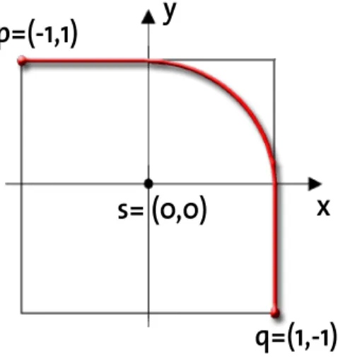
To grasp the beauty and the complexity hiding behind the apparent simplicity of the problem, it is very interesting to consider the following example. We simply ask ourselves what the minimal exposure path fromp= (−1,1) toq= (1,−1) is, if a sensor is placed at (0,0).
Our first intuition would be to try to stay as far away from the sensor as possible (following the Voronoi edges). Yet if we use the exposure model presented just before, we find out that the minimal exposure path makes an arc from (0,1) to (1,0) [2]. The problem with our first intuition is that, although the distance to the sensor is maximized, we need more time to reachq. Hence, it is sometimes
Figure 2: Exposure example
For those interested in more details, there is a complete analysis of the problem in the paper of Seaphan Meguerdichian on exposure in wireless ad-hoc sensor networks [2].
3 Algorithms
In this section, we will present existing algorithms used to calculate the minimal exposure path of a sensor network. These algorithms can be seperated into two categories: those using a global knowledge of the network graph and those which only use local knowledge.
3.1 Global knowledge
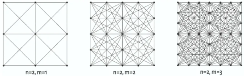
Global knowledge algorithms are slightly boring as their use is for theoretical purpose only (i.e. simulating a sensor network on a computer). The only al- gorithm presented in the papers first generates a grid over the terrain. It then computes for each edge the exposure experienced by an object if it were to travel along this edge. These steps are done to discretise the problem: the finer the grid, the more accurate the result will be. Then, using Dijkstras Single-Source- Shortest-Path algorithm, it calculates the minimal exposure path considering the the edge’s exposure as the weight (each edge is assigned a weight in Djik- stra’s algorithm).
I personally find this algorithm unelegant. It has the merit of being easy to explain and works. But in the end it is simply a brute-force approach and shouldn’t scale well. For example no use is made of the Voronoi approximation.
We could first compute the best Voronoi-based path, then discretise more ac- curatly the region around it.
Figure 3: Global knowledge, grid creation.
Of course, it is maybe not worthwhile to make a state of the art program in the global knowledge category.
3.2 Local knowledge
Local knowledge algorithms are the algorithms which are used in practice. These algorithms only need local position to work, in fact they only require each node to know his approximate position as well as his neighbors.
As mentionned before, one must keep in mind that a good sensor network pro- tocol is not necessarily the one with the best response time. Power consumption minimisation is far more important.
3.2.1 Flooding
It is interesting to note, that the author of the paper which presented this al- gorithm is also the author of the global knowledge algorithm. Both algorithms apply the same basic idea, only a few additional mechanisms must be added in order to make it work with only local knowledge. The general idea works as fol- lows, interested readers should consult the paper [4] for additional information.
• The path request query generated by an agent contains the initial location I and the destination D. This query is initially received and handled by the node closest to I. The node then builds the initial Exposure Profile for each boundary edge and sends updates with the corresponding exposure profiles. It then behaves no differently than any other node.
• Upon receiving an update order for the first time, each node computes it’s Voronoi cell (it knows it’s position as well as it’s neighbors position).
It then calculates all exposure profiles based on the profiles it has just received. These exposure profiles consist of the point-to-point exposures along the boundary edges of the node’s Voronoi cell. It then forwards updates to all it’s neighbors with the corresponding exposure profiles (the exposure profile of the edge the neighbor has in common).
• If a node receives further update orders, it checks if it’s current profiles need to be updated. An update is needed if the received exposures are smaller than the ones he already has. If this is the case, the node updates it’s profiles and sends an update to all it’s neighbors with the updated profiles. If the update is unnecessary, the sensor sends an ”abort update”
back to the sender. This is only a tool to prevent unnecessary updates from flooding the whole network.
• Once a node computes the exposure to the destination D it broadcasts the result in a ”dest update” message. The algorithm is done once all nodes terminate their search and report back to the initiating node.
These mechanisms implement a distributed version of Dijkstras Single-Source- Shortest-Path algorithm whilst it is left to each node to compute it’s edge ex- posure profile (local discretisation). It is clear that this algorithm shares the same approach as the general knowledge algorithm.
3.2.2 Greedy
This protocol is much more adapted to sensor networks as fewer messages are exchanged (thus reducing power consumption). Once again, each sensor com- putes it’s Voronoi cell and the sensor nearest to the initial location handles the query. The algorithm then keeps choosing the most ”interesting” neighboring cell from the set of all unvisited cells. ”Interesting” is not only chosen on the weakest cell exposure, but the distance to the destination also plays a role. A message is then sent to the sensor in this ”interesting” cell, which computes a discretisation of it’s cell’s exposure. It sends the result back to the origin. When the message reaches the origin, it is possible to compute the minimal exposure experienced to reach this ”interesting cell”. The minimal exposure path is thus updated and the cell marked as visited. The algorithm then computes the new most ”interesting” sensor and continues. The algorithm stops once a sensor has reached the destination with it’s cell.
An accurate description of the algorithm is in paper[5].
3.2.3 Other possiblities?
There are many other programming techniques which can be applied to com- pute the minimal exposure path. Flooding and greedy are only two possible approaches. One could also try simulated annealing, swarm or even genetic al- gorithms.
It would be interesting to compare state-of-the art algorithms programmed each using a different technique not only on the minimal exposure path found, but also on the number of exchanged messages.
4 Conclusion
The minimal exposure path in a sensor network is it’s worst case. Once a sensor network deployed, it tells us what minimal exposure an enemy must withstand in order to pass unnoticed. If the exposure level is too small, then additional sensors must be added on the path until the exposure level is satisfying. Pa- per [6] studies in detail the effects of deploying a few additional sensors on the minimal exposure path. Paper [3] studies the effects on the maximum breach path, which is related to the minimal exposure path (maximum breach path be- ing the path which maximizes the distance to the sensors). Both papers come to the conclusion, that only few additional sensors must be added in order to obtain high improvements. The improvements decrease linearly as the number of sensors set up at the beginning increases.
The most considerable drawback in this subject is the difficulty to bridge be- tween the physical and theoretical world. As mentionned before, each sensor has unique characterestics which vary even more when deployed in a natural enviroment. The mathemaical models we saw allow the use of parameters, but this is not enough to accuratly model the real world’s complexity. Eventhough the theory treated in the papers is very thorough and complete, it may be the case that it is of theoretical use only and that in practice, one must resort to actual testing of the sensor network in order to find the minimal exposure path. In order to be able to apply this theory, one must find a way to accuratly mathematicaly model the real-life sensors.
References
[1] http://en.wikipedia.org/wiki/Sensor Networks [2] Exposure in Wireless Ad-hoc Sensor Networks
Seapahn Meguerdichian1, Farinaz Koushanfar, Gang Qu, Miodrag Potkon- jak
International Conference on Mobile Computing and Networking, 2001 [3] Coverage problems in Wireless Ad-hoc Sensor Networks
Seapahn Meguerdichian, Farinaz Koushanfar, Miodrag Potkonjak, Mani B.
Srivastava
International Conference on Mobile Computing and Networking, April 2001 [4] Localized Algorithms In Wireless Ad-Hoc Networks: Location Discovery
And Sensor Exposure
Seapahn Meguerdichian, Sasa Slijepcevic, Vahag Karayan, Miodrag Potkon- jak
International Symposium on Mobile Ad Hoc Networking & Computing, 2001 [5] Minimal and Maximal Exposure Path Algorithms for Wireless Embedded
Sensor Networks
Proceedings of the 1st international conference on Embedded networked sen- sor systems, November 2003
[6] Sensor Deployment Strategy for Detection of Targets Traversing a Region Thomas Clouqueur, Veradej Phipatanasuphorn, Parameswaran Ra- manathan, Kewal K. Saluja
Mobile Networks and Applications, 2003