Gate-defined coupled quantum dots in topological insulators
Christian Ertler, Martin Raith, and Jaroslav Fabian
Institute for Theoretical Physics, University of Regensburg, 93040 Regensburg, Germany (Received 8 October 2013; published 25 February 2014)
We consider electrostatically coupled quantum dots in topological insulators, otherwise confined and gapped by a magnetic texture. By numerically solving the (2+1) Dirac equation for the wave packet dynamics, we extract the energy spectrum of the coupled dots as a function of bias-controlled coupling and an external perpendicular magnetic field. We show that the tunneling energy can be controlled to a large extent by the electrostatic barrier potential. Particularly interesting is the coupling via Klein tunneling through a resonant valence state of the barrier.
The effective three-level system nicely maps to a model Hamiltonian, from which we extract the Klein coupling between the confined conduction and valence dots levels. For large enough magnetic fields Klein tunneling can be completely blocked due to the enhanced localization of the degenerate Landau levels formed in the quantum dots.
DOI:10.1103/PhysRevB.89.075432 PACS number(s): 73.63.Kv,75.75.−c,73.20.At In topological insulators (TIs), according to the bulk-
boundary correspondence principle [1,2], topologically pro- tected surface states are formed, which are robust against time- reversal (TR) elastic perturbations. In the long-wavelength limit the two-dimensional (2D) electron states at the surfaces of three-dimensional (3D) TIs can be described as massless Dirac electrons with the peculiar property that the spin is locked to the momentum, thereby forming a helical electron gas. Charge and spin properties become strongly intertwined, opening new opportunities for spintronic [3,4] applications [5–10].
To build functional nanostructures, such as quantum dots (QDs) or quantum point contacts, additional confinement of the Dirac electrons is needed. However, conventional electrostatic confinement in a massless Dirac system is ineffective due to Klein (interband) tunneling. In graphene this problem could be overcome by either mechanically cutting or etching QD islands out of graphene flakes [11–13]
or by inducing a gap by an underlying substrate, which breaks the pseudospin symmetry [14,15]. Another promising idea to overcome the restrictions given by Klein tunneling is to use graphene strips or nanoribbons. An electrostatic confinement in such a system has been proposed in Ref. [16] by employing the transversal electron motion. Moreover, an effective spin exchange coupling of two gate-defined quantum dots becomes possible in a graphene nanoribbon by indirectly coupling the dots via the tunneling to a common continuum of delocalized states [17].
In TIs a mass gap can be created by breaking the TR symmetry at the surface by applying a magnetic field. This could be achieved by proximity to a magnetic material [18,19], or by coating the surface randomly with magnetic impurities [20–22]. By modifying the magnetic texture of the deposited magnetic film, a spatially inhomogeneous mass term is induced, opening the possibility to define quantum dot (QD) regions [23], or waveguides formed along the magnetic domain wall regions [24]. Another interesting, possibly more feasible way of defining confinement regions, is to induce a uniform mass gap and to define the QDs by electrostatic gates, which are energetically shifting the band gap [25,26]. In this paper we will focus on such gate-defined topological insulator quantum dots.
Single QDs confining Dirac electrons have been thoroughly investigated in the past few years either by numerically solving tight-binding models or be deducing analytical solutions if a cylindrical symmetry and infinite-mass boundary conditions are present [27]. However, the properties of coupled QDs are much less understood and call for a detailed, inevitably numerical study. Recently we investigated coupled graphene QDs of small radii (R <30 nm) utilizing the Green’s function method to calculate the energy spectra [28]. The graphene dots have been modeled by a tight-binding Hamiltonian, since for very small dots the usage of an effective field model becomes already questionable. We obtain that, beside the strong influence of the boundary for etched graphene dots, the main difference to TI quantum dots lies in the valley degeneracy unavoidably present in graphene but not at a single- sided topological surface. For instance, if one investigates the spin precession of an Dirac electron in a single QD according to an applied perpendicular magnetic field, in topological insulators the total angular momentum, as the sum of the orbital and spin momentum (Jz=lz+sz), is conserved due to [H,Jz]=0. This leads to a dynamic transformation between orbital and a spin angular momentum during the precession in a single TI dot, which does not occur in graphene, since the valley degeneracy exactly cancels out this effect.
In this paper we investigate how an electrostatically tunable coupling strength between the TI dots of typical size of about R=50 nm and an applied external magnetic field influence the energy spectra of the double-dot system. The tunneling time is deduced from studying the wave packet dynamics, which needs the numerical solution of the time-dependent (2+1) Dirac equation. For this purpose we use a specially developed discretization scheme, which was introduced and discussed in detail in Ref. [29]. We study two different scenarios for inducing a coupling between the dots: (i) by conventional means, i.e., by electrostatically reducing the barrier height in between the dots, and (ii) by coupling the dots via Klein tunneling upon a hole state in the barrier, which can be shifted by a gate voltage. Especially in the second case we find a strong tunability of the coupling strength. We also introduce toy one-dimensional (1D) models to study tunneling of Dirac electrons analytically. Our numerical solutions for coupled
2D quantum dots establish quantitatively strong and efficient coupling between the dots. In the Klein tunneling regime we provide a useful three-level parametric hopping Hamiltonian to describe the conduction and valence band couplings. Our goal is to provide the single-electron picture of the tunneling, which could also be used as a starting point to investigate the Coulomb blockade physics.
Our paper is organized as follows. The basic idea of a gate- controlled coupling between QDs and qualitative analytical solutions are introduced in Sec.I. The numerical investigation of coupled QDs is presented and discussed in Sec.II. Summary and conclusions are given in Sec.III.
I. 1D MODEL OF A GATE CONFINED QUANTUM DOT If a uniform mass gap exists throughout the TI surface, QDs can be defined by shifting the energy gap locally by applying gate voltages as illustrated in Fig.1. The mass barrier height between the dots becomes electrostatically controllable, allowing for a direct tunability of the coupling strength. The barrier can also be shifted upwards in energy as far as a hole state comes into resonance with the ground state of the isolated dots. This leads to an effective strong coupling between the dots via Klein tunneling from the electron states to the hole state, as illustrated in Fig.2.
In order to understand qualitatively how the coupling strength between QDs depends on the barrier height, we first investigate the transmission probability of a model 1D-mass barrier. We consider two different cases: (i) a mass barrier between leads with zero mass, as illustrated in Fig.3(a), and (ii) a uniform mass gap in the structure with a shiftable region in the middle, as shown in Fig.3(b), which directly corresponds to the “conventional” coupling scenario of Fig.1.
For a general 1D structure with an inhomogeneous mass termm(x) and potentialV(x) the Dirac-Hamiltonian is
H = −iα∂xσx+m(x)σz+V(x), (1) where α=vf and σx,z denote the Pauli matrices. Let us assume that we can divide the region of interest into subregions
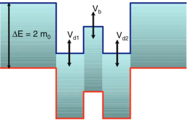
Vb
Vd1 Vd2 ΔE = 2 m0
FIG. 1. (Color online) Schematic band profile of the conduction (blue line) and valence (red line) bands of two coupled topological insulator quantum dots. The uniform band gapE=2m0is shifted by applying gate voltages. For electrons a double-dot system is formed with the barrier height being controllable by an external bias Vb. This is conventional coupling as found in semiconductor quantum dots [30].
Vb ΔE = 2 m0
FIG. 2. (Color online) Schematic band profile of the conduction (blue line) and valence band (red line) for the Klein-tunneling scenario: The coupling between the dots is realized via the Klein tunneling upon a hole state, which can be shifted by an external gate voltageVb.
in whichmandV can be assumed to be constant. For constant m and V the eigenfunctions ψ± of left (−) and right (+) moving plane waves of energyEare given by
ψ±= 1
±γ
e±iqx, (2) with
q(V ,m)= 1 α
(E−V)2−m2 (3)
and
γ(V ,m)=
(E−V)2−m2
(E+V)+m , (4)
yielding the general solution ψ=c+ψ++c−ψ−. At the boundary of neighboring subregions i and i+1 the wave function has to be continuous, resulting in the condition
ψi(xi)=ψi+1(xi). (5) This continuous connection of the wave functions of the subregions allows us to calculate the transfer matrixMof the whole system, which connects the amplitudes of the first layer
m0
d Vb
d Vb
(a) (b) (c)
FIG. 3. (Color online) (a) Scheme of a single mass barrier of heightm0. A mass barrier (b) or a quantum well (c) of widthd is formed for electrons by applying a gate voltageVb of opposite sign.
C1=(c+1,c−1) with the last, i.e., the most right oneCN =MC1. From the elements of the transfer matrix the transmission function can then be obtained by
T(E)= detM
|M22|2. (6) Mass barrier between massless dots.In the case (i) of a single mass barrier of heightm0, which is shifted by the gate voltageVb this procedure yields the following result for the transmission function if the electron energies are below the barrier, i.e.,−m0+Vb < E < m0+Vb:
T(E)= −1+6 ˜γb2−γ˜b4+(1+γ˜b2)2cosh(2dq˜b)
8 ˜γb2 , (7)
with q˜b= −iqb, γ˜b= −iγb, γb=γ(Vb,m0), and qb= q(Vb,m0). For energies above the barrier, i.e., forE > m0+Vb
andE <−m0+Vb, the transmission probability is given by T(E)=
cos2(dqb)+
1+γb22
sin2(dqb) 4γb2
−1
. (8) As expected one obtains an exponential and oscillatory dependence of the transmission function for energies smaller and greater than the barrier height, respectively, as illustrated in Fig.4. Applying a gate voltage allows one to shift the whole transmission function along the energy axis, which means that for a given fixed energy one obtains an exponential dependence on the applied gate voltage. Note that in contrast to Schr¨odinger particles the transmission remains finite even at zero energy due to the finite group velocity forE=0:
T(E=0)= cosh2 dm0
vf −1
≈e−
2dm0
vf . (9)
Uniform mass with a gate-controlled barrier.In the case (ii) of a uniform mass region m=m0 and a gate induced single mass barrier of height Vb, as shown in Fig.3(b), the transmission function results in
T(E)= 8γl2γb2 γl4+6γl2γb2+γb4−
γl2−γb22
cos(2dqb) (10) if the electron’s energy is higher than the barrier (E>m0+Vb) withγl=√
E2−m20/(E+m0). For electron energies lower
−0.3 −0.2 −0.10 0 0.1 0.2 0.3 0.2
0.4 0.6 0.8 1
E (eV)
T
Vb
FIG. 4. (Color online) Calculated transmission functionT(E) of a single 1D-mass barrier, as shown in Fig.3(a). Applying a voltageVb
allows to shiftT(E) along the energy axis, which strongly changes the transmission for a fixed energy.
0.050 0.1 0.15 0.2 0.25 0.2
0.4 0.6 0.8 1
E (eV)
T
Vb = 10 meV Vb = 30 meV Vb = 50 meV Vb = 100 meV
FIG. 5. Calculated transmission functionT(E) of a gate induced 1D barrier of widthd=30 nm, as illustrated in Fig.3(b), for different applied biases. The mass is set tom0=50 meV.
than the barrierm0< E < m0+Vbthe transmission is given by
T(E)= 1
4 3+cosh(2dq˜b)+γl4+γ˜b4sinh2(dq˜b) γl2γ˜b2
−1
. (11) Again one obtains an exponential and oscillatory dependence of the transmission function for energies below and above the barrier height, as illustrated in Fig.5for different barrier heights.
Energy spectrum of 1D TI dots.Finally, we calculate the energy spectrum of a single dot of widthd, as illustrated in Fig.3(c). By using the condition detM=0 the eigenenergies of the bounded states are given by
En= ±
nπ α d
2
+m20+Vb. (12)
II. COUPLED 2D DOTS
A. Numerical solution of the time-dependent 2D Dirac equation Here we provide a numerical investigation of the spectrum of two coupled topological insulator two-dimensional quan- tum dots depending on their coupling strength and external perpendicular magnetic fields B. In order to calculate the energy spectra we study the dynamics of wave packets (see Ref. [31] for a review of the wave packet method in general).
In comparison to a direct numerical diagonalization of the Hamiltonian, the wave packet method allows us to investigate larger systems with a higher number of grid points in a reasonable computation time. This is needed since the dot systems have to be large enough to make an effective theory actually applicable for describing the carrier dynamics of dot systems. The energy spectrum is then obtained by a Fourier transformation of the wave packet autocorrelation function with the energy resolution being determined by the total propagation timeE=2π/T. However, as a disadvantage compared to exact diagonalization the wave packet method can miss some eigenenergy values in the case that the corresponding amplitudes of the Fourier transformation are smaller than the numerical signal noise.
In order to obtain the energy spectrum we calculate the local density of states
D(E,r)= −1
πIm[G(r,r;E)], (13) which is defined via the diagonal elements of the re- tarded Green’s function G(E). Based on the dynamics of a single wave packet initially centered at r the retarded Green’s function can be constructed from its autocorrelation functionC(t),
G(r,r;E)≈ 1 i
∞
0
dt eiEt/C(t), (14) with
C(t)=
drψ(r,0)∗ψ(r,t). (15) Equation (14) becomes exact for aδ-distributed initial state, whereas in the numerical simulations a Gaussian shaped initial state is used [31]. To obtain the correlation function one has to keep track of the wave packet transient, which requires the solution of the time dependent 2D-Dirac equation
∂ψ(r,t)
∂t =HDψ(r,t). (16) The single-particle Hamiltonian at the surface of TIs can be derived within an effective field theory approach [1,2], yielding
HD =vf{[−i∇−eA(r,t)]×zˆ}σ+mz(r)σz−eφ(r,t), (17) whereA(r,t) andφ(r,t) denotes the space- and time-dependent vector and electrostatic potential, respectively. The inhomo- geneous mass term mz(r)σz is induced by breaking the TR symmetry at the TI surface, e.g., by proximity of a magnetic layer [18,19] or by magnetic doping [20–22]. The order of magnitude for the mass-gapgap=2|mz|can be expected to be tens of meV.
In order to solve numerically the (2+1) Dirac equation we use a specially developed staggered-grid leap frog scheme, which we introduced and discussed in detail in Ref. [29].
The numerical solution of the Dirac equation on a finite grid is a more subtle issue than for the nonrelativistic Schr¨odinger equation. As well known from lattice field theory, discretization of the Dirac equation leads to the so-called fermion-doubling problem, i.e., for large wave vectors a wrong energy dispersion is revealed. This leads to the doubling of the eigenstates at a fixed energy value. For a longtime propagation it is of great importance to use an almost dispersion-preserving finite-difference scheme, since scattering at spatiotemporal potentials and at the boundary can introduce higher wave vector components even when one starts with a wave packet with its wave vector components closely centered at k=0.
Moreover, the formulation of proper boundary conditions is crucial to avoid spurious reflections and eventually instability [29].
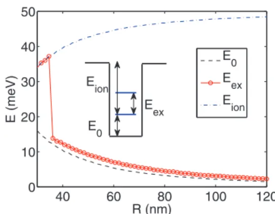
40 60 80 100 120
0 10 20 30 40 50
R (nm)
E (meV)
E0 Eex Eion Eex
Eion
E0
FIG. 6. (Color online) The ground state energyE0 (solid line), the excitation energyEex (dashed line), and the ionization energy Eion (dash-dotted line) of single dot for different radii R at zero magnetic field.
B. Energy spectra of single and coupled QDs 1. Energy spectra of single QDs
First, we investigate the confinement energy of a single isolated QD as a function of radiusRand the magnetic fieldB.
The circular dot potentialφd(r0) centered atr0is assumed to be described by the Fermi-Dirac function
φd(r0)=Vdφ˜d(r0)=VdFD(r0−r), (18) with FD(x)=[1+exp(x/βr)]−1; Vd denotes the potential height. The potential step is smeared on the range ofβr = 0.01R. In the following we set the Fermi velocity to vf = 105 m/s and the dot potential height is chosen as |Vd| = 50 meV. Figure6shows the ground state or confinement energy E0 of the dot, the excitation energy defined as difference of the ground and first excited dot stateEex=E1−E0, and the ionization energyEion= |Vd| −E1, as given by the energy difference of the ground state energy to the continuum of the delocalized states, as a function of different dot radii at zero magnetic field. For radii smaller than aboutR <38 nm only a single bound state exists in the QD and, hence,Eex=Eion. As expected, the weaker confinement of the Dirac electrons in larger dot systems leads to a decreasing of both the ground state energyE0and the excitation energyEex, as shown in Fig.6. For small radius (here forR <35 nm) only a single energy level is present and, hence, the ionization energy and the excitation energy coincide. For increasing dot radius more energy levels emerge successively. However, the steep slope of the in principle continuous line of the confinement energy cannot be resolved by our used grid of the radiusRand appears therefore as a kink in Fig.6. Note that the typical confinement energy of Dirac electrons is of the order of 10 meV, which is an order of magnitude higher than in conventional semiconductor dots of comparable size. The energy spectrum for the lowest QD levels versus magnetic field, which is applied perpendicular to the TI surface, is plotted in Fig.7assuming a fixed radius of R=50 nm. A detailed analytical study of the energy spectrum of a single graphene quantum dot in a perpendicular magnetic field is given in Ref. [27]. The eigenspectrum of the dot for
0 1 2 3 4 0
10 20 30 40 50
B (T)
E (meV)
FIG. 7. Magnetic field (B) dependent energy spectrum of a single QD of radiusR=50 nm. The energy levels converge to Landau levels for higherBfields.
B=0 is obtained by solving the implicit equation
Jm(kR)=Jm+1(kR), (19) withJmdenoting the Bessel functions of first kind of orderm and E=vfk. Since the total angular momentum Jz= lz+(/2)σz, withlzdenoting the orbital momentum operator, commutes with the Hamiltonian ([H,Jz]=0), m is a good quantum number. Hence, the ground state withl=0 is doubly degenerate according to its spin. For higher magnetic fields the levels start to converge to degenerate Landau levels, which are determined by the expression [27]
Em=vf
2eB(m+1). (20)
As can be seen in Fig. 7 at about B≈3.6 T the first two levels converge numerically, which leads to a sudden kink in the magnetic field dependence of the excitation energy Eex, as indicated by the solid red line in Fig.8. The magnetic field effectively acts as an additional confinement causing an almost linear enhancement of the confinement energyE0.
0 1 2 3 4
0 10 20 30 40
B (T)
E (meV)
E0
Eex
Eion
FIG. 8. (Color online) Magnetic field (B) dependence of the ground state energyE0(solid line), the excitation energyEex(dashed line), and the ionization energyEion (dash-dotted line) of single dot of radiusR=50 nm.
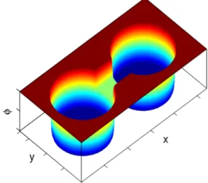
FIG. 9. (Color online) The double-dot potential in the TI surface.
The coupling of the two dots is controlled by shifting the barrier potential.
2. Energy spectra of coupled QDs
Our double-dot system comprises two circular disks, which are connected by a potential bridge, as shown in Fig. 9.
The barrier or bridge potentialφb=Vbφ˜b is described by a rectangular step function of widthwand lengthd, which is smeared at the boundaries by Fermi-Dirac function
φ˜b=FD(−w/2−y)FD(y−w/2)FD(−d−x)FD(x−d).
(21) The total potential of the coupled QD system can then be defined by
φ(r)=Vdφ˜dd+Vbmax(|φ˜b| − |φ˜dd|,0), (22) with ˜φdd =max[ ˜φd(r1),φ˜d(r2)] describing the potential of the decoupled double-dot system.
For the quantitative simulations we choose the following structure parameters: dot radius R =50 nm, bridge length d=30 nm, bridge widthw=40 nm, grid resolution x = y=1 nm, and an uniform mass term of m0=50 meV.
To ensure the stability of the discretization scheme [29] the Courant-Friedrichs-Lewy (CFL) condition has to be fulfilled t <min(x,y)/vf. We use typicallyNt=1.6×10⁵time steps for each wave packet propagation, which leads to an energy resolution of about E≈0.1 meV in the discrete fast Fourier transformation (FFT), whereE=2π/(Ntt).
The finite energy resolution of the fixed energy grid of the discrete FFT becomes noticeable in the following plots of the energy spectrum as small discontinuous jumps when external parameters, such as the barrier voltage, are changed.
The dependence of the energy spectrum on the gate- controlled barrier heightVb for B=0 is shown in Fig. 10.
ForVb =0 the two dots are almost isolated. To realize the
“conventional coupling” as illustrated in Fig. 1 a negative bias has to be applied, which reduces the barrier potential.
At aroundVb= −40 meV the bonding and antibonding states start to be split in energy bydue to the increasing coupling between the dots (Fig. 11). From the energy splitting the tunneling time follows asτ =2π/.
−100 −50 0 50 100 150
−5 0 5 10 15
Vb (meV)
E (meV)
H1 H2
Δ
Δ
FIG. 10. Calculated energy spectrum of the double TI QD system versus applied barrier gate voltage forB=0.
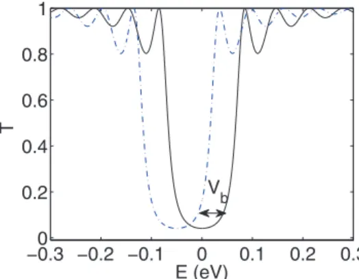
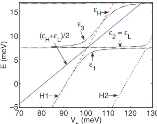
If a positive bias is applied, the hole states in the barrier region are shifted upwards in energy enabling at some point the electrons to hop by Klein tunneling from one QD to the other via the hole state, as illustrated in Fig. 2. The hybridization of the two electron levels and the hole state induces an anticrossing of the first excited electron state and the hole state, leading to a strongly tunable excitation energy of maximally≈8 meV, giving a typical tunneling time of τ ≈0.5 ps. Figure12shows this anticrossing as a zoom-in of Fig.10.
The main features of Fig. 12 can be understand by an effective three-level model. As a starting point we assume that the direct hopping between the left and right single dot ground states|Land|R, respectively, is inhibited and only hopping via the hole state|His possible. Then the effective Hamiltonian in the basis{|L,|H,|R}reads
H0=
⎛
⎝εL it 0
−it∗ εH it 0 −it∗ εL
⎞
⎠, (23)
with εR =εL, and t denotes the hopping amplitude. The eigenenergies are given by
ε2=εL, ε1/3= εL+εH
2 ∓1
2
(εL−εH)2+8t2, (24)
−100 −50 0 50 100 150
100 101
Vb (meV)
Δ (meV)
FIG. 11. Energy splittingof the first bonding and antibonding state (as extracted from Fig.10) versus the applied biasVb.
70 80 90 100 110 120 130
−5 0 5 10 15
Vb (meV)
E (meV)
H2 εH
H1
ε1 ε3
(εH+εL)/2 ε2 = εL
FIG. 12. (Color online) Zoom-in of Fig.10in the region, where the two dots are coupled via Klein tunneling upon approaching hole stateH1. An effective three-level model reveals that the anticrossing should be symmetric around (εL+εH)/2.
and the (unnormalized) eigenstates result in ϕ2(0)=(1,0,1),
(25) ϕ1/3(0) =(−1,ξ(−i∓
1+2/ξ2),1),
withξ =(εL−εH)/2t. This suggests that one eigenenergy value should remain almost unaffected and that the anticross- ing should be symmetric around (εL+εH)/2. As illustrated in Fig. 12 this behavior is approximately fulfilled by our numerical simulation results.
If one introduces an additional weak direct coupling between the dots as described by the Hamiltonian
H1=
⎛
⎝ 0 0 it1
0 0 0
−it1 0 0
⎞
⎠, (26)
perturbation theory yields that the eigenergies ofH0 are not changed in first order. However, now a small component of the hole state of the order oft1/(ε2−ε1) mixes to the eigenstate ofε2=εL:
|ϕ2 = |ϕ2(0)− 2it1
ε2−ε1|ϕ1(0)− 2it1
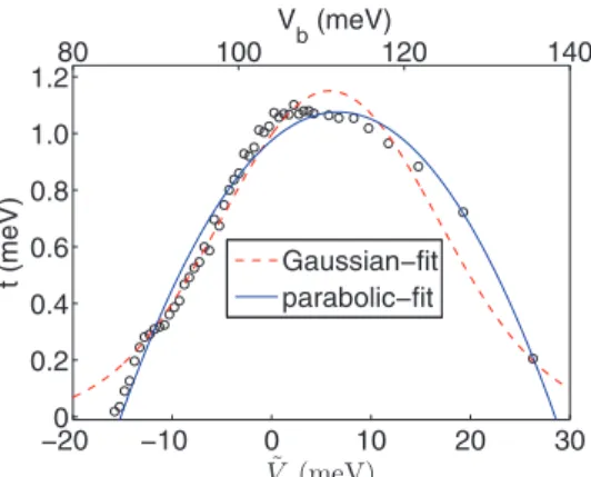
ε2−ε3|ϕ3(0). (27) From our numerical data we can extract the voltage dependence of the hopping parametert. Therefore, we redefine the origin of the coordinate system as the crossing point in which εL=εH, i.e., at the point εL=7.5 meV and V0 = 100.82 meV. ThenεL=0 by definition and the bias-dependent hole state is described by the asymptotic linear function εH(Vb)=kH(Vb−V0)=kHV˜, shown as dashed (red) line in Fig.12, withkH =0.77 being obtained by linear regression.
From the numerical results for the lowest eigenvalueε1( ˜V) we calculate the hopping parameter, which is given by
t( ˜V)=
ε12−ε1εH
2 . (28)
Figure13shows the obtained voltage dependence of the hop- ping parameter. Since the coupling between the electron and hole state vanishes for large voltages, i.e., limV˜→±∞t( ˜V)=0,
−200 −10 0 10 20 30 0.2
0.4 0.6 0.8 1.0 1.2
V˜ (meV)
t (meV) Gaussian−fit
parabolic−fit
80 100 120 140
Vb (meV)
FIG. 13. (Color online) Voltage dependence of the hopping pa- rameter t of the effective three-level model as extracted from the numerical data of the first eigenvalueε1.
we fit our numerical results to an Gaussian, as shown in Fig.13.
For comparison also a parabolic fit is provided. The effective model is most suitable in the region for ˜V between 0 and 10 meV, wheret≈1 meV is roughly constant. Otherwise the model is to be treated as a convenient parametric fit.
A qualitatively different dependence of the energy spectrum on the applied barrier biasVbis found if a strong enough mag- netic field is applied, which induces the formation of Landau levels of magnetic quantum numbersmcorresponding to the total angular momentum Jz=lz+/2σz, with lz denoting the orbital momentum. As shown in Fig.14(forB =4 T) the first hole level almost does not couple to the energy levels of the first Landau niveaus withm=0. This follows from the fact that due to theB field the states are more localized, so that their overlap, on which the hopping parameter essentially depends, is exponentially smaller. This is most pronounced for the lowest state for m=0 but can be also seen for the first excited states (m=1), where the effect of anticrossing is smaller than for the case of a vanishing magnetic field.
−10035 −50 0 50 100 150
40 45 50 55
Vb (meV)
E (meV)
H1 m = 1
m = 0
FIG. 14. (Color online) Energy spectrum of the double-dot system versus applied barrier gate voltage forB=4 T.
III. CONCLUSIONS
We have shown that the coupling between two quantum dots, which are geometrically defined by gate electrodes, can be strongly modulated and controlled by both a gate bias, which brings a hole level into resonance with the electron states, and a perpendicular magnetic field, which changes the symmetry properties of the confined states. The anticrossing of the hole state and the dot ground states can be qualitatively understood within a three-level model, in which only hopping to the hole state is assumed. The Klein-tunneling assisted coupling leads to energy splittings of the order of 10 meV, which corresponds to typical tunneling times of several hundreds of femtoseconds.
ACKNOWLEDGMENTS
This work has been supported by the German Research Foundation under the Grants No. SFB 689 and No. GRK 1570.
We thank P. Stano and R. Hammer for very valuable and fruitful discussions.
[1] M. Z. Hasan and C. L. Kane,Rev. Mod. Phys.82,3045(2010).
[2] X.-L. Qi and S.-C. Zhang,Rev. Mod. Phys.83,1057(2011).
[3] I. ˇZuti´c, J. Fabian, and S. Das Sarma,Rev. Mod. Phys.76,323 (2004).
[4] J. Fabian, A. Matos-Abiague, C. Ertler, P. Stano, and I. ˇZuti´c, Acta Phys. Slovaca57,565(2007).
[5] S. Raghu, S. B. Chung, X.-L. Qi, and S.-C. Zhang,Phys. Rev.
Lett.104,116401(2010).
[6] A. A. Burkov and D. G. Hawthorn,Phys. Rev. Lett.105,066802 (2010).
[7] I. Garate and M. Franz,Phys. Rev. Lett.104,146802(2010).
[8] O. V. Yazyev, J. E. Moore, and S. G. Louie,Phys. Rev. Lett.
105,266806(2010).
[9] T. Yokoyama, Y. Tanaka, and N. Nagaosa,Phys. Rev. B 81, 121401(2010).
[10] V. Krueckl and K. Richter,Phys. Rev. Lett.107,086803(2011).
[11] L. A. Ponomarenko, F. Schedin, M. I. Katsnelson, R. Yang, E. W. Hill, K. S. Novoselov, and A. K. Geim,Science320,356 (2008).
[12] J. Guttinger, C. Stampfer, S. Hellmuller, F. Molitor, T. Ihn, and K. Ensslin,Appl. Phys. Lett.93,212102(2008).
[13] S. Schnez, F. Molitor, C. Stampfer, J. Guttinger, I. Shorubalko, T. Ihn, and K. Ensslin, Appl. Phys. Lett. 94, 012107 (2009).
[14] G. Giovannetti, P. A. Khomyakov, G. Brocks, P. J. Kelly, and J. van den Brink,Phys. Rev. B76,073103(2007).
[15] B. Trauzettel, D. V. Bulaev, D. Loss, and G. Burkard,Nat. Phys.
3,192(2007).
[16] P. G. Silvestrov and K. B. Efetov,Phys. Rev. Lett.98,016802 (2007).
[17] M. Braun, P. R. Struck, and G. Burkard,Phys. Rev. B84,115445 (2011).
[18] L. Fu and C. L. Kane,Phys. Rev. B76,045302(2007).
[19] X.-L. Qi, T. L. Hughes, and S.-C. Zhang, Phys. Rev. B78, 195424(2008).
[20] Y. L. Chen, J.-H. Chu, J. G. Analytis, Z. K. Liu, K. Igarashi, H.-H. Kuo, X. L. Qi, S. K. Mo, R. G. Moore, D. H. Luet al., Science329,659(2010).
[21] Q. Liu, C.-X. Liu, C. Xu, X.-L. Qi, and S.-C. Zhang,Phys. Rev.
Lett.102,156603(2009).
[22] Y. S. Hor, P. Roushan, H. Beidenkopf, J. Seo, D. Qu, J. G.
Checkelsky, L. A. Wray, D. Hsieh, Y. Xia, S.-Y. Xu et al., Phys. Rev. B81,195203(2010).
[23] G. J. Ferreira and D. Loss, Phys. Rev. Lett. 111, 106802 (2013).
[24] R. Hammer, C. Ertler, and W. P¨otz, Appl. Phys. Lett. 102, 193514(2013).
[25] P. Recher, J. Nilsson, G. Burkard, and B. Trauzettel,Phys. Rev.
B79,085407(2009).
[26] G. Pal, W. Apel, and L. Schweitzer,Phys. Rev. B84,075446 (2011).
[27] S. Schnez, K. Ensslin, M. Sigrist, and T. Ihn,Phys. Rev. B78, 195427(2008).
[28] M. Raith, C. Ertler, P. Stano, M. Wimmer, and J. Fabian,Phys.
Rev. B89,085414(2014).
[29] R. Hammer and W. P¨otz,Comput. Phys. Commun. 185, 40 (2014).
[30] P. Stano and J. Fabian,Phys. Rev. B72,155410(2005).
[31] T. Kramer, E. J. Heller, and R. E. Parrott,J. Phys.: Conf. Ser.
99,012010(2008).