Construction of a user-level probabilistic forecast of electric vehicle usage

(1)

Research Collection

Student Paper

Construction of a user-level probabilistic forecast of electric vehicle usage

Author(s):

Hilpisch, Benedikt Publication Date:

2020-02

Permanent Link:

https://doi.org/10.3929/ethz-b-000460506

Rights / License:

In Copyright - Non-Commercial Use Permitted

This page was generated automatically upon download from the ETH Zurich Research Collection. For more information please consult the Terms of use.

ETH Library

(2)

Construction of a user-level probabilistic forecast of electric

vehicle usage

Semester Thesis

Institute of Cartography and Geoinformation Chair of Geoinformation Engineering

Swiss Federal Institute of Technology (ETH) Zurich

Supervision Jannik Hamper

Henry Martin

Manuel Lösch (FZI Karlsruhe) Prof. Dr. Martin Raubal

Zürich, February 2020

(3)

(4)

Electric vehicles are expected to play a crucial role in future low carbon mobility systems and it is anticipated that sales will grow significantly, both through government interventions and technological advancements [46]. While dispersion of electric vehicles is often seen as potential problem on electricity distribution system level, intelligent control of charging & discharging processes oriented on electricity spot market prices could help integrate fluctuating renewable energy sources by providing flexibility to the electricity system. Alternatively, a control could also be geared towards reduction of peak load situations in the distribution grids.

Independently of whether a control strategy based on spot market prices or aiming at avoidance of grid bottlenecks is implemented, car owners will only participate if their mobility isn’t restrained. This demands for day-ahead knowledge about individual vehicle usage to efficiently schedule recharging & discharging.

Correspondingly, goals of this thesis are forecasting when the vehicle is standing at the user’s home location the next day as well as day-ahead predictions of first departure and last arrival time and daily energy demand of the car based on historical user behavior. To this end, data of a fleet of about 100 vehicles recorded over one year is processed, briefly analyzed and then used as prediction input data.

Applying various machine learning techniques, deterministic and probabilistic forecasts on when the car stands at home are made with time resolution of 15 minutes, relevant error metrics are evaluated and results get compared with a predefined baseline model. Hereafter, different pattern recognition methods are utilized to conduct deterministic and probabilistic predictions on first departure, last arrival and daily energy consumption and outcomes are assessed. In all cases, the constructed baseline models provide well performing forecasts compared to other models. However, depending on the prediction target, they can be beaten by more complex methods.

Finally, the car fleet data at hand is utilized to quantify possible financial benefits if carrying out charging & discharging oriented on electricity spot market prices. For optimization, perfect knowledge about individual car usage and market prices is assumed. Results show a relevant potential for cost savings compared to uncontrolled charging. It is furthermore possible to generate profits from arbitrage, though this comes at cost of strongly increased vehicle battery cycling.

i

(5)

(6)

(7)

Appendix 82

A Data Description 82 A.1 Feature Descriptions Discretized 15-Minute Data . . . 82

A.2 Feature Descriptions Pre-Processed Data . . . 82

(9)

(10)

Mathematical Symbols

¯

x Sample Mean

˜

x Sample Median

s Sample Standard Deviation log Natural Logarithm

µ Expectation Value (Normal Distribution) σ Standard Deviation (Normal Distribution)

Acronyms and Abbreviations

BEV Battery Electric Vehicle

CRPS Continuous Rank Probability Score DSO Distribution System Operator EU European Union

EV Electric Vehicle LR Logistic Regression MDN Mixture Density Network MLP Multilayer Perceptron

PHEV Plug-In Hybrid Electric Vehicle PV Photovoltaic

ReLU Rectified Linear Unit RF Random Forest

RMSE Root Mean Squared Error SC Smart Charging

SOC State of Charge VPP Virtual Power Plant V2G Vehicle to Grid WS Wilson Score

vii

(11)

(12)

Introduction

1.1 Motivation

Since mass motorization took place in the 1920s in the United States and after 1950 in Europe, the car has an outstanding role in the transport sectors of Western societies.

In the United States approximately 800 vehicles per 1000 people are registered, accounting for more than 80% of passenger transport and 17% of the country’s total Greenhouse Gas Emissions [32, 33, 3]. In the European Union (EU) traveling by car is accounting for 83% of passenger-kilometers and around 15% of the total Greenhouse Gas Emissions [14, 13]. Although there might be rising shares of passenger transport via other transport modes like bus or train, car transport can be expected to stay the dominant form of transportation. For instance, a market survey conducted in 2012 by McKinsey in Germany found that 78% of the 18-to-24 year olds expect to own a car in the next ten years [15, p.10].

In the context of climate change mitigation, a fuel change from fossil fuels to renewable energy is necessary in the passenger transport sector. The most efficient way to use electricity for transportation purposes is by providing it through catenary or Lithium- Ion-Batteries to the vehicle. In comparison to a Battery Electric Vehicle (BEV), a fuel-cell car needs 2.5 times more electricity per kilometer driven, for a vehicle with an internal combustion engine powered by electricity based synthetical fuels (e-fuels) this factor increases to 5 [43, p.12].

In the EU the aspirations to support alternative fuels vary greatly, but especially Western & Northern European countries like France, the United Kingdom or Germany clearly prioritize electromobility in their national mobility plans [21, p.1]. While in Switzerland the government program "Roadmap E-Mobility 2022" aims to increase the share of BEVs & Plug-In Hybrid Electric Vehicles (PHEVs) on the newly registered cars to 15% by 2022, government policies have made China the leading market for Electric Vehicles (EVs) in terms of absolute numbers [42, 34].

Besides incentives created by national policies aiming to increase the dispersion of EVs, cost reductions, in particular in the field of Li-Ion Battery Technology, are expected to significantly contribute to increase the percentage of EV in the following years. De- loitte estimates that the market will reach a tipping point in 2022 where the cost of ownership of a BEV is on par with its internal combustion engine counterparts and

1

(13)

2 1.1. Motivation expects an EV market share of 20% on global car sales in 2030, where BEVs account for about 70% of all sold EVs [46, p.3-4]. Therefore one can expect growing sales figures of EVs in Switzerland and Western Europe as well as on a global scale.

EV owners usually charge their vehicles at home, mostly in the afternoon or evening hours when returning from work, or during the night. If assuming a share of 20% BEV on the total number of cars in Germany (47,1 Million cars [22]) with an average net battery capacity of 32 kWh, which corresponds to the battery capacity of a Volkswagen e-Golf [19], this would sum up to around 300 GWh of total net storage capacity that is regularly connected to the electricity grid for recharging. To put the numbers into perspective, in 2010 the German power system had a total of 40 GWh energy storage capacity with a power capacity of around 11 GW available [27, p.5]. The German total load profile usually moves between 50 GW and 70 GW [17].

Whereas diffusion of EV is usually regarded as major challenge for electricity distribution systems, specifically if they appear to be clustered in certain areas and show high simultaneity of uncontrolled recharging, the newly available energy storage resources in form of vehicle Li-Ion-Batteries might open up new possibilities to stabilize the electricity system and support integration of fluctuating renewable energy generation. Assuming that it is possible to remotely influence vehicle recharging, and also considering the option to discharge to the grid, different possibilities for making use of those expected future resources have been suggested in literature:

Grid-Oriented Charging refers to controlling the recharging process such that load peaks in the distribution systems due to many EVs charging in parallel are avoided and investment needs into new infrastructure on the distribution system level are reduced.

A study done for Germany found significant cost reduction potentials of 40% to 50%

for a time horizon of 2030. Participating EV owners could get reimbursed through reduced grid charges [31, p.36 & p.43-45].

Smart Charging (SC), often also called Market-Oriented Charging, shifts the charging process to time slots with low wholesale energy market prices. Electricity suppliers of EV owners could reduce their energy procurement cost and pass a part of cost savings on to their customers to incentivize participation. On the one hand, this charging control scheme could increase distribution system load as the synchronism of charging processes is likely to increase. On the other hand it would help to efficiently integrate fluctuating renewable energy sources. Power demand through charging would depend upon price signals from the day-ahead electricity spot markets which are influenced by availability of wind and Photovoltaic (PV) generation [31, p.18].

Vehicle to Grid (V2G) relates to a situation where EVs are not only taking up energy from the grid, but are also feeding electricity back into the grid. A pooling coordinator could aggregate EVs into a Virtual Power Plant (VPP) and schedule charging

& discharging with the goal to exploit price spreads on the day-ahead wholesale electricity markets. The VPP operator would share achieved profits with the EV owners to make an involvement financially attractive. Like in the case of market-oriented

(14)

charging this control strategy presumably results in high synchronism of charging &

discharging processes, that might increase stress on the distribution grids, but could help accommodate fluctuating renewable energy sources in the electricity system [44, p.203-205].

Ancillary Services, that is primary, secondary and tertiary control reserves, could potentially be provided by pooled EVs as well. By starting or stopping power infeed into the grid from the EV battery and by stopping or starting vehicle recharging, positive or negative balancing power could be offered to the electricity system. Instead of marketing flexibility provisioned by the EVs on the day-ahead electricity wholesale markets, earnings would be made on the balancing power markets. Again, increased parallelism of charging & discharging processes might be induced [44, p.185-188].

All of the four mentioned approaches share the need for knowledge about short-term user level mobility.

Although continuous intraday markets are gaining in importance, day-ahead electricity spot markets are still most significant in terms of trading volumes in the Central European region [18]. EV aggregators applying SC or V2G strategies are most likely to trade on those markets and therefore need to estimate available capacities provisioned by the managed EV fleet on day-ahead basis. The same holds for a VPP coordinator participating in European balancing energy markets where reserve capacities are auc- tioned on, inter alia, daily basis, depending on reserve type and country [1, p.11, p.33

& p.59].

Connected to market clearing of day-ahead spot markets and expected load and predicted infeed of distributed sources, Distribution System Operators (DSOs) are assumed to anticipate possible congestions in their low and medium voltage grids for the next day, and reschedule EV recharging processes in a grid-oriented charging scenario.

To not restrain mobility of their costumers, day-ahead forecasts of individual EV usage are required.

Independent of possible financial benefits originating from participating in one of the presented schemes, the EV owner needs to be sure that his or her car is sufficiently charged to meet the owner’s mobility needs. One possibility is that the user declares planned trips one or several days ahead, for example using a smartphone app, to allow the involved DSO, electricity supplier or VPP-pooling operator a scheduling of EV charging & discharging. However users might forget to enter their trips beforehand, the system would make spontaneous trips impossible and the effort needed for regularly planning and entering trips might discourage people from participation.

An ideal system would work invisible to EV owners, minimizing the times where participants are left with insufficiently charged vehicles. Ideally, the operator controlling charging & discharging of the car would know one day ahead when the car will be on a trip (i.e. when the car is not at home and the battery storage isn’t connected to the grid) and would know about the energy demand of the trips.

(15)

4 1.2. Goals & Research Questions

1.2 Goals & Research Questions

The main goal of this thesis is to explore and assess machine learning techniques capable of providing short-term user-level mobility forecasts which can be used for optimization of charging & discharging schedules of EV batteries in order to achieve different objectives (e.g. arbitrage or avoidance of grid bottlenecks) while at the same time meeting the mobility needs of the car owners. Due to the stochastic nature of individual mobility, the focus lies on probabilistic forecasting methods based on the owner’s past car usage behavior. The aim is to obtain models capable of predicting probabilities &

probability distributions which are accurately reflecting the owners mobility patterns and underlying uncertainty of individual behavior.

Additionally, possible economic profits reachable through controlling vehicle charging

& discharging taking into account day-ahead electricity spot market prices should be examined supplementary to the mobility predictions.

Concretely, this semester thesis comprises three central objectives:

• Predicting for each 15-minute interval of the next day if the car is standing at home

• Prediction of first departure and last arrival time as well as daily State of Charge (SOC) consumption for the following day

• Quantification of possible monetary benefits employing SC and V2G strategies and optimizing charging & discharging schedules under perfect knowledge of user mobility and spot market prices using data of a fleet consisting of about 100 vehicles from 1 year

With respect to the first two objectives covering mobility predictions, it is important to mention that due to market clearing times on the Central European electricity spot markets (EPEX SPOT) [18], we assumed that scheduling of charging & discharging for each day needs to take place during the course of the previous day. Thus, on the day of scheduling there is only data for the days before, but not for the complete current day available yet. To reflect this situation correctly, predictions for a day d do not consider historical data from the day before (d-1), but only from 2 or more days before.

The rest of this thesis is structured as follows:

It starts with providing an review of publications that are dealing with the subject of EV user mobility behavior, primarily associated with coordination of EV fleet charging

& discharging, in Chapter 2.

In Chapter 3, the available EV fleet data and its transformation into data sets suitable for utilization in the context of EV usage predictions and optimization of charging &

discharging schedules is described. Moreover, the most important features of the pre- pared data are presented and briefly analyzed.

Chapter 4 contains specifications of all for EV usage predictions applied model types

(16)

along with an introduction of for model evaluation relevant error metrics and base- lines.

The following Chapter 5 is covering the first main goal, that is, predicting on user level for each 15-minute time interval of the next day if the EV is parked at home or away. For forecasts used data features are detailed and results of both deterministic and probabilistic predictions are illustrated.

Chapter 6 focuses on the second main objective, which is prediction of first departure, last arrival and daily SOC consumption per EV user and for the upcoming day. Once again, firstly model input data is characterized and secondly, obtained results for deterministic as well as probabilistic predictions are reported.

The third and last main target, i.e. economic optimization of charging & discharging schedules for the given EV fleet, is treated in Chapter 7. Underlying technical assump- tions made for optimization are given and a reference scenario of uncontrolled charging is depicted. Subsequently, optimization problem formulations in connection with SC and V2G are stated and explained, followed by a portrayal of the results.

In Chapter 8 the thesis is concluded by first summarizing essential outcomes and then giving a brief outlook on possible future work linked to the topic of this project.

(17)

6 1.2. Goals & Research Questions

(18)

Literature Review

When searching for literature in the field of mobility behavior of EV users, one can find a range of publications that are covering the topic in connection with coordination of charging & discharging of an EV fleet.

In [24] a methodology for optimization of individual EV charging schedules with the aim to reach minimum recharging cost taking into account day-ahead electricity spot market prices is presented and discussed. However, the authors assume in their system architecture that predictions of individual driving patterns based on historical or statistical data are already available.

[7] investigated a scenario in which an aggregator buys needed electricity for EVs under contract at the day-ahead electricity spot markets, while at the same time using the EV fleet to provide secondary reserves (i.e. ancillary services). EVs are seen as control- lable loads during home charging allowing participation as reserve sources in upward and downward direction. Because of the assumption that EV owners provide desired SOC together with first departure time for the next day, it was identified that only for the whole fleet aggregated electrical energy requirements needed to be predicted, individual forecasts are regarded as not suitable in this context and therefore not considered. For the case study presented in [7], synthetical data for a fleet of 1000 EVs was generated based on different driver behaviors found through a survey in combination with stochastic models.

Similar to [7], article [26] examines a setting in which an EV aggregator is coordinating EV charging schedules such that recharging cost are reduced and reserve power can be offered by the fleet on balancing power markets. A stochastic optimization method is used for coordination of EV charging schedules taking into account uncertainty in EV departures. Concretely, only vehicles for commuting purposes are considered and, based on a household travel survey conducted in the United States, it is supposed that EVs are plugged in between 9 o’clock and 17 o’clock at the user’s workplace during which charging can be scheduled. From 9 o’clock on, the number of hourly from the workplace departing EVs of a fleet is assumed to follow a normal distribution. Under this assumption scenarios are created and stochastic, scenario based optimization is implemented. Once again, optimization and charging control is executed on fleet level, not on individual vehicle level.

In [16] dynamic simulation of individual mobility behavior was applied to assess avail- 7

(19)

8

able regulation power provisioned by vehicle pools with different sizes. For simulation of individual EV usage and realization of Monte Carlo simulations, probability distributions for first departure and last arrival times based on data from a mobility study done for Germany were considered and it was supposed that EV storage is only acces- sible by an VPP aggregator after the last arrival respectively before the first departure.

However, used probability distributions are based on behavior data from a large group of people, possible estimation of distributions on an individual level (i.e. EV user level) aren’t discussed.

[25] is covering what is described as "EV VPP dilemma" faced by an EV fleet owner who is renting out vehicles while at the same time using a V2G approach to actively participate on day-ahead electricity spot markets and is trying to maximize profits.

The authors are regarding the case of EV fleets positioned in large cities. EVs are not assigned to a single user or circle of persons as they are offered for renting and it is seen as virtually impossible to accurately predict when and where a single EV will be used. Thus, forecasts are not made on individual EV level, but instead aggregate EV usage predictions on city district level are conducted using a Fourier series approach to capture demand patterns.

In the context of [47], mobility on an individual level for residents of the Bay Area (California, United States) is modeled, not based on actual EV usage data, but based on mobile phone data (i.e. coordinate data). Stay points are labeled as home, work or other and mobility motifs, outlining the individual daily travel network, are derived.

Individual mobility simulations are obtained by using a probabilistic Markov model with parameters calibrated according to individual behavior. Vehicular drivers are extracted by considering vehicle usage rates from United States census data, individual mobility of EV users is probabilistically estimated using data from an Plug-in EV driver survey.

To summarize, all of the described publications either suppose that accurate predictions of individual EV usage are available ([24]), look at scenarios were aggregated forecasts are sufficient ([7] & [25]), consider very restricting settings founded on survey data ([26]), are simulating individual mobility using probability distributions derived from behavior data of a large aggregated group ([16]), or are applying probabilistic Markov chain methods with parameters adjusted based on trajectory data to model individual mobility ([47]). Publications focusing like this thesis on the individual subject, which means forecasting EV usage on individual user level under utilization of historical EV usage data, haven’t been found.

(20)

Data Description

Predictions in this thesis are based on EV usage data obtained within the scope of the SBB Green Class E-Car Pilot Project that started in 2016 and lasted until the beginning of 2018. For more than one year 143 participants have been equipped with a first class GA travelcard, a BMW i3 EV (27.2 kWh net battery capacity) and a parking space at the train station. Furthermore participants had the possibility to use Mobility Carsharing and PubliBike, a bike rental system [41].

Figure 3.1: Completeness of BMW i3 data in percent per day and EV (Day 0 is 13.11.2016) [28].

EV usage has been recorded between November 2016 and December 2017. Availability of recordings in percent per day and EV is depicted in Figure 3.1. One will notice a data collection gap between day 300 and 350, which might be explained through incomplete data delivery. Start and end dates of the recordings differ among the users

9

(21)

10 3.1. Data Preparation

due to different delivery dates of the EVs and early stopping of recordings for some users. [28, p.3-6].

In the context of this semester thesis two data sets have been used to generate necessary input data for the predictions:

The car segment data set contains data automatically recorded by the car for all users. The data set is split into distinct segments. The begin of a new segment is trig- gered by switching on or off the car engine and by starting or stopping vehicle recharging [9]. Each segment holds information on segment start- and end time, mileage, SOC of battery, total consumed energy during that segment and, originally, also coordinate data, which however has been omitted for predictions due to privacy reasons.

The is home segment data set provided by the supervisors contains segmented data on when the car stands at the user’s home. It has been derived by combining coordinate data from the car segment data set with coordinates of the users’ homes.

A new segment starts if the is home state changes, i.e. when the user leaves or reaches home with the EV. Each segment has information on segment start -and end time and is home state, which is either True or False. For 38 EVs out of 143 EVs in the data set the is home state never changes, which might be caused by wrong information on the users’ home locations. EVs with faulty is home attribute needed to be neglected for all predictions.

3.1 Data Preparation

Based on the car segment and is home segment data set, discretized 15-minute data for each EV has been derived. This discretized data was used to obtain the input data sets needed for 15-minute binary is home predictions, last arrival, first departure and daily SOC consumption predictions and for optimization of charging & discharging schedules, defined as thesis goals in section 1.2 and covered in Chapters 5, 6 and 7.

3.1.1 Data Discretization

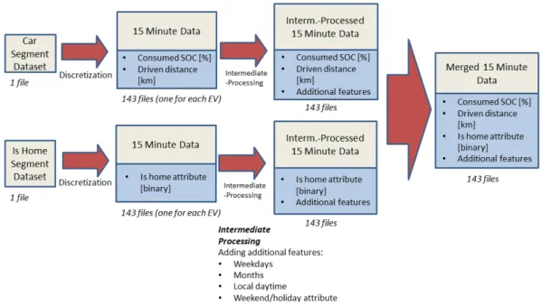
Figure 3.2 gives a schematic overview of the applied discretization procedure. Both segment data sets contain data of 143 EVs. While each of those data sets contains data for all EVs in one file, the generated discrete data is stored in separate files for each EV. A time step size of 15 minutes has been chosen as this corresponds to the smallest possible block size of energy currently traded on the EPEX Spot Markets in the Central Western Region [18].

From the car segment data set, 15-minute data on consumed SOC and driven distance is obtained. For each time step in the "grid" used for temporal data discretization, the consumed SOC and driven distance for the next 15 minutes is computed. In case a segment expands over more than one 15-minute time step the corresponding consumed SOC respectively driven distance is distributed on all intersecting time steps propor-

(22)

Figure 3.2: Schematic overview over discretization procedure.

tional to intersection time. If there is for instance a 25-minute segment with a total driven distance of 25 km of which 15 minutes lie in a first time step and the remaining 10 minutes in a second time step, 15 km are added to the driven distance of the first time step, 10 km are added for the second time step.

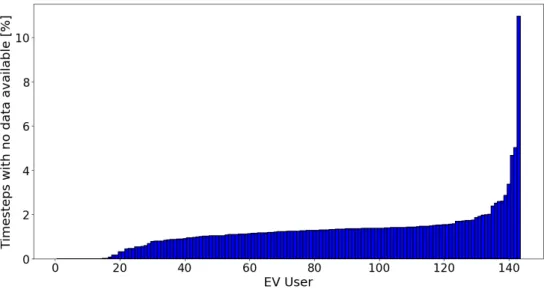
For discretization time steps lying in data recording gaps mentioned in the introduc- tory part of this chapter, driven distance and consumed SOC are set to zero. Figure 3.3 shows for each car the shares of time steps in which the car segment data set has no recordings available. One can notice that for over 90% of EVs the share of time steps with data available is above 98%. For 14 EVs the data completeness is 100 % while on the other hand a group of 9 EVs has completeness of less than 98%.

Discretization of the is home segment data set has been done such that the is home attribute is True only if the car is at home during the whole next 15 minutes, for all other cases it is set to False.

Because the time data recorded by the EV depends on the user’s setting of the car time, there might be segments for which segment end time is before or equal to segment start time. This happens if the user is changing the clock time during a segment.

Those segments have been neglected for discretization of both segment data sets.

In an intermediate processing step all discrete data sets are extended by weekday, local time, month and season features as well as by a feature indicating whether time steps lie on a working day or non-working day (i.e holiday or weekend). Finally, there are two discrete data sets for each EV which are merged into one data set for each vehicle. Figure A.1 in the appendix provides a feature list for the merged 15-minute

(23)

12 3.1. Data Preparation

Figure 3.3: Share of time steps in which no car segment data available for each EV.

discrete data with the corresponding feature explanations.

3.1.2 Data Pre-Processing for Prediction Tasks

Through a data pre-processing step, a pre-processed 15-minute data set suitable for 15-minute binary is home predictions as well as for optimization of charging & discharging schedules and a data set with daily time resolution fit for first departure, last arrival and daily SOC consumption predictions is obtained from the merged 15-minute discrete data available after the data discretization step described in section 3.1.1.

To acquire the first of those two data sets, one starts with the merged 15-minute data set at hand and adds additional features such as first departure and last arrival times and daily consumed SOC to it. Furthermore the data sets are enhanced by features indicating if the car stands at home the whole day or is away for one whole day or longer as well as by features indicating if the car is at home at the beginning (i.e.

between 0 and 0.15 o’clock) or at the end (i.e. between 23.45 and 24 o’clock) of the day. In a final step, historical features are added to make the 15-minute discrete data suitable as input foris home predictions described in Chapter 5. A detailed description of the particular input features is provided in section 5.1. A feature list for the whole pre-processed 15-minute data set can be found in Figure A.2 of the appendix.

Having the depicted pre-processed 15-minute data available, the second data set with daily time resolution is derived from the newly generated first data set and then extended by historical features to be used as input data for first departure, last arrival and daily SOC consumption predictions. A description of the prediction input data can be found in section 6.1. In Figure A.3 of the appendix a feature list for the complete daily data set is provided.

(24)

3.2 Data Inspection

As already stated in section 1.2, target variables for predictions in this semester thesis are first departure and last arrival time, as well as daily SOC consumption and the is home attribute. In the following, an overview, including a presentation and brief analysis, over these and further relevant data features is provided.

3.2.1 First Departure Time

The first departure time of the car is defined as start of the discrete 15-minute time step in which the EV user leaves home for the first time during the day. If for example the user leaves during the time step of 8.00 to 8.15 o’clock, the first departure time is set to 8.00 o’clock.

Figure 3.4: Overall data availability of first departure time.

Figure 3.4 depicts the data availability for this feature. The overall data set contains data for 143 EVs and 48650 days. However only for 11763 days (32.5 %) a first departure time is actually available. For some EVs theis homeattribute never changes (i.e. faulty is home attribute) and thus no first departure times can be computed for those users.

Additionally in cases where the car isn’t home at the beginning of the day (between 0.00 and 0.15 o’clock) or is at home the whole day, no first departure time exists.

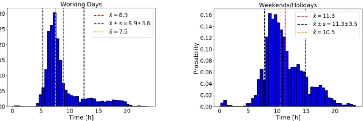
Figure 3.5 displays histograms of the first departure times of all EV users for normal working days and weekends respectively holidays. For working days there is a clear peak of first departures between 6.00 and 9.00 o’clock which can be interpreted as EV users leaving home for work. The median is 7.30 o’clock while a mean of 9.00 o’clock and standard deviation of around 3.5 hours can be reported. For weekends and holidays the median and mean of first departures are shifted forward by three hours respectively more than two hours. Owners needing the EV to get to work during the week now probably are using it for leisure or shopping activities and therefore don’t leave home that early or might not be leaving at all.

(25)

14 3.2. Data Inspection

Figure 3.5: First departure times for working days (left plot) and weekends/holidays (right plot) considering all EV users.

Figure 3.6: First departure times for working days considering two user groups: Persons who used their EV to cover more than 35 % (left plot) respectively less than 10% (right plot) of their total traveled distance.

One can look at two specific groups of EV users: The first group consists of EV users that covered more than 35 % of their total traveled distance with their EV, the second group comprises people that used it to cover less than 10% of their total traveled distance. Histograms for working days taking into account these groups of EV users are shown in Figure 3.6. The left plot considers first departure times of persons from the first group, whereas on the right data for persons of the second group is plotted. For the first group a clear peak around 7.00 o’clock can be seen, the standard deviation is reduced in comparison to the histogram for all users by around 45 minutes. In contrast to this, first departure times for persons assigned to the group of rare EV users are in general more spread out over the day and even show a small second peak in the evening hours. Compared to the data for all EV users, the sample median and standard deviation are increased by 1 hour, the mean rises by about 1.5 hours to 10.30 o’clock. This might indicate that people of the first group use their EV more regularly to get to their workplace in the morning, whereas a significant share of persons of the other group tends to use the car in the afternoon and evening hours for the first time

(26)

on a day.

3.2.2 Last Arrival Time

Figure 3.7: Overall data availability of last arrival time.

The last arrival time is defined as the end of the 15-minute time step in which the user returns home with his or her EV for the last time during a day. Figure 3.7 shows the overall availability of the last arrival time feature that is similar to the overall availability of the first departure. In addition to cases in which the car is at home for the whole day or the is home attribute is faulty, no last arrival also exists for days in which the car isn’t home at the end of the day (i.e. between 23.45 and 0.00 o’clock).

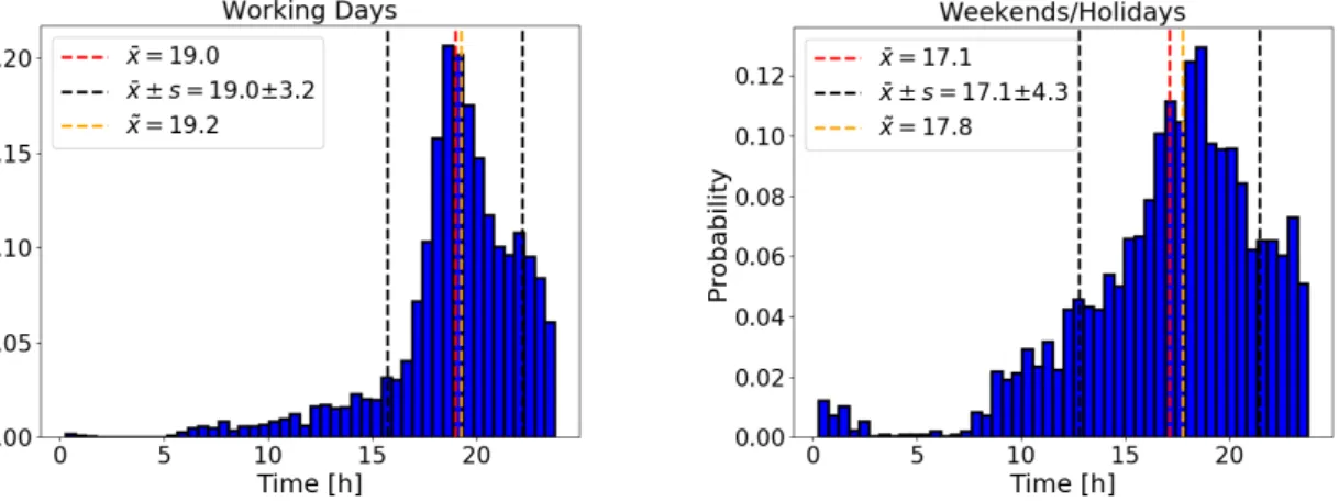
Figure 3.8: Last arrival times for working days (left plot) and weekends/holidays (right plot) considering all EV users.

Figure 3.8 presents histograms of the last arrival times for all EVs. The left plot shows last arrival times on working days, the right plot depicts them on non-working days. For

(27)

working days a peak between 18.00 and 20.00 o’clock is striking. Regarding last arrival times for holidays and weekends, one notices that compared to normal working days the mean is shifted backwards by 2 hours, the median by around 1.5 hours. Although the empirical distribution still possesses a peak in the evening hours which is observed between 17.00 and 19.00 o’clock, the sharpness of this peak is reduced. The sample standard deviation rises by 1 hour, the width of the distribution increases.

3.2.3 Daily SOC Consumption

The daily SOC consumption corresponds to the sum of SOC decreases of the vehicle battery for one entire day. If for example the owner makes a trip with the EV, the SOC will decline, the difference between SOCs at the end and beginning of the trip is negative and its absolute value (i.e. SOC consumption of the trip) will be added to the daily consumed SOC. It is important to note, that hence also through braking recuperated energy during the ride will be included.

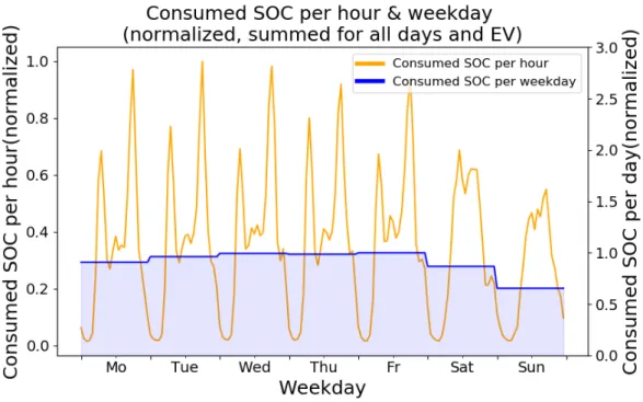
Figure 3.9: Consumed SOC per hour and per weekday summed for all days and EVs.

Figure 3.9 depicts consumed SOC per hour as well as per weekday summed and normal- ized for all days and EVs. When looking at the hourly data, two obvious consumption peaks are noticeable on weekdays, that can be interpreted as persons driving to and off their workplaces. On the weekends the peaks vanish, SOC consumption appears more spread out over the course of the day. Compared to weekdays, the overall SOC consumption is reduced on the weekends, particularly for Sundays.

A comparison between for all 143 EVs aggregated daily SOC consumption with the daily SOC consumption of single vehicles is provisioned in Figure 3.10. While the curve of aggregated daily SOC consumptions shows some form of regularity and steadiness, consumptions on single vehicle level can be described as erratic and inconsistent. This

(28)

Figure 3.10: Comparison of for all EVs aggregated daily SOC consumption with daily SOC consumption of two example cars over months August and September.

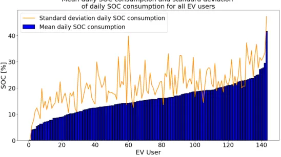
impression is confirmed when examining Figure 3.11, displaying mean daily SOC consumptions together with their standard deviations for all EV users. For the majority of EV owners, the standard deviation is larger than the mean daily consumed SOC, pointing towards high variation and randomness considering daily SOC consumption on a user level.

Figure 3.11: Mean daily SOC consumption and standard deviation of daily SOC consumption for all EV users.

(29)

3.2.4 Is Home Attribute

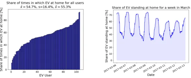
Like already mentioned in section 3.1.1, the EV is said to be at home for a given 15- minute time step only if the vehicle is standing at the user’s home location during the entire time. That being the case, the associated is home attribute is set toTrue. In the left diagram of Figure 3.12 the shares of times in which the provided BMW i3 was standing at home is presented for all users. For 18 persons it was standing at home less than 40% of the whole time, whereas for a group of 47 project participants this value is between 40% and 60%. A class of 40 people left the vehicle at home for more than 60% of the time. It is important to consider those imbalances of theis home attribute when using the data to train prediction models.

Shares of EVs located at the user’s home throughout one week in March are given in the right plot of Figure 3.12. The share of EVs at home peaks during night time, those peaks lower on the weekend, which might be caused by weekend excursions.

Furthermore one can notice, that even at night, a share of about 25 % of the vehicles is not parked at home, while a socket of around 35% of EVs remains at the user’s home location throughout the day.

Figure 3.12: Shares of times in which the EV is standing at home for each user (left) and share of EV standing at home over the course of a week in March (right). For both figures EV users with faulty is home attribute are neglected.

3.2.5 Is On Vacation Attribute

The user is said to be on vacation with his or her EV, if it isn’t at the home location during the whole day. If for example the user leaves home with the EV on Friday evening and returns on Monday morning the next week, Saturday and Sunday are marked withis on vacation attribute.

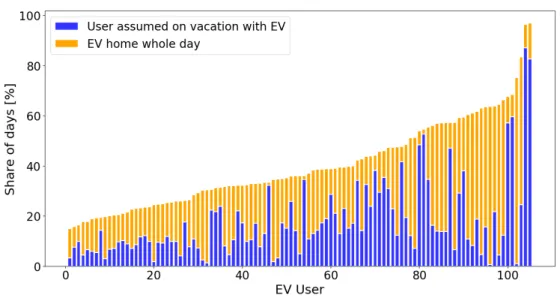
Figure 3.13 depicts the share of days for which EV users are assumed to be on vacation jointly with the share of days on which the vehicle is standing at home the whole day.

The mean share of days labeled with the is on vacation attribute is around 18% for all users, the median is at 13%. More than 70 users have been away with their EV on

(30)

Figure 3.13: Share of days on which user assumed to be on vacation with the vehicle or on which the car stands at home the whole day (for all EV users, excluding users with faulty is home attribute).

less than 20 % of the days, a small group of 8 EV owners are assumed on vacation for more than 40% of the days.

3.2.6 Is Home Whole Day Attribute

As opposed to the is on vacation feature, the is home whole day attribute marks days during which the EV continuously stands at home. This might for instance happen in cases where the user makes a journey leaving the EV at home.

In comparison to theis on vacation attribute, the mean share of days tagged with the is home whole day attribute is increased to 22%, the median rises to 18%. A group of 16 users did utilize the EV on less than 60 % of the days on which it had been available to them.

When regarding Figure 3.13 one will notice that for a large group of 40 EV users the vehicle is either standing at home or is away from the home location the whole day for over 40% of all days. This might be influenced by the pilot project setting which included possibilities for participants to use other means of transport like train or bike without additional cost, but also a reserved parking space close to the train station.

In addition, over 80 % of the participating households owned an internal combustion engine car besides the provided EV [28, p.30- 31].

Figure 3.14 is plotting the share of EVs with positive is home whole day or positive is on vacation attributes over the course of two months in spring. Remarkable are clear peaks on the weekends and holidays (here: Easter and Labor Day), since increasing number of persons might probably either stay at the home location for the entire day

(31)

or go on weekend trips.

Figure 3.14: Share of EVs which are either at home the whole day or for which the user is supposed to be on vacation with the vehicle shown over a time span of two months (excluding users with faulty is home attribute).

(32)

Methodology

In this Chapter we briefly introduce deterministic and probabilistic prediction models put to use for 15-minute binary is home predictions presented in Chapter 5 and for first departure, last arrival and daily SOC consumption forecasts discussed in Chapter 6. Furthermore, for model evaluation relevant error metrics are described.

4.1 Prediction Models

4.1.1 Is Home Predictions

In the case of theis homepredictions, only model types capable of providing both probabilistic and deterministic predictions at the same time have been considered. Thus, no differentiation into deterministic and probabilistic models is made here.

WithLogistic Regression (LR), a linear model was utilized as a first model type for is homepredictions. Model construction, training and evaluation was realized with help of the scikit-learn machine learning library (https://scikit-learn.org/stable/).

The model returns class probabilities for the is home attribute (i.e. probabilities for the attribute to beTrue orFalse), that can be directly used as probabilistic forecast or can be translated into a deterministic forecast by predicting the class with the higher probability. Classifiers were trained on the Log-loss (see equation 4.3). For regularization a L2-penalty was included, for which the respective hyper-parameter was found through a grid search.

The second used model type was a non-linear model, namely Multilayer Percep- tron (MLPs) implemented with the aid of the Keras deep learning library (https:

//keras.io/). Table 4.1 provides an overview over the model specifications. The input layer as well as all hidden layers use Rectified Linear Unit (ReLU) activation functions.The output layer consists of two units and itsSoftmax function converts values of the two numeric network outputs into probabilities. Hence, the model outputs probabilities for the is home attribute to be True or False. Those are either used directly as probabilistic forecast or are easily converted to a deterministic forecast by predicting the value with the higher probability.

21

(33)

22 4.1. Prediction Models

Table 4.1: Model specifications of used MLP for is home predictions (binary classification).

Units Activation Dropout

Input layer 256 ReLu 50%

1st Hidden Layer 512 ReLu 50%

2nd Hidden Layer 256 ReLu 45%

3rd Hidden Layer 128 ReLu 45%

Output Layer 2 Softmax -

The model was trained to minimize the categorical cross entropy loss or Log-loss (equation 4.3). Attribute imbalances in the data were taken into account by putting higher weight on losses of samples from the under-represented attribute. Weights are set in- versely proportional to the occurrence of the respective class in the data. The training data given to the model was split into a part of 75% for model fitting and 25% for estimating validation loss and error. In addition to dropout regularization, an early stopping condition was included, such that model training is stopped if the validation loss stops decreasing.

The last considered model types were Random Forest (RF) classifiers, that, like in the case of the LR classifiers, have been built using the scikit-learn machine learning library. The model implementations are based upon [10].

By taking EV data of 3 selected users and executing model fitting and evaluation for a different numbers of decision trees, a number of 250 trees has been found to be sufficient for this prediction task. Size of the random subset of features to be used for each decision tree in the random forest was determined individually for each EV data set through a hyper-parameter grid search in a range going from one to the total number of features. The model provides probabilistic forecasts by averaging the probabilistic prediction of each decision tree in the forest [40]. Again, those are converted to a deterministic forecast by predicting the attribute value with the higher probability.

Baseline

Deterministic and probabilistic predictions of the LR, MLP and RF models were compared with easy reference models.

To obtain the baseline for deterministic predictions, the most frequent is home attribute for each of the 96 15-minute time intervals in a day has been computed using all training data and is always predicted as baseline for the respective intervals. If for instance in the training data the most frequent is home attribute is True in the time interval going from 0.00 to 0.15 o’clock, i.e. for most days in the training data the EV is at home during this time, the baseline model will always predict True for this time interval in the test set. No differentiation between weekdays is made for this baseline model.

(34)

A similar approach has been applied to get the baseline of probabilistic predictions. For each of the 96 time intervals in a day, the shares of both possibleis home attributes (i.e. the shares ofTrue and False values) in the training data are estimated and predicted as probabilities for the respective time intervals in the test set. For example, if 10 % of the days in the training data contain False and 90 % contain True values as is home attribute in the time interval going from 0.00 to 0.15 o’clock, the baseline model will forecast these shares as probabilities in this time interval for all days in the test set. Again, no distinction between weekdays is made here for predictions.

4.1.2 First Departure, Last Arrival and Daily SOC Consump- tion Predictions

For all three prediction targets the same methods have been applied. Considered model types are distinguished by the type of provided prediction output, which is either a single value (i.e. deterministic) or a probability density (i.e. probabilistic).

Deterministic Predictions

The first considered deterministic model is least squares linear regression with L2- regularization, to which is often also referred to as Ridge regression. The hyperpa- rameter determining regularization strength was found by search over a logarithmically spaced parameter grid. Execution of model implementation, training and evaluation was made with the already previously mentioned scikit-learn machine learning library.

For kernelized linear regression, which is the first considered non-linear deterministic model, the linear regression method is enhanced by the kernel trick. As kernel function Gaussian radial basis functions (sometimes also called squared-exponential kernel functions) were utilized. Hyperparameters in connection with implemented L2- regularization and kernel function were obtained by a grid search. Models provided by the Scikit-learn machine learning library (that are based on [30, p.493-493]) were utilized for predictions.

As third prediction method, RF regression has been put to use. Same methodology like in case of the RF classifier used foris home predictions was applied to identify number of trees in the forest and size of random subset of features to be used for each decision tree. A number of 100 estimators was found to be adequate in this case. Mod- els and functions provided by the Scikit-learn machine learning library were used.

Lastly, MLPsproviding deterministic first departure, last arrival and daily SOC consumption forecasts were considered as additional non-linear models. Like in case of MLPs for is home predictions, networks have been built and trained with Keras deep learning library and dropout regularization as well as an early stopping condition were included to prevent overfitting. Loss function minimized during training is RMSE (see equation 4.5). A brief overview over the used MLP is given in Table 4.2.

(35)

24 4.1. Prediction Models

Table 4.2: Model specifications of used MLP for first departure, last arrival and daily SOC consumption predictions.

Output Layer 1 Linear -

Probabilistic Predictions

As first probabilistic method, linear quantile regression has been utilized. Model construction and fitting was realized with help of the statsmodels library (https:

//www.statsmodels.org/dev/index.html).

Per EV user, linear models for the 0%, 0.5%, 1%, 1.5%, ... 100% quantiles (step size of 0.5%, 201 models in total) are fitted. Thus, for each individual user there is group of quantile regression models returning forecasts on 201 quantiles of the target variable given a test sample. Interpreting model output such that probability for the forecasted variable to lie in between two adjacent quantiles is 0.5% (with the here chosen quantile step size), it can be randomly sampled from intervals between the predicted quantiles to obtain a probability density function. 500’000 random samples are drawn to estimate the related density function. It is necessary to note that linear quantile regression might output crossing quantiles. This means for instance that the model for the 1% quantile predicts a conditional quantile value of the target of 5, but the model for 1.5% quantile returns a value of 4.8 for the same test sample. For this thesis it was decided to order quantile value predictions by size for each test sample to overcome this problem. So in case of the provided example, the target value of 4.8 and 5 would simply swap places.

The second considered model type is RF quantile regression, which has been introduced by [29] in 2006. Models have been build and trained using Scikit-garden decision tree library (https://scikit-garden.github.io/). Like for the case of RF classifiers considered foris home predictions, a number of 250 trees for the models was found to be sufficient and sizes of the random subset of features to be used for each decision tree were obtained through a hyper-parameter grid search.

Probabilistic predictions are obtained in the same way already depicted in case of linear quantile regression by randomly sampling from intervals between predicted quantiles, once again using a quantile step size of 0.5% and a number of 500’000 samples. The problem of quantile crossing described in the previous paragraph for linear quantile regression hasn’t been encountered for RF quantile regression.

Additionally to the previously outlined quantile regression methods, an approach including MLPs, namelyMixture Density Networks (MDNs), which were proposed by [8] in 1994, have been tested for probabilistically predicting first departure, last

(36)

arrival and daily SOC consumption. The idea is to take a MLP which, instead of de- terministically predicting a target value, is outputting parameters of a Gaussian mixture model, comprising expectation values (µ’s), standard deviations (σ’s) and mixing coefficients of the contained Gaussian distributions. For model training, negative log- likelihood (Log-loss, see equation 4.6) is minimized.

Figure 4.1 is providing a graphical example of a general MDN model architecture.

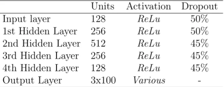
Table 4.3 is summarizing for predictions used model specifications. To offer enough flexibility in the shape of the predicted density function, it is composed of 100 Gaussain distributions. Models have been constructed with help of Keras deep learning library and a pre-built Keras MDN layer fromhttps://github.com/cpmpercussion/keras- mdn-layer.

Table 4.3: Model specifications of for first departure, last arrival and daily SOC consumption predictions utilized MDN.

4th Hidden Layer 128 ReLu 45%

Output Layer 3x100 Various -

Figure 4.1: Illustration of general MDN model architecture (source: https:

//towardsdatascience.com/a-hitchhikers-guide-to-mixture-density- networks-76b435826cca).

(37)

26 4.2. Model Evaluation & Scores

Baseline

For deterministic and probabilistic first departure, last arrival and daily SOC consumption predictions new reference models were defined.

As baseline fordeterministic predictionsthe average target values for normal working days and for non-working days (i.e. weekends or holidays) in the test data were utilized. Depending on if it is a normal working day or not, one of the two computed averages is predicted for each day in the test set.

Similarly to that, to get the baseline of probabilistic predictions, mean and standard deviation of target values in the test data, again differentiated between normal working days and non-working days, were computed. Normal distributions with distribution parameters µand σ set to the obtained mean and standard deviation values of the targets are predicted as baseline probability distributions.

4.2 Model Evaluation & Scores

4.2.1 Is Home Predictions

To assess deterministic binary is home predictions, two error metrics were taken into consideration.

The prediction accuracy reports the share of samples (i.e. 15-minute time steps) in the test set for which theis home attribute has been predicted correctly and is defined as

accuracy(y,y) =ˆ 1 n_samples

nsamples

X

i=1

1(ˆyi =yi) (4.1) where yˆ_i ∈ {0,1}(={F alse, T rue})b is the predicted is home attribute for time step i of the test set and y_i ∈ {0,1} is the actual attribute value [36].

However, for the given data, there is a non-negligible share of imbalanced data sets as for 25% of users the EV is at home either for less than 30 % or more than 70 % of the time steps (Figure 3.12).

Therefore as second metric a balanced accuracy is introduced, which is defined as balanced−accuracy(y,y) =ˆ 1

2 X

i

1(ˆy_i =y_i) P

j1(yj =yi) (4.2) where nomenclature is similar to the one in equation 4.1 [37]. The balanced accuracy measures the mean of shares of correctly classified samples for each separate class (i.e.

average of recalls on each class). In the context of the is home predictions the metric is obtained by averaging the number of correctly predicted True attributes divided through total number of True attributes and the number of correctly predicted False attributes divided through total number of False attributes. A perfect model would

(38)

have accuracy 1, a model only correctly predicting one class (e.g. a model predicting is home to beTrue for all samples) would have accuracy of 0.5 independent of number of occurrences of the two attributes in the evaluation data.

As a first metric for the evaluation of probabilistic is home forecasts theLog-losswas considered. It is defined as

L_log(y_i,pˆ_i) =−logPˆ(y_i|x_i) = −(y_ilog( ˆp_i) + (1−y_i)log(1−pˆ_i)) (4.3) wherey_i ∈ {0,1}(={F alse, T rue})b represents the actual value of theis home attribute for time step i, and pˆ_i = ˆP(y_i = 1|x_i) is the forecasted probability for it to be 1 (True) given the input features x_i [38]. This metric is the negative log-likelihood of the forecasted probability for the actual value. It is returning very large error values if the forecasted probability for the actual value is low (e.g.Pˆ(y_i|x_i) = 0.05→ L_log =

−log(0.05) ≈ 3). To obtain the overall Log-loss for a trained model, the Log-losses of all time steps i in the test set are averaged. A perfect forecasting model would have a loss of 0.

The Brier score was implemented as second metric for probabilistic forecasts. The definition is

L_Brier(y_i,pˆ_i) = (y_i−pˆ_i)² (4.4) where the same nomenclature like in equation 4.3 has been used [35]. Whereas the Log- loss penalty is logarithmic and hence strongly penalizes probability forecasts far away from the true values, the penalty of the Brier score is quadratic and thus errors are more moderate in case forecasted probabilities for the actual value are low (e.g.Pˆ(y_i|x_i) = 0.05 → L_Brier = 0.95² ≈ 0.9). The sensitivity to outliers is reduced compared to the Log-loss. Like in case of the Log-loss, the overall Brier score for a model, is computed by averaging the losses for all time steps i in the test set. An ideal model would reach a Brier score of 0.

4.2.2 First Departure, Last Arrival and Daily SOC Consump- tion Predictions

As error metric for deterministic first departure, last arrival and daily SOC consumption predictions the Root Mean Squared Error(RMSE) is considered. It corresponds to the expected value of the square root of the squared prediction error and it’s definition is written as

RM SE(y,y) =ˆ v u u t

1 n_samples

nsamples

X

i=1

(ˆy_i−y_i)² (4.5) where yˆ_i is the predicted target value for a sample i (i.e. for one day) and y_i is the actual value of the target [39]. Because the error values are squared before averaging and taking the root, the penalty isn’t linear and thus sensitive to large single errors.

(39)

To estimate the goodness of the predicted probability distributions, three error metrics measuring different aspects of quality of the predicted distributions have been reported.

The Log-loss can as well be used to analyze predicted probability distributions. Def- inition is the same like in 4.2.1:

L_log( ˆP , y_i) =−logPˆ(y_i|x_i) (4.6) In the equation, y_i represents the actual target value for sample i, and Pˆ(y_i|x_i) is the value of the forecasted probability density (given input features x_i) for y_i. In practice, Pˆ(y_i|x_i) has been computed as

Pˆ(y_i|x_i) = Z yi+

yi−

Pˆ(u|x_i)du (4.7)

where the margin around the actual value was set to 15 minutes for first departure and last arrival predictions and to 2.5 % SOC in case of daily SOC consumption predictions. For each trained model, Log-losses of test samples are averaged and reported.

Besides it’s sensitivity to outliers, a further major weakness of this score is that it evaluates estimated density functions exclusively based on their values at the actual observation [12].

Due to these shortcomings, two other metrics, which are more meaningful and eas- ier to interpret were chosen to be central for the conducted result analysis. As first additional metric the Continuous Rank Probability Score (CRPS) has been introduced. According to [23] it is specified as follows:

CRP S( ˆC, y_i) = Z +∞

−∞

C(y|xˆ _i)−H(y−y_i))²dy (4.8) C(y|xˆ i) is the cumulative distribution of the predicted probability densityPˆ(y|xi):

C(y|xˆ _i) = Z +y

−∞

Pˆ(u|x_i)du (4.9)

H(u−y_i) is the observed cumulative distribution where H(z) =

(0 for z <0

1 for z>0 (4.10)

is the Heaviside function. Figure 4.2 depicts an example for a predicted probability distribution Pˆ(y|x_i) together with the actual observation y_i on the left. The related cumulative distributions are plotted on the right. One can recognize, that the CRPS measures the difference between the predicted and actually occurred cumulative distribution functions and thus takes into account the entire shape of the predicted density

(40)

function. The goal is to achieve a low CRPS score, a perfect deterministic forecast would result in CRPS of zero. The score has the same dimension as the target [23].

Once again the scores are averaged over the test set cases for each trained model.

Figure 4.2: In the left plot an example for a predicted density together with the actual target observation is shown. In the right graph the associated predicted and occurred cumulative distributions are plotted (source: [12]).

The Wilson Score (WS) [45] is used to evaluate density predictions in terms of an acceptable range and represents the share of forecasted probability that lies within a defined tolerated margin around the observation [12]:

W S( ˆP , y_i) =

Z yi+∆y

yi−∆y

Pˆ(u|x_i)du (4.11)

The same nomenclature has been used like for equation 4.6. The tolerated distance from the actual target value y_i is denoted as ∆y and has been set to 30 minutes for first departure and last arrival time predictions and to 5% SOC in case of daily SOC consumption predictions.

Figure 4.3 shows an example for a predicted probability density Pˆ(y|x_i) including actual observation y_i and for computation of WS relevant range y_i ±∆y. The WS corresponds to the area under the estimated density in the tolerated range and can thus be interpreted as probability. The goal is to accomplish high scores, an ideal model would reach a WS of one. To obtain the WS for a trained model, scores of all test points are averaged.

The metric is sensitive to distance and the spread of the forecasts. A main weakness is the influence of the modality of the predicted distribution on the score [12].

(41)

Figure 4.3: Example for an estimated probability density together with the actual target observation and the acceptable range for the WS (source: [12]).

(42)

Is Home Predictions

The first prediction task consisted of forecasting the is home attribute on a user level for all 15-minute time steps of the next day, i.e. forecasting when the EV is standing at the user’s home, where it might be connected to the grid over the home charging point, making a control of charging & discharging possible. Moreover it was hoped to learn more about regularity of EV usage as prediction accuracy for people with regular behavior patterns is expected to be better than for people with a more erratic EV usage behavior.

In section 4.1.1 introduced predictions methods, namely Logistic Regression (LR), Multilayer Perceptrons (MLPs) and Random Forests (RFs) have been applied and compared for this binary classification task. All model types provide deterministic as well as probability forecasts that were assessed using error metrics described in section 4.2.1. In a first run, predictions were made and evaluated based on all training points in the EV datasets. In a second run, times for which users were assumed to be on vacation with their EV (i.e. EV not at home for one full day or longer) were filtered out for both model training and error evaluation. Hence, for the second case one would assume that users notify the entity responsible for making day-ahead predictions and scheduling charging and discharging, if they plan to longer stay away with their EV from the home charging point.

5.1 Input Data

As input data set, the pre-processed 15-minute data described in section 3.1.2 has been used. Table 5.1 gives an overview over all for the is home predictions relevant data features. Model input features can be split into time features and historical features.

Besides those features, the is on vacation attribute was relevant for some predictions where it has been used to determine which data is to be left out.

Time Features

The weekday feature is holding integer values between 0 and 6 indicating the day of the week (0: Monday, 1: Tuesday, ..., 6: Sunday). Values have been one-hot encoded before they were given as explanatory variables to the prediction models.

31

(43)

32 5.1. Input Data

Table 5.1: Relevant data features foris home predictions.

Feature Type Description Function

Is home binary - Target

Weekday int Time feature Input

Local daytime float/datetime64 Time feature Input

Weekend/Holiday binary Time feature Input

Is home (2-7 days ago) binary Historical feature Input Is on vacation (2-7 days ago) binary Historical feature Input

Is on vacation binary - Data

filtering

The local daytime feature holds start times of the 15 minute intervals. To avoid discontinuities for this variable between the 23.45 and 0.00 o’clock time steps when giving the daytime as float value to the models, the feature has been cyclical encoded like described in [4].

As additional time feature aweekend/holiday binary attribute marking non-working days (0: normal working day, 1: holiday or weekend) has been utilized as model input.

For generation of this feature, official holidays in the canton of Zürich were considered (source: [20]).

Historical Features

Is home attributes from 2 to 7 days ago were fed to the models as first historical feature. It is important to mention that for each 15-minute prediction interval not the whole set of is home attributes from 2 to 7 days before (that would be 5 days x 96 intervals/day = 480 features), but only attributes for the same daytimes of the previous days are used. For example, the prediction of the is home attribute for a 15-minute time interval starting at 14.00 o’clock is using is home features of daytimes between 13.15 and 15.00 o’clock from 2 to 7 days before (that is 5 days x 7 intervals/day = 35 features).

As supplementary feature to the historicalis home attributes,is on vacation features of the last 2 to 7 days have been given as input. In case the user has been away with the car for the last days the historicalis home features will all contain the valueFalse. Even if filtering out times in which the user is assumed on vacation for model training, these time steps will nevertheless be included in the historical features of the following time intervals. Thus, the motivation was to provide an explanatory variable along with the historical is home attributes to the model to avoid picking up wrong patterns or disturbance of pattern recognition.