Asymptotic Methods

Asymptotic Methods

Carsten Henkel

Institut f¨ ur Physik und Astronomie, Universit¨ at Potsdam

Preliminary lecture notes

November 2012

Presentation

This lecture is given with the aim to complement the undergraduate course in theoretical physics with a few approximation methods that are useful for calcu- lations ‘on paper’. The methods come under the name ‘asymptotics’ and allow to get approximate solutions to equations and integrals that one encounters in different fields of physics. The main idea is to identify small (or large) parame- ters and to make an expansion. This technique is a ‘must’ in physics, since exact solutions are the exception, not the rule. But approximations and expansions need also to be ‘controlled’ in the sense that one has to know how large are the errors one is making. Indeed, the difference between ordinary power series expansions (well-known in Taylor series, for example) and so-called asymptotic expansions is in the way errors and convergence are handled. We shall see that although the asymptotic series does not converge in the usual sense, it gives a better approximation than a conventional power series.

The general methods will be illustrated with examples from different fields of physics, with some emphasis on quantum mechanics. But similar techniques are also applied in hydrodynamics and optics.

From a historical perspective, asymptotic methods provide a way to recover a “simpler” description from a “more fundamental” one, for example classical mechanics from quantum mechanics. This point is quite paradigmatic for the structure of physical theories: e.g., we know that quantum mechanics is the more fundamental theory for the motion of material particles, but, nevertheless, classical mechanics is an excellent theory to describe the motion of planets, cars, or dust particles. It is thus a limiting case of the underlying quantum theory. In the same way, geometrical optics is a limiting case of wave optics, but accurate enough to engineer objects like telescopes, window panes, or contact lenses.

It is not easy to give a precise formulation of the limiting conditions under which geometrical optics is valid. A generally accepted way of speaking is:

‘The optical wavelengthλis small compared to the other dimensions

of the problem.’¹

For the mechanical theories, the formulation reads:

‘The Planck constant ¯his small compared to the action of the corre- sponding classical system.’

These notes hopefully show in selected examples how these conditions acquire a sound mathematical sense.

Asymptotic approaches have been quite important for the discovery of quantum mechanics in the 1920s. The relation between geometrical and wave optics is at the very heart of E. SCHRODINGER¨ ’s papers on his equa- tion (1926a,1926b,1926c). In his interpretation, light rays and classical trajec- tories are identical concepts, and his equation is the strict analog of the wave equation of electrodynamics. In modern quantum mechanics courses, this inti- mate connection between classical and wave mechanics gets somewhat out of focus because the course also contains a lot of technical information about the algebraic formalism of quantum mechanics. This course tries to come back to the ‘old-fashioned’ wave mechanics and hopefully contributes to re-develop a small part of the intution people had when quantum mechanics was discovered.

The focus will be on ‘physics’ and not on mathematical formalism.

There is still work being done in the field. Some of the examples presented in the lecture or as problems are coming from research papers that appeared no longer than ten years ago. Much can be learnt still about a quantum system by investigating the behaviour of the trajectories followed by its classical counter- part. ‘Semiclassical’ (or, perhaps better, ‘semi-quantum’) approximations thus allow to study the recent field of quantum chaos. Another example is parti- cle optics. Electron, neutron and, more recently, atom beams have been used to perform optical experiments like reflection, diffraction, and interference. It is often the case that the particles’ wavelength (the DE BROGLIE wavelength λ = ¯h/mv) is ‘small’, and semiclassical concepts are a powerful tool to de- scribe the observations made in these experiments. Atom optics may even be considered as a test ground for wave mechanics because a large range of wave- lengths (of energies) is available and the potentials may often be taylored at will, without dissipation and without strong interactions between the particles.

A substantial number of problems given in this lecture are related to current experiments in that field. It often happens that the answer is not yet known, but may be expected within reasonable reach of semiclassical techniques.

1Throughout these notes, the ‘reduced wavelength’λ≡λ/2πis preferably used because the symbol looks so much like the (reduced) Planck constant¯h.

Overview

The material of this lecture is grouped in three chapters:

1. the (J)WKB method in wave mechanics

2. asymptotic series and multiple-scale techniques for solving differential equations

3. caustics and quantum chaos (in two and three dimensions)

The first chapter does not stop with the standard WKB approximation of quantum mechanics textbooks. We also present uniform approximations devel- oped by Berry and co-workers since 1970, that allow to find globally regular semiclassical wave functions (Berry & Mount, 1972). A large number of exam- ples give the occasion to compare semiclassical and exact solutions. This has the additional benefit of providing insight into the asymptotics of special math- ematical functions, as listed in Abramowitz & Stegun (1972); Gradshteyn &

Ryzhik (1980), e.g. The chapter closes with a generalisation to two-component wave functions in one dimension: the Landau-Zener formula is derived.

Thesecond chaptergives a more formal introduction into asymptotic series and how to identify singular points in differential equations. In this chapter, we illustrate the technique of ‘matching’ solutions to differential equations with small parameters that lead to a separation of length scales (Bender & Orszag, 1978; Nayfeh, 1981). This is known as the ‘boundary layer problem’ in hydro- dynamics. It also provides a clean way to derive certain ‘matching rules’ that appear in the (J)WKB approximation.

In thelast chapter, we move to more than one dimension and face the diffi- culty of generalizing the previous results. The opening example is the geomet- rical optics of the rainbow, and we go on to the fringe patterns that ‘decorate’

(Nye, 1999) the rainbow and other ‘diffraction catastrophes’ (Berry, 1981). The central paradigma developed is how to construct wave fronts with the help of light rays and what kind of interference phenomena happen near the ‘natu- ral focus’ when this wave front is curved, also called a caustic. In the field of quantum chaos, classical rays or paths can be used to understand from a phys- ical viewpoint the behaviour of the eigenfrequencies in a cavity or the energy spectrum in a box potential.

Bibliography

M. Abramowitz & I. A. Stegun, editors (1972).Handbook of Mathematical Func- tions. Dover Publications, Inc., New York, ninth edition.

C. M. Bender & S. A. Orszag (1978). Advanced mathematical methods for sci- entists and engineers. International series in pure and applied mathematics.

McGraw-Hill Inc., New York.

M. V. Berry & K. E. Mount (1972). Semiclassical approximations in wave me- chanics,Rep. Prog. Phys.35, 315–397.

M. V. Berry (1981). Singularities in Waves and Rays. in R. Balian &al., editors, Les Houches, Session XXXV, 1980, pages 456–543. North Holland, Amsterdam.

I. S. Gradshteyn & I. M. Ryzhik (1980). Table of Integrals, Series, and Products.

Academic Press Inc., San Diego.

A. H. Nayfeh (1981). Introduction to Perturbation Techniques. Wiley, New York.

J. F. Nye (1999).Natural focusing and fine structure of light. Institute of Physics Publishing, Bristol.

E. Schr¨odinger (1926a). Quantisierung als Eigenwertproblem. I,Ann. Phys. (IV) 79, 361–376.

E. Schr¨odinger (1926b). Quantisierung als Eigenwertproblem. II, Ann. Phys.

(IV)79, 489–527.

E. Schr¨odinger (1926c). Uber das Verh¨¨ altnis der Heisenberg–Born–

Jordanschen Quantenmechanik zu der meinen,Ann. Phys. (IV)79, 734–756.

Chapter 1

(J)WKB method in wave mechanics

1.1 Motivation

We want to find an approximate solution to the stationary SCHRODINGER¨ equa- tion

− ¯h² 2m

d²

dx²ψ +V(x)ψ =Eψ(x) (1.1) in the limit where the Planck constant ¯h is ‘small’. Observe that it is not very useful to put ¯h = 0 in this equation because we do not have any differential equation any more (one talks of ‘reducing the order’ in the differential equa- tion). In addition, we find that the wavefunction vanishes everywhere except at the classical turning pointsx₀ whereV(x₀) = E.

A better solution is found following Schr¨odinger (1926): we make the fol- lowing ansatz to the wave function

ψ(x) =A(x) exp

i

¯ hS(x)

(1.2) where the real functionS(x)has the dimension of an action. Putting (1.2) into the SCHRODINGER¨ equation, we get

EA = 1

2m(S⁰)²A+V(x)A (1.3)

− i¯h

2mS⁰⁰A− i¯h

mS⁰A⁰ (1.4)

−¯h² 2mA⁰⁰

This equation already looks nicer when we put¯h= 0:

¯

h→0 : dS dx

!2

= 2m(E−V(x)) (1.5)

But we can do better and expand the actionS in a power series

S =S₀+ ¯hS₁+. . . (1.6) From (1.3,1.5), we clearly have the zeroth order solution

S₀(x) = ±

Z xq

2m(E−V(x⁰)) dx⁰+const. (1.7)

= ±

Z x

p(x⁰)dx⁰+const.

p(x) = ^q2m(E−V(x)) (1.8)

where p(x) is the classical momentum for a particle moving to the right in the potential V(x). The constant can be put into the starting point (lower boundary) of the integral.

The first order term (??) gives S⁰ m

dA dx + A

2mS⁰⁰ = 0, (1.9)

and this may be integrated to give to lowest order in¯h:

S₀⁰

mA² = const or A(x) = const

qp(x) (1.10)

The constant can be interpreted as the probability current that is a conserved quantity in one dimension (for a stationary, time-independent probability den- sity).

Stopping the expansion at this point, we get the following approximation to the wave function

ψ_WKB(x) = C

q

p(x) exp

±i

¯ h

Z x

p(x⁰)dx⁰

(1.11) where the integration constants have been lumped into the global normalisa- tion factorC. ψ_WKB is the wave function of the WENZEL KRAMERS BRILLOUIN

approximation (Messiah, 1995), obtained already in the 1920’s.

Classically allowed region

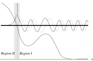
In one dimension, it is easy to distinguish two types of regions in configura- tion space (see fig.1.1): the ‘classically allowed region’ I (where E > V(x)) is accessible for a classical particle, while the region II (E < V(x)) is classically forbidden.

x Region I

Region II

Figure 1.1: Classically allowed (I) and forbidden (II) regions for a particle of energy E in a potential V(x). The thin solid and dotted lines show real and imaginary parts of the WKB wave function (1.11). The waves are not correctly matched at the transition point.

Consider in more detail the region I in fig.1.1. The momentum (1.8) is real there, and the WKB wave function (1.11) is the natural generalisation of a plane waveexp (±ipx/¯h)that would propagate towards the right (left) if the momen- tum p were spatially constant (we conventionally use the factor exp(−iEt/¯h) for the time-dependence of the wave function). The wave function (1.11) being complex, we show its real and imaginary parts. They are oscillating and behave as cosφ(x) and sinφ(x)(sinusoidal curves with a phase difference π/2). From the relative positions of the maxima in the real and imaginary part, we deduce that the phase φ(x) increases towards the right, the figure thus shows a wave propagating to the right. In agreement withDEBROGLIE’s formulaλ= ¯h/p, the phase varies slowly (the wave length is large) when the classical momentum p(x)is small (above the barrier in the figure), while it varies rapidly whenp(x) is larger.

As regards the envelope of the oscillations, it follows an opposite trend: the magnitude of the wave function |ψ(x)| = C/^qp(x) is larger when the particle moves more slowly. This is because the quantity|ψ(x)|²dx = ρ(x)dx gives the probability to find the particle in the intervalx . . . x+ dx. Since for a stationary flow in one dimension, the equation of continuity gives∂j/∂x = −∂ρ/∂t = 0, the particle current density j(x) = ρ(x)p(x)/m is conserved. This gives j(x) = const., and we have

|ψ(x)|² =ρ(x) = mj

p(x). (1.12)

Physically speaking, the probabilityρ(x)dx=jdt is proportional to the timedt the particle needs to move across the interval x . . . x+ dx at the local velocity p(x)/m. Note that we cannot predict at which particular time the particle will cross the position x because the flow (the wave function) is stationary by as- sumption. We do not know the time when the particle started, and therefore, only a probabilistic prediction may be given.

Finally, we note from (1.12) that the WKB wave function diverges at a ‘clas- sical turning point’ where the velocity vanishes. This divergence is clearly visi- ble in figs.1.1, but it isunphysical(it is not reproduced by the exact solution of the SCHRODINGER¨ equation).

Forbidden region

Turn now to region II in fig.1.1 that is classically forbidden because the potential is larger than the energy. The momentum

p(x) = ^q2m(E−V(x)) = i^q2m(V(x)−E)

is then purely imaginary, and the wave function (1.11) shows a sort of expo- nential growth or decay. The local decay constant is approximately equal to

±|p(x)|. The wave function shown in the figure decreases exponentially when the position x moves into the forbidden region. Whether this is physically ac- ceptable depends on the overall behaviour of the potential.

Tunnelling through a barrier

The situation shown in fig.1.1 would be false if there were an additional po- tential well to the left, as shown in fig.1.2. Indeed, in this case, the particle is predominantly localised in the potential well, and (at least if the barrier is quite thick) the wave function must decrease when the positionxmoves towards the right into the forbidden region. On the other hand, once the barrier has been crossed, the waves ‘leaks’ out of the exponentially small tail towards the right.

A wave propagating to the right in region I is therefore physically reasonable.

This process is the ‘tunnel effect’, and we shall derive a simple formula for the tunnelling rate below.

Reflection from a barrier

Figure 1.3 shows the case that the forbidden region II extends up tox =−∞.

The exponential decay towards the left (or increase towards the right) is

Region I x Region II

Region III

Figure 1.2: Wave function leaking out of a potential well (region III) through a barrier (II) into an allowed region (I). The waves are not matched at the transition points. The wave in region I is not drawn to scale.

x Region I

Region II

Figure 1.3: Reflection from a potential barrier. The waves are not correctly matched across the turning point, and the incident wave is missing in region I.

then physically reasonable because otherwise the total probability of being in the forbidden region would be infinite. But now, the wave function in re- gion I is not correct: classically, one would expect that there is also a flow of particles incident from the right and being reflected from the potential bar- rier. The wave function must therefore contain also a term proportional to exp (−i^Rxp(x⁰)dx⁰/¯h), describing a wave moving towards the left. We discuss below how in this case of barrier reflection the WKB solutions are matched across the turning point.

Open questions

The discussion presented so far leads us naturally to a number of questions.

They are going to be analyzed in the following sections of this chapter.

• What is a precise criterion for the validity of the WKB approximation?

• How are the WKB wave functions to be matched across the boundary between the classically allowed and forbidden regions? We anticipate that this matching depends on the global behaviour of the potential for the chosen energy (particle trapped in a well or incident from infinity, e.g.).

• The WKB wave functions should also be able to yield approximations for, e.g., the quantised energy levels in a potential well or the tunnelling rate through a barrier. We would also like to know in what regime these ap- proximations are valid.

• How is it possible to remove the divergence ∝1/^qp(x)of the WKB wave functions at a turning point without losing precision far away from the turning point?

• How may the above treatment be generalized to multi-component (‘spinor’) wave functions that are no longer scalar complex functions?

And what about spatial dimensions larger than one?

1.2 Validity criteria

Naive estimate

The quantum mechanics textbooks often quote the following condition of valid- ity of the WKB approximation: in the SCHRODINGER¨ equation (??), we neglect

the term containing¯hcompared to the others. This is reasonable if

¯ h 2m

d²S dx²

1 2m

dS dx

!2

(1.13a) where the right hand side is a particular term representing the ‘large’ terms in (??). This condition may be written in terms of the local classical momentum p(x)or, equivalently, the local wavelengthλ(x) = ¯h/p(x), and we get

¯ hdp

dx

p²(x) or

d dx

¯ h p(x)

=

dλ(x) dx

1. (1.13b)

The WKB approximation is thus valid whenthe local wavelength changes slowly.

As a rule of thumb, the gradient d/dx in (1.13b) is of the order of 1/a where a is a classical length scale (that may depend on position and energy). We thus recover the intuitive idea that the DE BROGLIEwave length must be small compared to the classical length scales of the problem.

It is a simple exercise to re-write the validity condition (1.13b) in terms of the classical force acting on the particle:

¯hm|F(x)| p³(x) (1.13c) Note that both conditions (1.13b, 1.13c) predict a breakdown of the WKB ap- proximation at classical turning points because of the vanishing momentum p(x).

On the other hand, if the wave length is spatially constant, the WKB approx- imation is valid (it is even exact).

More careful estimate

Recall that the WKB approximation is based on the expansion (1.6) of the action function. This expansion is accurate if higher-order terms become successively smaller in the limit of small¯h. We thus obtain the condition

. . .¯h²|S₂| ¯h|S₁| |S₀| (1.14) where we have also included the second order term S₂. This term may be explicitly calculated from the SCHRODINGER¨ equation, with the result (primes denotes differentiation with respect toxand S is now a complex quantity that also contains the amplitude calledAbefore):

dS₂ dx = 1

2S₀⁰

iS₁⁰⁰−(S₁⁰)² (1.15)

This expression allows to calculate condition (1.14) for a given problem. One has to be careful with the arbitrary constants that appear in the Sn. In prac- tice, it seems a good choice to fix a reference point x_r and to evaluate condi- tion (1.14) for the differences¯hⁿ⁻¹[S_n(x)−S_n(x_r)].

There is anadditional conditionthat is due to the fact that the action appears in the exponent of the wave function. We have to impose that the termhS¯ ₂ is small compared to unityto assure that we make only a small error in the wave function:

¯h|S₂| 1 (1.16)

If this is case, we may expand exp

i

¯ h

S₀+ ¯hS₁+ ¯h²S₂

≈ψ_WKB(x) [1 + i¯hS₂(x)]

and get a correction that is small relative to the WKB wave function. IfhS¯ ₂ = 0.01, say, then the WKB wave function is accurate to one percent. Of course, condition (1.16) has also to be calculated explicitly for a given problem.

Spatially constant wave length. This an example where it is easy to obtain the actionsS_n explicitly. The momentumpis constant, and choosingx_r = 0as reference point, we get

S₀(x) = px (1.17)

S₁(x)−S₁(0) = i

2logp(x)

p(0) = 0 (1.18)

S2(x)−S2(0) = 0 (1.19)

Both inequalities in condition (1.14) are therefore fulfilled. Furthermore, since S₂ is constant, one is free to chooseS₂ = 0, and thus satisfy condition (1.16).

More examples are given in problem ??. We finally note that a good check for the WKB approximation is the comparison with exactly solvable potentials.

This will also be done both in the lecture and in the problems.

1.3 Matching rule at a turning point

Langer has found the following ‘connection formula’ for the WKB waves at a single turning point:

2C

qp(x)sin

π 4 + 1

¯ h

Z x0

x

p(x⁰)dx⁰

←−

allowed region (I)x < x0

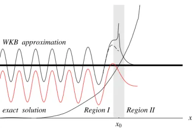
x⁰ x Region I Region II

WKB approximation

exact solution

Figure 1.4: WKB wavefunction that is correctly matched at a turning point x0. The red curve gives the (numerically computed) exact solution to the Schr¨odinger equation. It is shifted down because otherwise it would be in- distinguishable from the WKB solution almost everywhere. The dashed curve continues the sine function in (1.20) without the1/^qp(x)divergence.

←− C

q|p(x)|exp

−1

¯ h

Z x x0

|p(x⁰)|dx⁰

(1.20) forbidden region (II)x > x₀

The arrow indicates that we got this formula by imposing a boundary condition in the forbidden region (the wave function must decrease).

The WKB wave function that results from the connection formula (1.20) is plotted in fig.1.4 and compared to the exact solution of the SCHR¨ODINGER

equation that was computed numerically.

Comments

• If the allowed region is located to the right of the turning point (the po- tential has a negative slope), the connection formula becomes

C

q|p(x)|exp

−1

¯ h

Z x0

x

|p(x⁰)|dx⁰

−→

forbidden region (II)x < x0

−→ 2C

qp(x)sin

π 4 + 1

¯ h

Z x x0

p(x⁰)dx⁰

(1.21) allowed region (I)x > x0

Short cut: simply write the integral in such a form that their values in- crease whenxmoves away from the turning point.

• We observe in fig.1.4 that the sinusoidal oscillations in the allowed region are positioned in such a way that the inflexion point of the sine occurs at the turning point x = x₀ (although the amplitude of the WKB wave function still diverges). This is shown by the dashed curve in fig.1.4 where the sine function is plotted without the diverging prefactorp(x)^−1/2.

• There is a phase jump of π +π/2 ≡ −π/2between the incident and re- flected wave. It is interesting that this phase jump is intermediate be- tween the reflection at a ‘fixed’ end (phase shift π) and at a ‘loose’ end (zero phase shift) of a string.

• The reflection probability is unity. More precisely, the reflection coefficient R is defined by the following form of the wave function in the allowed region:

ψ(x) =C[ψ_inc(x) +R ψ_refl(x)] (1.22) If we choose incident and reflected waves in the WKB form (1.11),

ψ_inc,refl(x) = 1

qp(x) exp

±i

¯ h

Z x x0

p(x⁰)dx⁰

we get from (1.20) a reflection coefficient R =−i

and hence a reflection probability |R|² = 1. On the other hand, there is zero transmission into the forbidden region. Both properties are related to the fact that the wave function is real over the entire x-axis. (Argue that this is a consequence of current conservation.)

• The connection formula (1.20) isunidirectionalin the sense that we have started from an asymptotic condition in the forbidden region (exponential decay of the wave function). The other direction of the connection for- mulas is needed when a tunnelling problem is studied: one then imposes that in the allowed region, there is only an outgoing and no incoming wave. This case gives rise to both exponentially decaying and increasing solutions in the forbidden region. We study it in more detail in the follow- ing subsection. There has been a long discussion about the directionality of the connection formula; see Berry & Mount (1972) for a review of this point.

• We can derive a criterion for the validity of the above approach. Start with linearising the potential in an interval x0−a . . . x0+awhose length 2a must be at least a few w = (¯h²/2mF)^1/3. This characteristic length emerges from dimensional analysis of the Schr¨odinger equation in the linear potential: it gives the physical scale of the exact solutions which are provided by AIRY functions. The condition a w is needed because otherwise we cannot use the asymptotic expansions of the AIRY function towards the ends of the interval. This means¹

a³ w³ = ¯h²

2mF (1.23)

This condition is of course valid if ‘¯h is sufficiently small’. On the other hand, it becomes violated if the classical length scale a gets too small.

This length may be, for example, the distance to another turning point. If this second point comes closer than a few w’s, it is in general no longer possible to treat them separately. In this case, one has to solve exactly a problem with two turning points and match the solution to the WKB wave functions that are valid at a larger distance.

1.4 Bohr-Sommerfeld quantisation

As an important application of LANGER’s connection formula, we discuss here the quantum-mechanical tunnelling through a potential barrier and the semi- classical quantisation rule in an isolated potential well.

1.4.1 WKB quantisation rules

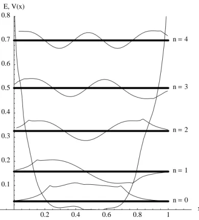
The quantisation of energy in a potential well is a second important application of LANGER’s connection formula. In fig.1.5, the results that may be obtained for a generic potential are sketched. We suppose that the ‘walls’ of the well are impenetrable and neglect tunnelling. The physically acceptable wave function must therefore decay exponentially in the forbidden regions x < x₁, x > x₂ (where x_1,2 denote again the turning points). If the turning points are suffi- ciently far apart, we may use the connection formula twice to find the wave function in the allowed regionx₁ < x < x₂. The key point is that for a generic

1It is interesting that we can get (1.23) from the previously derived condition (1.13b) by estimatingp'¯h/a. This is the momentum of a particle in the ground state of a box with length a.

0.2 0.4 0.6 0.8 1 x 0.1

0.2 0.3 0.4 0.5 0.6 0.7 0.8

E, V(x)

n=0 n=1 n=2 n=3 n=4

Figure 1.5: Potential well with quantised states, obtained with the semiclassical approximation.

choice of energy, we get two expressions for the wave function that do not match. To be explicit, we get from (1.21) the wave function forx > x₁:

ψ1(x) = C

qp(x)sin

π 4 + 1

¯ h

Z x x1

p(x⁰)dx⁰

, (1.24)

while the connection formula (1.20) at the turning pointx₂ gives ψ₂(x) = C⁰

qp(x) sin

π 4 + 1

¯ h

Z x2

x

p(x⁰)dx⁰

. (1.25)

To compare these two functions, we write

Z x2

x

p(x⁰)dx⁰ =

Z x2

x1

p(x⁰)dx⁰ −

Z x x1

p(x⁰)dx⁰

= S(x1, x2)−

Z x x1

p(x⁰)dx⁰

where S(x1, x2) is the classical action integral for half an oscillation period in the well:

S(x₁, x₂) =

Z x2

x1

q

2m(E−V(x)) dx. (1.26)

We thus get

ψ₂(x) = C⁰

qp(x)

sin S(x₁, x₂)

¯

h +π 2 −π

4 − 1

¯ h

Z x x1

p(x⁰)dx⁰

!

This function is identical to (1.24) when the first two terms in the argument of the sine are an integer multiple ofπ. We may then choose the constantC⁰ equal toCup to a sign. This is the WKB quantisation rule: the classical action must be a half-integer multiple of the Planck constant:²

S(x₁, x₂) = n+ ¹₂π¯h, n = 0, 1, 2, . . . (1.27) C⁰ = (−1)ⁿC,

Observe that depending on the parity of the quantum number, the eigenfunc- tions decay with the same sign or with different signs in the forbidden regions (see fig.1.5). This is reminiscent of the well-defined parity of the eigenfunctions in an even potential well.

The accuracy of the semiclassical approximation can be checked from the validity criteria given before: one has to compare the distance between the turning points to the length scalesw_1,2 that appear in the WKB matching pro- cedure at the turning points. The ground state wave functionn = 0shown in fig.1.5, e.g., is certainly inaccurate because it shows inflexion points in a region where both the potential and the wave function do not vanish.

It is not too easy to determine eigenvalues numerically, and for this reason the semiclassical formula (1.27) is useful, too. Typically one uses the ‘shoot- ing method’: first, a trial value for E close to the semiclassical eigenvalue is chosen; then the Schr¨odinger equation is solved starting from a point deep in the forbidden region x < x₁. This solution typically diverges exponentially in the forbidden regionx > x₂. Then the energy is changed until the sign of this divergence changes. One can then use successive bisections to find the energy where the wave function becomes smaller than a preset accuracy. It also helps to study the semiclassical wave functions when choosing the initial and final points in the forbidden regions.

Examples

For aharmonicpotential, the WKB quantisation procedure reproduces the exact eigenvalues. Although this happens by accident (check it from the WKB validity

2The integernmust be non-negative because the action integral (1.26) is positive.

criteria), it is nevertheless a simple nontrivial example. The action integral is

√2m

Z x2

x1

qE− ^m₂ω²x²dx=mωπx²₂

2 = πE ω and the quantisation rule (1.27) givesE =E_n=n+ ¹₂hω.¯

For alinearpotential well that is closed by an infinite potential barrier (Wal- lis & al., 1992), the WKB quantisation rule applies with a slight modification:

there is no phase jumpπ/4at the infinite barrier. We thus get

√2m

Z x2

0

√E−F xdx=√

2mF2(E/F)^3/2 3

=! n+¹₄π¯h

=⇒ E_n=

3π 2

n+¹₄

2/3

F w (1.28)

wherewis the length scale for the linear potential introduced in (??). Note the different power lawE ∝n^2/3 as compared to the harmonic potential.

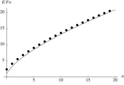
Since we know the exact wave function for the linear potential, we can evaluate the accuracy of the WKB approximation. The exact wave function is given by a displaced AIRY functionAi((x−x2)/w), wherex2 =E/F is the right turning point. The boundary condition at x₁ = 0 imposes the quantisation of energy:

Ai(−E/F w) = 0

The energy eigenvalues are thus proportional to the zeros of the AIRYfunction, with the quantity F w giving the energy scale. Figure 1.6 compares this result with the semiclassical prediction. One sees that for n ≥ 10 the agreement is already quite good.

Other examples are the Eckart or Morse wells V(x) = V0

cosh²(κx), V(x) = V₀e^−κx−1²

where exact eigenfunctions and eigenvalues may be obtained. These potentials are studied as problems.

1.4.2 Barrier tunnelling

(Material not covered in WS 2012/13.)

Consider a wave that is scattered by a potential barrier, as shown in fig.1.7. We shall suppose that the particle is incident fromx → −∞where the potential is small,

5 10 15 20 n 5

10 15 20

E/Fw

Figure 1.6: Quantised energy values in a linear potential well. Dots: exact zeroes of the AIRY function; line: semiclassical prediction (1.28).

and that its energy is below the barrier top. We have two turning pointsx1,2 and the following asymptotic behaviours:

x→ −∞: ψ(x) =incident wave+Rreflected wave x→+∞: ψ(x) =Ttransmitted wave

Note that to the right of the barrier, there is only a single transmitted and no incident wave. As a consequence, the wave function will be complex. We shall construct a suitable superposition of real wave functions, and for this purpose, we need a second wave function that solves the turning point problem.

Matching with an exponentially growing wave at a turning point. In the previous section, we constructed a physically acceptable wave function at a reflecting

x₂ E

x₁

Figure 1.7: Reflection and transmission of a wave from a potential barrier.

turning point. We consider here the opposite case, namely a wave function that di- verges in the forbidden region. This divergence is not a real problem because for the barrier shown in fig.1.7, the forbidden region has a finite extension.

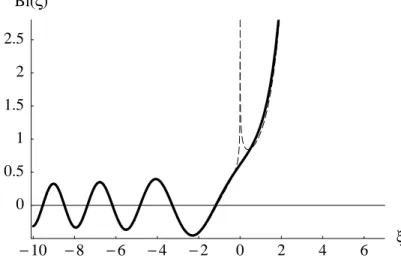
The calculation is quite parallel to the one in the previous section. We choose again the dimensionless variable ξ with ξ > 0being the forbidden region. The AIRY equa- tion (??) has the second solutionBi(ξ)that is sketched in fig.1.8. It shows an exponen-

−10 −8 −6 −4 −2 0 2 4 6 ξ 0

0.5 1 1.5 2 2.5

Bi(ξ)

Figure 1.8: The AIRY function Bi(x) (solid curve) and its asymptotic forms (dashed curves).

tial growth in the forbidden region. The asymptotic behaviours are (see problem??)

ξ −1 : Bi(ξ) ≈ 1

√π(−ξ)^1/4cos 2

3(−ξ)^3/2+π 4

(1.29a) ξ1 : Bi(ξ) ≈ 1

√πξ^1/4 exp 2

3ξ^3/2

(1.29b) Note the factor of 2 that is missing in (1.29b) and the cos instead of the sin in (1.29a).

When we compare these formula to the WKB wave functions in the vicinity of the turning point, we arrive at the following connection formula

D pp(x)cos

π 4 + 1

¯ h

Z x0

x

p(x⁰)dx⁰

−→

allowed region (I)x < x0

−→ D

p|p(x)|exp 1

¯ h

Z x x0

|p(x⁰)|dx⁰

(1.30)

forbidden region (II)x > x0

Berry & Mount (1972) quote the warning of Fr¨oman & Fr¨oman (1965) that this connec- tion formula has to be taken with much care. Indeed, eq.(1.30) may only be understood

as a relation between the asymptotic behaviour of this (unphysical) wave function. In numerical work, it is impossible to be sure that the decaying exponential has a nonzero coefficient – this does not change the numerical results just because the coefficient is multiplied by a small number. But a nonzero coefficient inevitably gives an admixture of a sine function in the allowed region and changes the phase of the standing wave.

The derivation used here shows that (1.30) simply gives the asymptotic form of the other linearly independent solution to the SCHR¨ODINGERequation.

The turning point x₂. The status of the connection formula (1.30) thus clarified, we can write it down for the turning point x₂ in fig.1.7. In this case, the forbidden region is located to the left ofx2, and the connection formula becomes

D p|p(x)|exp

1

¯ h

Z x0

x

|p(x⁰)|dx⁰

←−

forbidden region (II)x < x₀

←− D pp(x)cos

π 4 + 1

¯ h

Z x x0

p(x⁰)dx⁰

(1.31)

allowed region (I)x > x₀ If we want to get a transmitted wave propagating to the right

x > x2 : ψ(x) = N pp(x)exp

i

¯ h

Z x x2

p(x⁰)dx⁰+iπ 4

,

we thus have to superpose the wave functions (1.21, 1.31) with the coefficients 2C = iN, D=N

whereN is a global normalisation constant. ‘Under the potential barrier’ (in the for- bidden region), the wave function is a superposition of exponentially growing and decreasing waves with weights given byC, D. We now match this superposition to incident and reflected waves at the first turning pointx₁. To simplify the comparison, we write

Z x2

x

|p(x⁰)|dx⁰ = Z x2

x1

|p(x⁰)|dx⁰− Z x

x1

|p(x⁰)|dx⁰

= ¯hW − Z x

x1

|p(x⁰)|dx⁰

where W is a positive number that depends on the energy and the behaviour of the potential in the forbidden region

W =

√2m

¯ h

Z x2

x1

q

V(x⁰)−Edx⁰ (1.32)

The turning pointx₁. The wave function that arrives from the right at the turning pointx₁is thus of the form

x > x₁ : ψ(x) = N p|p(x)|

e^Wexp

−1

¯ h

Z x x1

|p(x⁰)|dx⁰

+ + i

2e^−Wexp 1

¯ h

Z x x1

|p(x⁰)|dx⁰

(1.33) The first term decreases whenxmoves into the forbidden region and therefore connects to the regular solution of formula (1.20). For the second, increasing term we need again the connection formula (1.30) for the ‘unphysical’ solution. We finally get, in the allowed regionx < x₁, the following superposition of incident and reflected waves

x < x₁ : ψ(x) = N pp(x)

α_incexp i

¯ h

Z x x1

p(x⁰)dx⁰

+ +α_reflexp

−i

¯ h

Z x x1

p(x⁰)dx⁰

where the coefficients are given by

α_inc = e^W+iπ/41 +¹₄e^−2W, (1.34)

α_refl = e^W−iπ/41−¹₄e^−2W. (1.35) Using the fact that the WKB wave functions have unit flux, we thus get the following reflection and transmission coefficients:

R = −i1−¹₄e^−2W

1 +¹₄e^−2W, |R|²≈1−e^−2W (1.36a) T = e^−W

1 +¹₄e^−2W, |T|²≈e^−2W (1.36b) where the approximations are valid whenW 1(semiclassical regime: ‘action inte- gral’ (1.32) large compared to ¯h). We observe that in this regime, the transmission through the barrier is extremely small: the current is transported to the second turning pointx₂ only via the ‘tail’ of the exponentially decaying wave that enters the forbidden region atx1.

Comments. One may verify from (1.36) that current conservation,|R|²+|T|² = 1, is also valid ifW is not large. In this limit, however, the turning pointsx1,2 approach each other too closely to allow for a separate application of the single turning point connection formula, and the results (1.36) cease to be valid. In problem??, you are invited to derive an approximation that covers this regime. One result of this approxi- mation is that when the incident energy coincides with the barrier top, both reflection and transmission probabilities|R|²and|T|² are equal to ¹₂. For energies below the bar- rier, the transmission decreases rapidly to exponentially small values. But even when

the energy is larger than the barrier top, there is a nonzero probability of reflection. It becomes very small, too, when the energy is much larger than the barrier top.

We can get a simple estimate for the width in energy of the transition zone where the transmission goes over from close to zero to close to unity. Close to the barrier top, we approximate the potential by an inverted parabola with second derivative V⁰⁰ =

−mω². For an energy ∆E below the barrier top, two turning points exists and are spaced

a= s

8∆E mω²

apart. In the estimate (1.23) for the validity of the single turning point connection formula, we have to require a w where w depends on the potential slope at the turning points. Using the definition (??) of the width w, we find that our result is valid provided∆E ¯hω/8, i.e., the energy is sufficiently below the barrier top. This condition implies in turn that the transmission through the barrier is very small since we have (using again a parabolic shape for the barrier top)W ≈ π∆E/¯hω π/8 ≈ 0.393.

Remark. LANGER was not the first to use the patching procedure with the AIRY function at a turning point. This method was already employed by JEFFREYS (1923) and KRAMERS(1926). The other two people in what is sometimes called the JWKB approximation are WENZELand BRILLOUIN.

1.5 Uniform asymptotic approximations

1.5.1 The basic idea

LANGER’s connection formula tells us how to glue the WKB wave functions together on both sides of a turning point. But we still have a wave function that is made up of two or three different expressions, depending on whether the AIRY function is used close to the turning point or not. It would be great if we had a single formula that is valid throughout the transition region. Such a kind of formula exists, and in fact LANGERalready wrote it in his papers.

Langer (1937) was able to derive auniform asymptoticapproximation to the wave function at a single turning point. His results were subsequently gener- alised, and are based on the following idea (Berry & Mount, 1972). We want an approximate solution of the Schr¨odinger equation³

− d²ψ

dx² +W(x)ψ = 0, (1.37a)

3To simplify the notation, we write the potential in the formW(x) = (2m/¯h²) [V(x)−E].

and we know the exact solutionφ(y)to a ‘similar’, but simpler potentialU(y),

− d²φ

dy² +U(y)φ= 0. (1.37b)

This equation is called the ‘comparison equation’. We conjecture that the wave functionφ(y)will be similar toψ(x)and may be obtained by ‘streching or con- tracting it a little and changing the amplitude a little’ (Berry & Mount, 1972, p.343). We thus make theansatz

ψ(x) = f(x)φ(y(x)) (1.38)

where f(x) and y(x) are functions to be determined. Insert this into the SCHR¨ODINGERequation (1.37a) and find, using (1.37b):

− d²f

dx²φ− dφ dy 2df

dx dy

dx +fd²y dx²

!

−f dy dx

!2

U φ+f W φ= 0. (1.39) We can get rid of the first derivativedφ/dyby choosing

f = dy dx

!−1/2

(1.40) Then we may divide by f φand find an equation for the ‘coordinate mapping’

y(x):

− dy dx

!1/2

d² dx²

dy dx

!−1/2

− dy dx

!2

U(y(x)) +W(x) = 0 (1.41) We now make an approximation that is motivated by our idea that the co- ordinatesxand ydiffer only by small strechtings. We can then expect that the second derivative in (1.41) to be ‘small’, and may neglect it.⁴ We then get the first-order differential equation

dy

dx =± W(x) U(y(x))

!1/2

(1.42) With the initial conditiony(x₀) = y₀, we find the following implicit solution

Z x x0

q

W(x⁰) dx⁰ = ±

Z y y0

q

U(y⁰) dy⁰ (1.43a)

Z x0

x

q−W(x⁰) dx⁰ = ±

Z y0

y

q−U(y⁰) dy⁰ (1.43b)

4This procedure is similar to what we did at the start to get the WKB approximation.

where the choice depends on the sign ofW(x), i.e., whetherxis in an allowed (W(x)<0) or forbidden (W(x)>0) region (see footnote 3 on p. 23).

Once we have computed y(x) by inverting these equations, we have the following approximation for the wave function

ψ(x)≈

"

U(y(x)) W(x)

#1/4

φ(y(x)) (1.44)

We shall see that this solution is valid for the whole range of x, even close to turning points.

This method works only when the coordinate mappingx7→y(x)is bijective, i.e., when the derivativedy/dxis nowhere zero nor infinite. Looking at (1.42), we observe that this implies that the zeros of the potentials W(x) and U(y) are mapped onto each other. In particular, both potentials must have the same number of turning points. ‘We thus have what is potentially a very powerful principle: in the semiclassical limit all problems are equivalent which have the sameclassical turning-point structure’ (Berry & Mount, 1972, p.344).

1.5.2 Examples

Recover the standard WKB waves. The first example is a classically allowed region without turning points. The function W(x) = −p²(x)/¯h² then vanishes nowhere, and we may takeU(y)≡ −1. The comparison equation reads

d²φ

dy² +φ = 0

and its solutions are plane waves φ = exp(±iy). The coordinate mapping is obtained from the solution of

dy

dx =±p(x)

¯

h . (1.45)

The amplitude function (1.40) is thus equal tof(x) = (¯h/p(x))^1/2, and we get the propagating WKB waves

ψ(x)≈ C

qp(x) exp

±i

¯ h

Z x x0

p(x⁰) dx⁰

.

These expressions are no longer valid at turning points because the mapping x 7→ y then becomes singular [see (1.45)]. Similarly, we can derive the WKB solutions in classically forbidden regions by choosingU(y)≡1.

A single turning point. If the potentialW(x) =−p²(x)/¯h² has a simple turn- ing point at, say,x0, we are advised to take a comparison potential with a simple zero, say,U(y) =y. This gives the AIRYequation

−d²φ

dy² +yφ= 0

with the general solution φ(y) = αAi(y) +βBi(y). To compute the coordinate mapping, we observe from (1.42) that the classically allowed regionW(x) <0 must be mapped ontoy <0, and vice versa. This fixes the sign of the derivative dy/dx. Suppose for definiteness that the allowed region isx < x₀. We thus get from the implicit coordinate mapping (1.43)

2

3(−y)^3/2 = 1

¯ h

Z x0

x

p(x⁰) dx⁰, x∈allowed, y <0 (1.46a) 2

3y^3/2 = 1

¯ h

Z x0

x

|p(x⁰)|dx⁰, x∈forbidden, y >0 (1.46b) If the allowed and forbidden regions are located the other way round, one simply has to change the order of the integration limits. The mapping (1.46) thus makes those pointsx,y correspond for which the classical action integral (divided by ¯h) has the same value. Recalling the expansion of the action in the vicinity of the turning point, we also conclude that the mapping x 7→ y = (signV⁰(x₀))(x−x₀)/w is approximately linear there. This justifiesa posteriori the neglect of the second derivative in (1.41) around the turning point (the functiondy/dxis approximately constant).

Finally, we get the following uniform approximation for the wave function for a potential with a single turning point:

ψ(x) =C y(x) p²(x)

!1/4

αAi(y(x)) +βBi(y(x)) (1.47) It is a simple exercise to check that far from the turning point, this expression goes over into both connection formulas (1.20, 1.30): the argument y(x) is then large in magnitude, and we may use the asymptotic expansions of the AIRY functions. Because of the form (1.46) of the coordinate mapping, we then recover exponentials or trigonometric functions whose arguments are classical action integrals.

Explicit example: uniform expansion for the BESSEL functions. To illus- trate the power of the uniform expansion, we shall derive a uniform expansion

of the BESSELfunctions. It has been shown in problem??that the BESSELfunc- tion Jn(kr) is the physically acceptable solution to the radial SCHR¨ODINGER

equation

− d²

dr²J_n− 1 r

d

drJ_n+ n²

r²J_n=k²J_n

where r is the radius in (two-dimensional) polar coordinates. To simplify the following calculations, we measurer in units of1/k and putk = 1. We get rid of the first derivative in the BESSELequation by putting

J_n(r) = 1

√rj(r)

The physical boundary condition at the origin is now thatj(r)is of orderr^n+1/2 there. The centrifugal potential then changes to

n²

r² 7→ n²− ³₄ r² ≡ L²

r², and we find the following potential

W(r) = L² r² −1

This potential has a single turning point at r₀ = L (note that this zero does not exist when n = 0, we exclude this case). We map the forbidden region 0< r < r₀ onto the half-axisy >0of the AIRY equation using (1.46) and get

2

3y^3/2 =

Z r0

r

q

W(r⁰) dr⁰ =

Z r0

r

q

L²−r⁰²dr⁰ r⁰

= Llog L+√

L²−r² r

!

−√

L²−r²

Similarly, the allowed regionr₀ < r <∞is mapped ontoy <0using 2

3(−y)^3/2 =

Z r r0

q

r⁰²−L²dr⁰ r⁰

= LarcsinL r +√

r²−L²−Lπ 2.

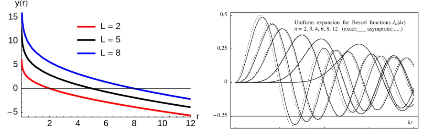
The prefactor of the wave function is given by(y(x)/W(x))^1/4.The coordinate mapping is illustrated in Fig.1.9(left) for different values of L. Note how y(r) is smooth atr=L=r0.

Using the boundary condition that the BESSELfunctionsJ_n(kr)vanish at the origin (forn ≥1), we finally get the following asymptotic expression

J_n(kr) = C y(kr) n²−³₄ −k²r²

!1/4

Ai(y(kr)) (1.48)

The uniform approximation cannot determine the global prefactorC. but com- paring with the standard asymptotic form of the BESSEL functions for large argumentkr n, we findC = √

2. Comparing to the standard asymptotics, one also finds that the uniform expansion is valid if the effective angular mo- mentumLis large compared to unity.

In fig.1.9(right), we compare the uniform expansion (1.48) to the exact BESSELfunctionsJ_n(kr)for several values ofn. We observe that the agreement

2 4 6 8 10 12r

-5 0 5 10 15

yHrL

L=2 L=5 L=8

20

−0.25 0 0.25 0.5

Uniform expansion for Bessel functions J_n( )kr n=2, 3, 4, 6, 8, 12 (exact:___ asymptotic:...)

kr

Figure 1.9: Uniform asymptotic expansion (1.48) for the BESSELfunctions.

is quite good over the entire range of the argumentkrand becomes much better when the ordern(and hence the effective angular momentum L) increases.

1.6 Multi-state dynamics

Motivation

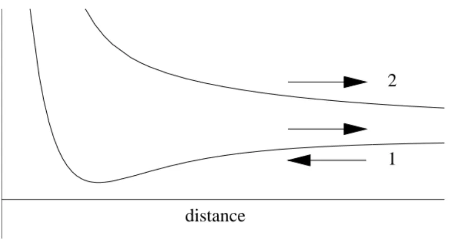
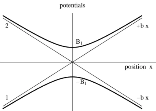
There are a number of fields in physics where a particle or a particle system may exist in different states. These states are, typically, subject to different potentials. An example is a molecule made of two atoms. Depending on the electronic state of the atoms, the relative motion is governed by attractive or repulsive potentials (see figure 1.11). How does the Schr¨odinger equation look like for such a system? It still depends on a single coordinate (the relative distance of the two atoms in the above example), but we have to use a wave function with two components, each one giving the probability amplitude to be in the stateα = 1, 2. We shall call such an objectΨ(x)a ‘spinor’. Similarly, the potential becomes a2×2matrix.

1.6.1 Light polarization and geometrical optics

Another example with a similar formal structure is electrodynamics in the limit where the wavelength is small, also known as geometrical optics. We know that the electromagnetic field is a vector field, described by the Maxwell equations

∇ ×B+ iω

c²ε(x)E = 0

∇ ×E−iωε(x)B = 0 (1.49)

This is written in SI units, at a fixed frequencyωand in a medium with permit- tivity ε(r, ω) (also known as dielectric function). We assume in the following that ε = n² is real. The symmetry between E and B can be restored by re- scaling the magnetic field tocB =H. We introduce the wavenumberk =ω/c.

We consider the asmptotic limit of a small wavelength whereλ = 1/k → 0 plays the role of the Planck constant. This motivates theAnsatz

E(x) = E(x) e^ikS(x), H(x) = H(x) e^ikS(x) (1.50) with slowly varying vector amplitudes E and H. The function S(x) is called theeikonal. Putting this into the Maxwell equations (1.49), we find to leading order inλ:

∇S× H+n²E = 0, ∇S× E − H= 0 ⇒ (∇S)² =n² (1.51) which is known as the eikonal equation. Note the similarity to the WKB result for the action. We can make the formal analogy n²(x) ↔ E −V(x) to the potential of classical mechanics. In the vector case we are dealing with here, we get additional information: the amplitude vectorsE andHare both orthogonal to the gradient ∇S, the three forming a so-called Dreibein. This is sometimes called an ‘solvability condition’: it corresponds to constraints that are built into the partial differential equations, and that the solutions must satisfy (similar to

∇ ·B = 0).

To solve the eikonal equation, one introduces thelight rays r(s)as the field lines of the vector field∇S. By definition of field lines, they solve the differen- tial equation

dr

ds ∼ ∇S[r(s)], dr

ds = ∇S[r(s)]

n[r(s)] (1.52)

where in the second step, we have chosen the parametersto be the arc length of the ray: recall that the vector∇S/n is a unit vector according to the eikonal equation (1.51). Eq.(1.52) is still not very useful because it involves the func- tion∇S that we do not know yet. One can eliminate the eikonal, however, by

calculating the ‘acceleration’ (second derivative) of the ray d

dsn[r(s)]dr

ds =∇n[r(s)] (1.53) This is the basic equation of geometrical optics. Note again the analogy to mechanics, with∇nplaying the role of the ‘force’. In a homogeneous medium, the rays are therefore straight lines.

Intensity and polarization transport. Along a light ray (more precisely: a bundle of rays), one can show that the electromagnetic energy density is flow- ing with a current density given by the Poynting vector. By analogy to the continuity equation,

∇ ·ReE^∗×H= 0 (1.54)

(a factorn may be missing here). For the transport of the polarization vectors, we introduce the (complex) unit vectors

e= E

|E|, h= H

|H| (1.55)

and find (see the book by Born & Wolf (1959) for details) n(r)de

ds =−(e· ∇logn)∇S (1.56)

To interpret this equation, consider the simple case that the ray is lying in a plane spanned by the vectors∇S (the tangent or velocity vector) and∇n (the acceleration). Ife is perpendicular to this plane, then from Eq.(1.56), it does not change and remains perpendicular. On the other hand, if e is in the ray plane, Eq.(1.56) forces it to change. Using the fact thate and∇S are perpen- dicular [solvability condition (1.51)], we can re-write Eq.(1.56) into

n(r)de

ds = −(e· ∇logn)∇S+ (e· ∇S)

| {z }

= 0

∇logn

= (∇S× ∇logn)×e (1.57)

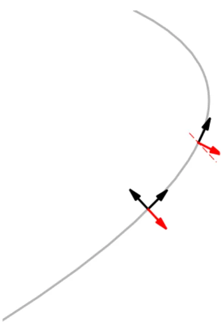
This means that the polarization vector is rotating in the ray plane (around an axis∇S× ∇lognperpendicular to the ray plane). One ensures in this way that eremains perpendicular to ∇S. In differential geometry, this process is called

‘parallel transport’ of theDreibein(see Fig.1.10).