multiscale modeling techniques for optimizing the performance of polymer nanodevices
Dissertation zur Erlangung
des Doktorgrades der Naturwissenschaften (Dr. rer. nat.)
an der Fakult¨at f¨ur -Chemie und Pharmazie- der Universit¨at Regensburg
vorgelegt von Sergii Donets aus Khust, Ukraine
April 2014
von Herrn PD. Dr. Stephan A. B¨aurle am Institut f¨ur Physikalische und Theoretische Chemie der Universit¨at Regensburg angefertigt.
Promotionsgesuch eingereicht am: 23.04.2014 Tag des Kolloquiums: 27.05.2014
Pr¨ufungsausschuss:
Prof. Dr. Arno Pfitzner (Vorsitzender) PD. Dr. Stephan B¨aurle
Prof. Dr. Bernhard Dick Prof. Dr. Klaus Richter
1. A. Pershin, S. Donets und S. A. Baeurle, “A new multiscale modeling method for simulating the loss processes in polymer solar cell nanodevices” J. Chem. Phys. 136, 194102 (2012); doi:
10.1063/1.4712622
2. S. Donets, A. Pershin, M. J. A. Christlmaier und S. A. Baeurle, “A multiscale modeling study of loss processes in block-copolymer-based solar cell nanodevices” J. Chem. Phys. 138, 094901 (2013); doi: 10.1063/1.4792366
3. A. Pershin, S. Donets und S. A. Baeurle, “Performance enhancement of block-copolymer solar cells through tapering the donor-acceptor interface: A multiscale study” Polymer 55, 1507 (2014); doi: 10.1016/j.polymer.2014.01.052
4. A. Pershin, S. Donets und S. A. Baeurle, “Photocurrent contribution from inter-segmental mixing in donor-acceptor-type polymer solar cells: A theoretical study” eingereicht (2014)
Noch zu erwartende Publikationen aus der Doktorarbeit:
1. S. Donets, A. Pershin und S. A. Baeurle, “Optimizing and improving the performance of polymer solar cells by using a multiscale field-based simulation technique”, in Vorbereitung
2. S. Donets, A. Pershin und S. A. Baeurle, “Simulating polymer solar cell nanodevices using cost-efficient multiscale parameterization”, in Vorbereitung
Acknowledgments
First of all, I would like to thank my supervisor PD. Dr. Stephan B¨aurle for his support, insight, useful comments, remarks and invaluable assistance. Furthermore, I would like to acknowledge the head of the chair Professor Dr. Bernhard Dick for providing a stimulating research environment and the facilities to complete my Ph.D. thesis. A special thanks goes to all the members of my research group, namely, Anton Pershin, Emanuel Peter, Ivan Stambolic and Martin Christlmaier, for help and support during this difficult time. I would also like to thank all the people from the chair for the support, invaluable comments and friendly discussions.
I gratefully acknowledge the funding source, Deutsche Forschungsgemeinschaft (DFG) Grant No.
BA 2256/3-1, that made my Ph.D. possible. Finally, I would like to express my deepest gratitude to my family and my beloved Alexandra Morozova for their faithful support, encouragement and infinite love. Thank you!
Contents
1 Introduction 4
1.1 Organic electronics . . . 4
1.2 Organic solar cells: problems and perspectives . . . 5
1.3 Scope of the thesis . . . 7
2 Self-consistent field theory 9 2.1 Ideal chain models . . . 10
2.2 Ideal chain statistics . . . 12
2.3 Path-integral formalism for an ideal chain . . . 13
2.4 The mean-field approximation . . . 14
2.5 Path-integral formalism for a chain in a mean field . . . 15
2.6 General SCFT procedure . . . 17
2.6.1 Static calculation . . . 19
2.6.2 Dynamic calculation . . . 20
3 Theoretical background for organic photovoltaics 22 3.1 Basic working principles of organic solar cells . . . 23
3.1.1 Brief history . . . 23
3.1.2 Organic solar cell architecture . . . 24
3.1.3 The solar spectrum . . . 25
3.1.4 Operational principles . . . 27
3.1.5 Current-voltage characteristic . . . 28
3.2 Semiconducting polymers . . . 30
3.3 Energy transport . . . 31
3.3.1 Exciton formation . . . 31
3.3.2 Exciton transport . . . 31
3.4 Charge transport . . . 33
3.4.1 Miller-Abrahams equation . . . 34
3.4.2 Marcus equation . . . 34 1
3.4.3 The electronic coupling and reorganization energy . . . 34
4 The dynamic Monte Carlo model 37 4.1 Introduction . . . 38
4.2 The first reaction method . . . 38
4.3 General DMC algorithm . . . 39
4.3.1 Exciton-associated processes . . . 40
4.3.2 Electron- and hole-associated processes . . . 40
4.3.3 DMC-SCFT algorithm . . . 44
4.4 Transfer-matrix method . . . 45
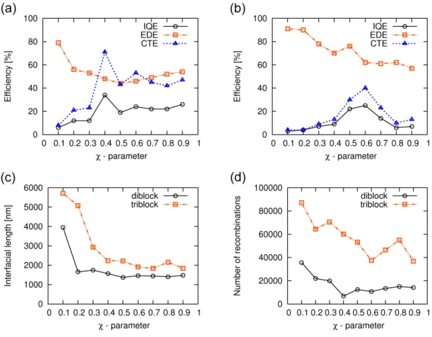
5 Investigation of loss phenomena of block-copolymer-based solar cells 50 5.1 Introduction . . . 51
5.2 Simulation details . . . 52
5.3 Simulation of block-copolymer-based solar cells . . . 53
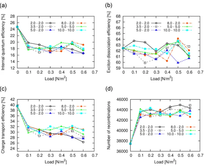
5.3.1 Effect of mechanical load on the photovoltaic performance . . . 61
5.3.2 Charge storage media . . . 63
6 Improving the solar-cell performance of polymer bulk heterojunctions 66 6.1 Introduction . . . 67
6.2 Dynamic-SCFT under the influence of an applied electric field for block-copolymers 68 6.3 Validation of the dynamic-SCFT method . . . 70
6.4 Simulation details . . . 70
6.5 Di- and triblock-copolymer melt under the influence of an electric field . . . 72
6.5.1 A5D15-diblock-copolymer melt . . . 72
6.5.2 A3D12A3-triblock-copolymer melt . . . 75
6.5.3 A3D12A3-triblock-copolymer systems in the presence of surface interactions 80 6.6 Influence of impurities on the photovoltaic efficiency . . . 83
7 Influence of chemical details on photovoltaic performance 86 7.1 Introduction . . . 87
7.2 Parameterized field-based approach and simulation parameters . . . 87
7.3 Application to lamellar-likeD10A10-homopolymer blend . . . 91
7.3.1 Influence of intermixing of theD- andA-components on the device efficiency 91 7.3.2 Comparison of current densities . . . 93
7.3.3 The effect of photo-oxidation on photovoltaic performance . . . 95
8 Full device calculations of polymer-based solar cells 97
8.1 Introduction . . . 98
8.2 Modified transfer-matrix method for bulk heterojunctions . . . 99
8.3 Simulation details . . . 100
8.4 Results . . . 101
9 Summary and conclusions 106
Appendices 111
A Supporting material to chapter 5 111
B Supporting material to chapter 6 120
References 121
Introduction
1.1 Organic electronics
Organic devices have attracted considerable attention in the past decade due to their great perspective in light weight, flexible and large area applications and the low fabrication costs [1, 2]. There are many different fields, in which they might be competitive with silicon technol- ogy, increasing their suitability for commercial applications [1] and, thus, their value for modern societies, like in the field of energy, information and communication [3]. Examples of organic electronic devices include organic thin-film transistors (OTFT), organic light-emitting diodes (OLED), organic photovoltaics (OPV), radio-frequency identification (RFID), nano-capacitors, sensors, memories, and more [1, 3]. The number of applications continue to grow as the tech- nology mature and as the global challenges require more sophisticated electronic devices. For instance, the OPV technology has generated significant interest in the last few years, due to the foreseeable shortage of fossil fuels as well as the necessity of limitingCO2 emission [4]. However, it is worth noting that the OPV devices differ substantially from their inorganic counterparts in their operation principles, as well as in their methods of production [4]. A major advantage of OPVs is that they can be fabricated using simple and low-cost production procedures, such as spin-coating, evaporation and printing techniques [3]. Moreover, their light weight and me- chanical flexibility confer them the potential to be easily integrable within consumer electronic devices, as illustrated in Fig. 1.1 [2, 4]. For this purpose, technologies such as roll-to-roll print- ing or spray coating technique, have recently been devised and prove to be useful for depositing OPV materials on various kind of substrates such as plastic, glass and others [3].
4
(a) (b)
Figure 1.1: (a) Organic solar cell printed on a flexible plastic substrate (reproduced from [4]).
(b) Plastic solar panel integrated into a bag for powering consumer electronic devices (Neuber’s Energy Sun-Bag).
1.2 Organic solar cells: problems and perspectives
Converting solar energy into electricity is one of the most important research challenges nowadays. Good efficiencies have already been achieved by using inorganic solar cells. For instance, an efficiency of 25 % has been realized with crystalline silicon solar cells, while a five junction cell of GaAs/InP has provided a value of 38.8 % [5]. However, a problem of latter examples is that they are very expensive in terms of both materials and techniques [6]. As an alternative, organic-based photovoltaics represent a potentially cheap and easily handable technology. Unfortunately, to this day the efficiency of OPV cells is still significantly lower compared to inorganic PV cells [6]. In order to enhance their performance, new materials with low band gap and device architectures have to be developed. The low power conversion efficiencies are mainly attributed to loss phenomena occurring during the photovoltaic process, such as photon loss, exciton loss and charge-carrier loss [7].
Nowadays, a large variety of experimental tools are available for characterizing the structure and measuring the efficiency of OPV devices. For instance, the grazing incidence X-ray scattering (GIXS), to characterize the morphology of the active layer, in combination with space-charge limited-current-measurement technique, to characterize the charge transport in the device, can provide useful information about morphology and electronic structure of polymer molecules in bulk heterojunction solar cells [8]. Another technique, the time-resolved electrostatic force microscopy (EFM) enables the measurement of photoexcited charge creation in organic thin
films with a spatial resolution better than 100 nm [132]. These results have been found to correlate with the external quantum efficiencies (EQE), in case of a series of polymer blends, composed of poly(9,9dioctylfluorene-co-bis-N,N-(4-butylphenyl)-bis-N,N-phenyl-1,4-phenylene- diamide) PFB and poly(9,9-dioctyl-co-benzo- thiadiazole) F8BT [132]. Moreover, it has been concluded from these experimental investigations that the domain composition of the PFB- and F8BT-phases is of crucial importance for optimizing charge-carrier transport and recombination rates within these domains. Thus, we see that, obtaining more detailed information about the local morphological characteristics of the active layer can help to improve the performance of OPV devices. However, experimentally it is difficult to distinguish between the different loss phenomena occurring during the photovoltaic process and to assess the impact of morphology and chemical details on them [118]. In this regard computer simulation techniques can contribute to a better understanding of the physical processes underlying the operation of OPV devices and support experimental investigations.
A first attempt to gain some insight into the relationship between the device morphology of an organic bulk heterojunction solar cell and its internal quantum efficiency (IQE) has been made by Watkinset al. [121], who proposed a dynamic Monte Carlo (DMC) model that treats exciton diffusion and charge transport in mixed donor/acceptor (D/A) structures. They have considered both disordered and ordered morphologies with different scale of phase separation and found that at an intermediate scale of phase separation a peak in the IQE is observed, which relates to an ideal compromise between exciton dissociation and charge transport. Moreover, they showed that the ordered checkered morphology exhibits a peak IQE, which is 1.5 times higher than the one of the disordered blend. In a subsequent work, Marsh et al. [118] have developed a DMC model, which enables to simulate dark injections at the electrodes. In this model they focused on the situation of charge separation and transport processes in organic nanostructures, but did not consider the exciton diffusion to the heterojunction. In other works, Meng et al. [60] and Kimber et al. [41] designed DMC models where they took into account all the microscopic photovoltaic processes, including the description of exciton behavior, charge transport as well as dark current injections. Moreover, Yang et al. [9] have proposed a DMC model, which includes in addition the effects of optical interference, to study the influence of the nanostructure on the solar cell efficiency of a device composed of copper phthalocyanine (CuPc) and C60. To calculate the distribution of exciton creations inside the device, i.e. the optical absorption distribution, they used the transfer-matrix method. This enabled them to calculate the absorption efficiencies for a series of heterojunctions and, thus, to evaluate their EQE’s, which were in good agreement with experimentally measured values. A similar DMC model has also been employed by Yan et al. [116], to investigate the influence of annealing on the device performance of PFB/F8BT bilayers. They found that with increasing annealing temperature the device performance systematically decreases, which was mainly attributed to a deteriorated separation probability of interfacial electron-hole pairs due to an increased disorder at theD/A
interface. However, the main drawback of these approaches is that the underlying techniques used for morphological generation, such as the Ising model in conjunction with Kawasaki spin- exchange dynamics or the techniques for generating idealized morphologies [41, 60, 121], do not rely on realistic polymer models and, therefore, do not allow to introduce chemical details.
A standard approach to describe a complex polymer system in a realistic fashion by com- putational means is to use the molecular dynamics (MD) simulation technique at atomistic resolution. However, with this technique we can only consider relatively small systems with up to 106 atoms in the nanosecond up to sub-microsecond time range. In order to cope with the structural-dynamical evolution of large-scale polymer systems with up to several million of atoms the transformation from the conventional particle representation to field representation can be performed by using the Hubbard-Stratonovich transformation [77, 81]. For polymers the resulting field-theoretic partition function integral can effectively be approximated by the mean-field (MF) approximation. For instance, Buxton and Clarke, in order to predict the mor- phologies of a diblock-copolymer system, used the Flory-Huggins Cahn-Hilliard model, which relies on the MF approximation [10]. To simulate the photovoltaic response of their devices, they utilized a two-dimensional drift-diffusion method. However, despite the low computational expense, this approach remains rather limited because it does not allow the explicit description of local particle processes, such as loss processes through charge recombination or accumulation at bottlenecks and dead-ends of the morphology. First achievements to overcome this problem have been realized in our previous work [69], where we developed a new multiscale algorithm to simulate the photovoltaic performance ofDA-polymer blends, which makes use of either the time-dependent Ginzburg-Landau method (TDGL) or the self-consistent field theory (SCFT), to generate the morphologies, in conjunction with the DMC method, to mimic the elementary photovoltaic processes. In another work [115], which was carried out in our group, we intro- duced a new particle-based multiscale solar-cell algorithm, to take into account the chemical nature of the monomers quantum mechanically. This permitted us to study the influence of photodegradation of the F8BT monomers on the photovoltaic performance of PFB/F8BT-blend devices. Moreover, by comparing its results with the ones of a field-based solar cell algorithm, we have estimated the influence of the local segmental composition and chemical defects on the local photovoltaic properties ofDA-polymer solar cells [115].
1.3 Scope of the thesis
The goal of this thesis is to develop and apply field-based multiscale modeling techniques, to better understand and improve the performance of nanodevices, used in optoelectronic applica- tions. For this purpose, we will use the SCFT technique, to compute the polymeric morphologies, in combination with a suitable DMC algorithm, to simulate the photovoltaic processes. The ap-
plication of this coupled multiscale approach will enable us to treat a large variety of polymer systems of large system size at low computational costs. To investigate the causes affecting the loss processes of elementary particles in block-copolymer systems with changing chemical characteristics and external conditions, such as the mechanical load, we will apply this DMC- SCFT method on systems composed ofDA-diblock- and ADA-triblock-copolymers. Moreover, we will investigate the suitability of these polymer systems for the use as charge storage media by analyzing their charge storage capacity as well as charge loading/unloading behavior. To elucidate the external parameters influencing solar-cell efficiency, we will analyze the impact of post-production techniques, such as electric-field alignment and surface interaction optimiza- tion, on the photovoltaic performance of polymer solar cell (PSC) nanodevices. Furthermore, we will study the influence of impurity particles, which might result from the diffusion of electrode material into the active layer, on the stability and performance of diblock-copolymer solar cells.
To investigate the effect of mixing of theD- andA-components on the exciton-dissociation and charge-transport efficiencies, we will extend our conventional DMC-SCFT approach, where the effect of mixing of the D- and A-components has been neglected, by introducing the compo- sition dependence of the exciton-dissociation frequency and charge-transfer integrals into the algorithm. The new method will be called the parameterized field-based multiscale solar-cell algorithm. In addition, to evaluate the influence of chemical changes through degradation of the polymer structure on the efficiency of PSCs, we will perform parameterized field-based cal- culations by taking into account the effect of photo-oxidation of the fluorene moieties. Finally, to investigate the impact of the architecture and composition of the full nanodevice on its ab- sorption efficiency and EQE, we will combine the parameterized field-based solar-cell algorithm with a modified version of the transfer-matrix method, which is used to determine the optical absorption distribution within the photoactive layer. The new method will be called the bulk heterojunction transfer matrix(BTM)-DMC-SCFT, which will enable us to take into account all major effects, affecting the performance of full nanodevices at moderate computational costs.
To attain these goals, this thesis has been organized in the following way. In Chapter 2, the SCFT technique is introduced, whereas in Chapter 3 an overview of basic working principles of organic solar cells as well as theories, describing the creation and transport of the elementary particles within the active layer of organic solar cells, is presented. In Chapter 4 a detailed description of the DMC algorithm is provided. Next, in Chapter 5 the loss phenomena of block-copolymer-based solar cells as well as their suitability to be used as charge storage media, are discussed in detail. Afterwards, in Chapter 6 possible ways for improving the photovoltaic performance as well as the influence of impurity particles on the stability and efficiency of polymer bulk heterojunctions are analyzed, whereas in Chapter 7 the influence of chemical details on photovoltaic performance is investigated. In Chapter 8 the results of full device calculations of polymer-based solar cells are presented and the thesis is completed with a summary and conclusions in Chapter 9.
Self-consistent field theory
9
2.1 Ideal chain models
In this chapter we introduce the SCFT for computing the polymeric morphologies used within this thesis. In ideal chain models only short-range interactions are taken into account.
Regardless of their particular form, all ideal chain models exhibit universal scaling properties [11]. One of the simplest ideal chain models is the lattice model, depicted in Fig. 2.1 (a). In this model a polymer chain is described by a set of inter-linked monomers, which are placed sequentially on the spatial lattice [12]. It is assumed that the lattice has a lattice constantb0.
b0
monomer
(a) (b)
rN
r
R
Figure 2.1: (a) Lattice model of polymers. (b) End-to-end vector (R) of a polymer chain.
One of the measures of the average size of a polymer chain can be characterized by the length of the vectorRbetween two end monomers of the chain (see Fig. 2.1 (b)). The average end-to-end distance of an ideal or Gaussian chain scales with the degree of polymerizationN as:
rD
|R|2E
= rD
|rN−r|2E
=b0Nν, ν= 1/2, N → ∞, (2.1)
where each bond connecting the monomers is assumed to have a lengthb0, whereasν is a univer- sal scaling exponent. The universality means that it does not depend on the chemical structure of the polymer chain and the level of coarse-graining. It is possible to show that the probability distribution of the end-to-end vector obeys the Gaussian distribution [12]:
P(R) = 3
2πN b20 3/2
exp −3|R|2 2N b20
!
. (2.2)
Another important class of ideal chain models is a bead-spring model, which is a useful start- ing point for studying the physical properties of polymers on large scales. The transformation
from lattice model to the bead-spring model can be done by grouping several monomers into larger units. The procedure, where the number of units is reduced from N monomers down to M segments is referred to as coarse-graining [14]. In such a way we are eliminating the infor- mation concerning microscopic degrees of freedom. When we define the coarse-grained segment the model parameters change asN →N/m =M and b =√
mb0. An important characteristic of the bead-spring model is that the probability distribution of the end-to-end vector of the coarse-grained polymer chain also obeys the Gaussian distribution, similar to Eq. (2.2). In statistics, this property is known as the central limiting theorem, which states that a sum of any large number of independent random variables tends to obey the Gaussian distribution [12, 14].
b
3kBT b2 spring constant
Figure 2.2: Bead-spring model.
In the bead-spring model the particles along the coarse-grained chain are considered to be connected by a harmonic spring (see Fig. 2.2), whose potential energy is given by [11, 12, 13]:
Ubond(b) = 3kBT
2b2 |b|2, (2.3)
whereb is a bond vector,kB is Boltzmann’s constant andT the system temperature. Since the spring constant depends on the temperature, the parameterbin this potential can be interpreted as an average of the square of the bond length:
D
|b|2E
=
R db|b|2exp [−βUbond(b)]
Rdbexp [−βUbond(b)] =b2, (2.4)
and, thus,b can be identified as the average bond length between the coarse-grained segments or the effective bond length.
Now, if we consider a linear chain composed of N + 1 segments connected by the above mentioned bond potential, the Hamiltonian of this polymer chain can be written as [12]:
H = 3kBT 2b2
N−1
X
i=0
|ri−ri+1|2+W(r,r, ...,rN)≡H0+W, (2.5)
whereri is a position vector of the i-th segment. The term denoted byH0 is the Hamiltonian of an ideal chain, whereas the termW is the interaction potential, which depends on the chain conformation, including interactions between the segments or the effects of an external field.
2.2 Ideal chain statistics
As was already mentioned previously, in ideal chain models only the effects of segment con- nectivity are taken into account. In other words, an ideal chain has no long-range interactions between the segments. In this case, the Hamiltonian of the bead-spring model of the ideal chain is given by the first term of the right hand side of the Eq. (2.5) [12]:
H=H0 = 3kBT 2b2
N−1
X
i=0
|ri−ri+1|2. (2.6)
By using the canonical ensemble, where the total number of particles (N), the total volume (V) and the temperature (T) of the system are fixed, the probability of finding the conformation {r, ...,rN}of the ideal chain is defined as [12]:
P({ri}) = 1 Z0
exp(−βH0) = 1 Z0
exp − 3 2b2
N−1
X
i=0
|ri−ri+1|2
!
, (2.7)
whereZ0 is a partition function of the chain
Z0 = Z
dr...
Z
drNexp[−βH0(r, ...,rN)]. (2.8)
After having performed the integration using the variable transformation from the position vec- tors {ri} to the bond vectors {bi} and the formula for the Gaussian integral, we obtain the following quantity ofZ0:
Z0 =V
2πb2 3
3N/2
, (2.9)
which defines the total number of possible conformations of an ideal chain composed ofN + 1 segments confined in a box with the volumeV.
2.3 Path-integral formalism for an ideal chain
The distribution function of the chain conformation in Eq. (2.7) is a function in 3(N + 1)- dimensional configuration space. By using the path-integral formalism, it is possible to rewrite this function in a more tractable form. For the sake of simplicity, it is convenient to start from the lattice model of the polymer chain. In order to calculate the statistical weight, we consider a subchain, which is a part of the whole Gaussian chain. The end segments of this subchain, specified by the indicesi0andi, are fixed at the sitesr0andr, respectively. The statistical weight of this subchain is defined asQ(i0,r0;i,r) and, due to the connectivity, relates toQ(i0,r0;i+ 1,r) through the following recurrence formula [15]:
Q(i0,r0;i+ 1,r) = 1 z
X
r00
Q(i0,r0;i,r00), (2.10)
wherez is a number of nearest neighbor sites and for a three dimensional latticez= 6, whereas r00 is one of the possible positions of the nearest neighbor sites to r.
By going from the discretized expression of Eq. (2.10) to a continuum formula, we have to subtractQ(i0,r0;i,r) from both sides of Eq. (2.10), to obtain the following expression:
Q(i0,r0;i+ 1,r)−Q(i0,r0;i,r) = 1 z
X
r00
Q(i0,r0;i,r00)−Q(i0,r0;i,r). (2.11)
By afterwards taking the continuum limit, where ∆i→ 0, the left hand side of Eq. (2.11) be- comes a derivative ofQ(i0,r0;i,r) and the right hand side of Eq. (2.11) becomes the Laplacian.
Then, replacing the discrete index iby a continuous parameters and taking the limit ∆s→0, Eq. (2.11) reduces to the three dimensional diffusion equation [15]:
∂
∂sQ(s0,r0;s,r) = b20
6∇2Q(s0,r0;s,r), (2.12) where the parameterscorresponds to time and the factor before the Laplacian can be regarded as the diffusion constantD=b20/6.
The solution of Eq. (2.12) under the initial condition that the end segment is fixed at the positionr0, is given by:
Q(s0,r0;s,r) =
3
2π|s−s0|b20 3/2
exp
−3|r−r0|2 2|s−s0|b20
, (2.13)
which again proves that the ideal chain obeys Gaussian statistics [15].
2.4 The mean-field approximation
If a polymer chain possesses strong segment-segment interactions between different type of segments or segment-object interactions, the polymer chain is no longer an ideal Gaussian chain [15]. In such a situation we have to take into account the interaction term W in the Hamiltonian in Eq. (2.5). Due to the nonlinearity of this term, the probability distribution of the chain conformation can no longer be calculated exactly and we have to rely on the approximate theory [12], which is in our case the mean-field theory.
In a polymer melt, the interaction between segments is screened out as a result of both the incompressibility condition and the ability of polymer chains to interpenetrate one another.
Due to the screening effect, the segment density fluctuations among the polymer chains are suppressed and each polymer chain in the polymer melt obeys ideal chain statistics. Mean-field approximation assumes that the correlations between a single chain, which is referred to as a tagged chain, and the other chains are neglected. Under this assumption, the conformation of the tagged chain can be approximated as an ideal chain in an external mean fieldV(r) generated by the surrounding polymer chains (see Fig. 2.3 (b)).
V (r)
tagged chain
(a) (b)
Figure 2.3: (a) An interacting many-chain system; (b) An ideal single chain in an external mean fieldV(r) generated by the surrounding polymer chains.
By considering the system composed of several species, the mean-field acting on the tagged segment at positionris given by [12]:
VK(r) =kBTX
K0
χKK0φK0(r) +γ(r), (2.14)
where χKK0 is the Flory-Huggins interaction parameter between K- and K0-type segments, φK0(r) is the volume fraction of K-type segments at position r, whereas γ(r) is the constraint force due to external conditions.
In the next section we will describe the technique, which is used to calculate the equilibrium conformation of the tagged chain in an average external potential field.
2.5 Path-integral formalism for a chain in a mean field
In the mean-field approximation, which is also known as self-consistent field theory (SCFT), the conformations of the tagged chain are evaluated with the use of the path-integral technique, where the segment-segment and segment-object interactions are treated as external fields, acting on the ideal Gaussian chain [15].
...
k r
r
00l − 1 l r
0Figure 2.4: Subchain representation for the path-integral formalism. The subchain is splitted into two parts for the purpose of derivation of a recurrence formula.
As in section 2.3, we focus on the subchain, which is assumed to be in equilibrium in the self-consistent fieldV(r) (see Fig. 2.4), whose end segments are specified by the indiceskand l and are fixed at positionsrand r0, respectively. The whole polymer chain composed ofK-type segments with indices (0, ..., N). When we substitute the interaction between the tagged seg- ment and the self-consistent field (Eq. (2.14)) instead ofW in Eq. (2.5), then the Hamiltonian of this subchain is given by:
H=H0+W = 3kBT 2b2
l−1
X
i=k
|ri−ri+1|2+
l
X
i=k
VK(ri). (2.15)
The Boltzmann factor of this Hamiltonian defines the statistical weight of the subchain, having a certain conformation, and is given by:
exp(−βH) = exp
"
− 3 2b2
l−1
X
i=k
|ri−ri+1|2−β
l
X
i=k
VK(ri)
#
. (2.16)
If both ends of the subchain are fixed at positions r and r0, the total statistical weight can be
expressed in path-integral form as [12]:
QK(k,r;l,r0)≡ V Z0(|l−k|)
Xexp
"
− 3 2b2
l−1
X
i=k
|ri−ri+1|2−β
l
X
i=k
VK(ri)
#
, (2.17)
where the sum is taken over all possible conformations, which satisfy the condition thatrk =r andrl=r0, whereas V is the volume of the system, which accounts for the translational degree of freedom of the center of mass of the chain. Moreover, Z0(|l−k|) is the partition function defined in Eq. (2.9), which represents the total number of possible conformations realized by an ideal subchain composed of|l−k|segments. By means of a Chapman-Kolmogorov relation:
QK(s,r;s0,r0) = Z
dr00QK(s,r;s00,r00)QK(s00,r00;s0,r0), (2.18)
which shows that the conformations of the subchains that have no common segments are statis- tically independent, it is possible to rewrite Eq. (2.17) in a more tractable form as a recurrence formula [12]. For this purpose, the subchain has to be splitted into two parts (see Fig. 2.4), where the last segment is treated separately from the other segments (i.e., i= k, ..., l−1 and i=l−1, l). As a result, Eq. (2.17) takes the form:
QK(k,r;l,r0) = V Z0(1)
Z
dr00QK(k,r;l−1,r00) exp
− 3
2b2|r00−r0|2−βVK(r0)
. (2.19)
After series of mathematical manipulations and integration, by taking a continuum limit of the discrete Gaussian chain model, where the discrete index i has been replaced by a continuous parameters, and the limit ∆s→0, we finally can write the following equation, which is called the Edwards equation [12, 15, 16]:
∂
∂sQ(s0,r0;s,r) = b2
6∇2−βVK(r)
Q(s0,r0;s,r). (2.20)
Due to the term containing VK(r), this is no longer a simple diffusion equation as Eq. (2.12), but it is a basic equation for calculating the path-integral.
In the next section we will made use of the continuous Gaussian chain model, to describe a general procedure for the SCFT method on the example of a diblock-copolymer melt. It is important to note, that in the continuous Gaussian chain model the polymer chain is viewed as a continuous Gaussian filament and obeys the same Gaussian statistics as the discrete bead-spring model [11]. Besides, the advantage of this model is that it allows calculations to be performed with partial differential equations, such as Eq. (2.20) [11].
2.6 General SCFT procedure
Up to now, we have been discussing a derivation of the general equations of the SCFT. In this section, we briefly review the SCF theory for a melt composed of AD-diblock copolymers [7, 16], for which, due to the screening effect between the monomers, we can assume Gaussian statistics for the chain conformation. Within this approximation, each polymer chain consists ofNA segments ofA-type andND segments ofD-type with their respective statistical segment lengths bA and bD, which means that the total number of statistical segments of a chain is N = NA+ND. To distinguish each segment, we consider that the configuration of the α-th chain can be described by a space curve rα(s) parameterized by the chain contour variable s, where the ranges 0≤s≤NA andNA≤s≤N describe, respectively, the A-block and D-block withs= 0 as the free end of theA-block ands=N as the other free end of theD-block (see Fig.
2.5). Let us next define the partition function integralQ(s0,r0;s,r), representing the equilibrium
r
α(0) 0
r
α(s) s
r
α(N ) N
Figure 2.5: The continuous Gaussian chain model.
statistical weight of a subchain between thesth- and s0th-segment with 0≤s0≤s≤N that is fixed at the positions r and r0. This statistical weight can be evaluated within the mean-field approximation by solving the following diffusion-type partial differential equation [7]:
∂
∂sQ(s0,r0;s,r) =
hb2
6∇2−βVA(r)i
Q(s0,r0;s,r), 0≤s≤NA, hb2
6∇2−βVD(r) i
Q(s0,r0;s,r), NA≤s≤N, (2.21) whereβ = 1/(kBT) and VA(r) as well asVD(r) are external potentials, acting on A- orD-type segments at positionr. The latter functions represent mean-field potentials, resulting from the interaction between the segments as well as from enforcing the incompressibility condition, and are obtained in a self-consistent fashion. Moreover, the initial condition for Eq. (2.21) is given byQ(0,r0; 0,r) =δ(r−r0). Because the two ends of the block copolymer are not equivalent, we need to introduce an additional statistical weight Q∗(s0,r0;s,r), which is calculated in the op- posite direction along the chain starting from the free ends=N. To reduce the computational
expense, the integrated statistical weights are defined in the following as:
q(s,r) =R
dr0Q(0,r0;s,r), q∗(s,r) =R
dr0Q∗(0,r0;s,r). (2.22)
These latter weights can be proven to satisfy Eq. (2.21) similarly as the non-integrated ones.
This then leads to the following diffusion equation:
∂
∂sq(s,r) =
hb2
6∇2−βVA(r)i
q(s,r), 0≤s≤NA, hb2
6∇2−βVD(r) i
q(s,r), NA≤s≤N, (2.23)
with the initial conditionq(0,r) = 1. Analogous expressions can be formulated for q∗(s,r). By using the definitions in Eqs. (2.22), the volume fractions of the A- and D-type segments at positionrcan be written as:
φA(r) =C Z NA
0
dsq(s,r)q∗(N −s,r), (2.24)
φD(r) =C Z N
NA
dsq(s,r)q∗(N −s,r), (2.25)
where the normalization constant in the canonical ensemble is given by:
C = V
R drR
dsq(s,r)q∗(N −s,r) = V
N Z, (2.26)
with V as the total volume of the system and Z as the single-chain partition function. The external potentialVK(r) of aK-type segment (K =A orD) can be decomposed into two terms in the following way [7]:
VK(r) =X
K0
KK0φK0(r)−µK(r) =WK(r)−µK(r), (2.27)
where the first term represents the interaction energy between the segments with KK0 as the nearest-neighbor pair-interaction energy between a K-type and K0-type segment. The latter quantity is related to the Flory-Huggins interaction parameter through the following expression χAD =Nnsβ[AD(1/2)(AA+DD)], where Nns is the number of nearest-neighbor sites. More- over, the function µK(r) is the chemical potential of the K-type segment, which represents a
Lagrange multiplier that enforces a constraint imposed on the system, such as the incompressibil- ity condition. To obtain the volume fractions of the equilibrium nanostructured morphologies, the previous system of equations has to be solved in an iterative manner. First of all, the po- tential fields VA(r) and VD(r) are determined from the volume fractions φA(r) and φD(r) by making use of Eq. (2.27). Afterwards, the weightsq(s,r) and q∗(s,r) are calculated by solving Eqs. (2.23) that contain the fields VA(r) and VD(r). Finally, the new volume fractions φA(r) and φD(r) are calculated from the weights q(s,r) andq∗(s,r) through Eqs. (2.24) and (2.25).
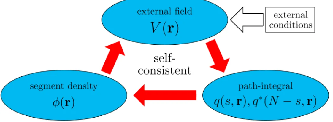
The procedure is repeated until a self-consistent solution is reached. In Fig. 2.6 we show the basic scheme of the SCF theory.
After the self-consistent solution is obtained, the Helmholtz free energy of the system can be external field
V (r)
path-integral
q(s, r), q
∗(N − s, r)
segment density
φ(r)
self- consistent
external conditions
Figure 2.6: The basic scheme of the iterative procedure of the SCFT.
calculated as follows:
F =−kBT MKlnZ+1 2
X
K
X
K0
Z
drKK0φK(r)φK0(r)−X
K
Z
drVK(r)φK(r), (2.28)
whereMKis a total number ofK-type chains in the system. This quantity relates to the average number density ofK-type segments ¯φK through the equation:
MK = Vφ¯K
NK+ 1, (2.29)
whereV is the system volume andNK is the total number ofK-type segments.
2.6.1 Static calculation
In order to get the equilibrium state in the static SCF calculation, the two fieldsWK(r) and µK(r) in Eq. (2.27) are updated simultaneously, according to the following iterative scheme:
WK(r)→WK(r) +αW (
X
K0
KK0φK0(r)−WK(r) )
, (2.30)
µK(r) =µK(r)−αV
(
1−X
K
φK(r) )
, (2.31)
whereαW andαV are appropriately chosen constants between 0 and 1. By introducing updated WK(r) and µK(r) into Eq. (2.27), the path-integral is recalculated. The iteration procedure, illustrated in Fig. 2.6, is repeated until the fields are converged and the incompressibility condition is fulfilled within a certain error [15, 17].
2.6.2 Dynamic calculation
The dynamical mean-field method is based on the diffusion dynamics of the segments. As- suming Fick’s law of linear diffusion and combining it with the conservation law for the segment density, which is expressed by the continuity equation, the time-evolution equation for the seg- ment density can be written as follows [12, 15, 17]:
∂
∂tφK(r, t) =∇ ·[LK(r, t){∇µK(r, t) +λ(r, t)}] +ξK(r, t), (2.32)
whereLK(r, t) is a mobility of the K-type segment and λ(r, t) is a Lagrange multiplier for the local incompressibility condition. Moreover, ξK(r, t) is a random noise due to thermal fluctua- tions, satisfying the following fluctuation-dissipation relation:
ξK(r, t)ξK0(r0, t0)
= 2kBTLKK0(r, t)∇2δ(r−r0)δ(t−t0), (2.33)
whereLKK0(r, t) is given by the local mobility coefficient LK(r, t) as:
LKK0(r, t) =LK(r, t)δKK0 +LK(r, t)LK0(r, t) P
K00LK00(r, t) . (2.34) The segment density distribution profiles {φK(r)} are obtained by the integration of the time-evolution equation. In the next time step, the chemical potential µK(r) is evaluated from the given segment density distribution φtargetK (r). After the initialization of WK(r) and µK(r)
with 0, the following iteration scheme is used [17]:
WK(r)→WK(r) +αW n
WKtarget(r)−WK(r) o
, (2.35)
µK(r) =µK(r)−αV
n
φtargetK (r)−φK(r) o
, (2.36)
whereWKtarget(r) =P
K0KK0φtargetK0 (r). This procedure is repeated untilWK(r) andµK(r) have converged within a certain error.
Theoretical background for organic photovoltaics
22
3.1 Basic working principles of organic solar cells
3.1.1 Brief history
One of the first reported investigations about organic (excitonic) photovoltaic cells dates back to 1959, when Kallman and Pope discovered that the single crystals of an anthracene can be used to produce the photo-voltage [18]. Despite an extremely low efficiency of 0.1 %, this discovery gave a boost to subsequent years of research. Attempts to improve the efficiency of a single-layer organic solar cells were unsuccessful, mainly due to the reason that strongly bound excitons were formed, which are difficult to split into free charges, in order to produce a current.
The next breakthrough in the field of OPVs was done by Tang in the mid eighties, when he introduced the concept of a bilayer heterojunction and demonstrated relatively high efficiencies of around∼1 % [19, 20]. In this concept an electron donor material (D) and an electron acceptor material (A) were brought together and sandwiched between the electrodes. The interface between these two thin organic layers played a critical role in determining the photovoltaic properties. The improved efficiency resulted from the increased exciton dissociation at the planar D/Ainterface, which relates to the different electron affinities of the two materials. After a fast process of charge transfer and spatial separation of the electron and hole, the charges are able to migrate towards their respective electrodes to generate a photocurrent. The main limitation of the two-layer OPV cells is that the exciton diffusion length in organic semiconductors is typically less than 10 nm, which causes that a large number of excitons are lost on the way to the heterojunction [18, 19]. However, for the effective absorption of the incident light, a layer thickness of the absorbing material has to be much more than the diffusion length of the excitons. For this reason the device efficiencies for many years were limited to around∼1 %.
To overcome the problem with exciton diffusion length, Yu et al. [21] in 1995 proposed to mix conducting polymers with buckminsterfullerene, to obtain interpenetrating network of donor and acceptor materials. Such device structure is called a bulk heterojunction (BHJ).
For this system they reported a power conversion efficiency of about 2.9 %. The substantial enhancement in efficiency with the bicontinuous network material results from the large increase in the interfacial area, which causes the reduction in the distance the excitons have to travel to reach the interface [21]. The disadvantages of the BHJ are that it is more difficult to separate Coulomb bound charge-carrier pairs and that percolation paths to the electrodes are not always present, due to the increased disorder of the material [36].
Nevertheless, the concept of BHJ has become popular, which essentially relates to the fact that the power conversion efficiencies of organic BHJ solar cells over the last few decades have increased significantly from ∼ 1 % to more than 10 %, demonstrating their great potential in the field of cost-efficient photovoltaics [18, 29].
3.1.2 Organic solar cell architecture
A typical organic solar cell consists of at least five distinct layers, as depicted in Fig. 3.1.
Substrate IT O P EDOT :P SS
Aluminum
Active layer Conjugated polymers
PFB F8BT
Figure 3.1: Diagram of the architecture of a polymer solar cell. The active layer either consists of a bilayer or a blend of donor- and acceptor-polymers. The inset shows the chemical structures of donor- and acceptor-type polymers composed of PFB and F8BT, respectively.
One of the electrodes must be transparent, to allow the photoexcitation of the active materials.
The glass or plastic (some flexible transparent polymer) may be used as a substrate. Suitable substrates should fulfill following requirements [4]:
1. Low cost;
2. Chemical and thermal stability;
3. Mechanical and environmental stability;
4. High optical transparency.
Currently the most frequently used substrate is glass. Nevertheless, flexible plastic substrates have become popular in production of solution-processed organic photovoltaics, using roll-to- roll methods [4, 22]. As illustrated in Fig. 3.1, on top of the substrate is laid one of the
electrodes, which is a transparent conductive oxide, called indium-doped tin oxide (IT O). The IT O electrode is normally coated with a conducting polymer. The most commonly used ma- terial for this purpose is a mixture of poly(3,4-ethylenedioxythiophene):poly(styrene sulfonate) (P EDOT :P SS), which helps to smooth out the roughness ofIT O surface and to increase its work function [4]. Moreover, it serves as a hole transporter and exciton blocker [31]. Next, on top of the P EDOT :P SS the active layer is deposited, which either consists of a bilayer or a blend of donor- and acceptor-polymers. For instance, PFB and F8BT are donor- and acceptor- materials, commonly used. Their chemical structures are illustrated in Fig. 3.1. This layer is responsible for light absorption, exciton generation and dissociation at heterojunction with subsequent transport of the charge carriers to the respective electrodes [31]. Finally, the second electrode is put on top of the active layer, often with an additional very thin buffer layer (Ca or LiF, not shown in Fig. 3.1), which keeps electrode material (normally Al) from diffusing into the photoactive layer [18]. Both Al from the cathode and In from the anode can diffuse as impurities into the active layer, which can contribute to the degradation of the device [86]. This issue will be discussed in section 6.6.
3.1.3 The solar spectrum
To achieve a high efficiency, the solar cell needs to absorb a large portion of the light of the solar spectrum. The total power density received at the top of the Earth’s atmosphere is approximately 1360W m−2for the extraterrestrial spectrum [23]. When light is passing through the atmosphere, a large part of this energy is absorbed and scattered by different atmospheric constituents. In the infrared region of the spectrum the absorption is almost entirely caused by H2O (absorbs light at 900, 1100, 1400 and 1900 nm) andCO2 (absorbs light at 1800 and 2600 nm), as well as by dust, whereas in the ultraviolet region of the spectrum the light is cutted off by oxygen, ozone and nitrogen (light below 300 nm) [24].
The absorption increases with the length traveled within the atmosphere. In order to take into account the dependence of the light intensity on the optical path length through the atmo- sphere, a new term, called “Air Mass” (AMn), is introduced:
n= optical path length to the sun
optical path length when the sun is directly overhead = 1
cos(θ), (3.1)
where θ is the zenith angle in degrees. The spectrum outside the atmosphere is referred to as AM 0 and that on the surface of the Earth for normal incidence is referred to as AM 1 [24].
A typical solar spectrum at which solar cells are measured is AM 1.5, which corresponds to an angle of incidence of solar radiation of 48◦ relative to the surface normal [24]. The power density
received in this case is:
PAM1.5 = 1000W m−2. (3.2)
In Fig. 3.2, we show the AM 0 and AM 1.5 solar spectra, alongside with the black body spectrum for T = 5760 K. We deduce from the graph that the greatest solar irradiance is close to the visible range of wavelengths (300 - 800 nm).
Figure 3.2: American Society for Testing and Materials (ASTM). The extraterrestrial solar spectrum (AM 0), the terrestrial solar spectrum (AM 1.5) and the black body spectrum atT = 5760K (reproduced from [25, 37]).
It is clear that for the construction of an efficient device the absorption spectrum of the active layer must closely match the incident solar spectrum. A problem is that absorption of polymer blends strongly depends on the characteristics of their mesoscopic structure, precluding transferability among different experimental measurements. In section 4.4, we will introduce a transfer-matrix formalism to calculate the spatial distribution of absorbed power as a function of thickness and wavelength, depending on the optical constants of the respective nanophases in the active layer, which takes into account optical interference effects [137].
3.1.4 Operational principles
In a PSC the main fraction of the light is absorbed in the donor material. If a photon has an energy (hν) larger than the energy gap (Eg) of the material, the photon is absorbed. Upon photon absorption an electron in the organic semiconductor is excited from the highest occupied molecular orbital (HOMO) into the lowest unoccupied molecular orbital (LUMO) (see Fig. 3.3).
This has some analogy with the process of exciting an electron from the valence band to the conduction band in case of inorganic semiconductors [26]. However, due to the low dielectric constant of organic semiconductors (typically between 3 and 4), strong Coulomb attraction of an electron-hole pair leads to the creation of a bound electron-hole pair, which is called an exciton.
The created exciton diffuses and must reach a D/Ainterface within its lifetime to undergo the dissociation, otherwise it will recombine by emitting a photon or decay via thermalization (non- radiative recombination) [27, 28].
Energy
ITO
Al HOMO
LUMO
Donor
HOMO LUMO
Acceptor +
Eg -
+
-
- Voc
Figure 3.3: Schematic energy diagram of an organic heterojunction solar cell. The active layer consists of a donor and an acceptor material.
The exciton binding energy of organic semiconductors ranges between 0.1 and 1.4 eV, and is much higher compared to the ones of inorganic semiconductors with binding energies of a few meV [26]. Since their exciton binding energy exceeds the thermal energy at room temperature, the photogenerated excitons are only hardly separated into electrons and holes. To provide the necessary energetic driving force for charge separation, the energy offset between the LUMO of the donor and the acceptor (∆LUMO) should be greater than the exciton binding energy [29].
If this condition is fulfilled, the photoinduced charge transfer of the electron from the LUMO of the donor to the LUMO of the acceptor become energetically favorable. The positively charged hole remains on the donor material. This photoinduced charge transfer takes place at a time scale of ∼ 50 fs [26, 27]. The competing processes, like photoluminescence and
recombination of the charges, take place at much larger time scales, i.e. in the nanosecond and microsecond time ranges, respectively [27]. As a result, this allows efficient exciton dissociation at the heterojunction. Once the charges have been successfully separated, they have to travel to the respective electrodes within their lifetimes, where they are collected, contributing to a current in the external circuit. The potential difference of a high work function anode and low work function cathode creates a built-in electric field, which serves as a driving force for the charge transport within the PSC. During the charge transport throughout the bulk of the active layer, non-geminate recombination may occur between independently generated electrons and holes. This process is called bimolecular charge recombination.
The primary parameter, reflecting the charge transport properties of photovoltaic cells, is the external quantum efficiency (EQE), which is also called IPCE (Incident Photon to Current Efficiency). The EQE is defined as the number of electron-hole pairs flowing in the external circuit to the number of incident photons [30]:
ηEQE =ηA ·ηIQE, (3.3)
where ηA is the absorption efficiency, whereas ηIQE is the internal quantum efficiency (IQE), which considers only absorbed photons. Therefore, the IQE is defined as the number of carriers collected at the electrodes to the number of photons absorbed in the device [30, 31] and can be expressed as:
ηIQE =ηEDE ·ηCT E = (nge+ngh) 2ngex
· (nce+nch)
(nge+ngh) = (nce+nch) 2ngex
, (3.4)
whereηEDE andηCT E are the exciton dissociation and charge transport efficiencies, respectively.
In the previous equationnge,nceandngh,nchrepresent the number of electrons and holes generated in the bulk and collected at the electrodes respectively, whereas ngex represents the number of generated excitons. The factor of 2 in Eq. (3.4) accounts for the fact that the splitting of one exciton generates two charges [32].
3.1.5 Current-voltage characteristic
Current-voltage (I−V) characteristic under illumination is a common way to characterize the performance of organic photovoltaic cells. As illustrated in Fig. 3.4, in the dark the cell be- haves as a diode. At short-circuit condition, there is no current and at sufficiently large forward bias across the terminals the dark current is generated, resulting from carriers injected from the
electrodes. When the device is exposed to light, the incident photons generate a photocurrent and theI−V curve shifts downward (red solid line in Fig. 3.4). The current that flows through
I [A/m
2]
V [V]
ISC
VOC
MPP IM P P
VM P P
P out
Dark current Under illumination
Figure 3.4: Schematic current-voltage characteristic of a polymer solar cell under illumination (red solid line) and in the dark (dashed line). Circles on the graph indicate key points: ISC – the short-circuit current; VOC – the open-circuit voltage; MPP – the maximum power point; IM P P andVM P P are the values of photocurrent and voltage for which the output power is maximum.
the illuminated solar cell, when there is no external resistance (at zero applied voltage, V = 0 V), is called the short-circuit current (ISC). This is the maximum current that the cell is able to produce [31]. On the other hand, the maximum possible voltage (beyond which the solar cell no longer provides power) the photovoltaic cell can supply is the voltage, where the current under illumination is zero (I = 0 A/m2), and is termed open-circuit voltage (VOC). It is approximately limited by the energy offset between the HOMO of the donor and the LUMO of the acceptor (see Fig. 3.3) [28]. At any value of external load between theISC andVOC, the solar cell is doing work at a rateP =I·V, which defines the output power at the operating point [37]. The point where the magnitude of the product of photocurrent and voltage is maximum is designated as the max- imum power point (MPP), and the power at this point is equal toPout=IM P P·VM P P. The ratio between the maximum power output to its theoretical power output is called the fill factor (F F):
F F = IM P PVM P P
ISCVOC , (3.5)
which defines the squareness of the I−V curve. The F F also can be seen as an area ratio of the filled and unfilled rectangles (see Fig. 3.4). The above mentioned parameters can be used to
calculate the power conversion efficiency (P CE), which determines the percentage of the solar energy harvested by the cell that is converted into usable electrical power:
P CE= Pout Pin
= ISCVOCF F Pin
, (3.6)
where Pin is the incident light power radiated by the sun or by the standard instruments for solar-cell device testing [28].
3.2 Semiconducting polymers
Conventional polymers such as plastics, rubbers, etc., have substantial electrical resistance and are either insulators or very poor electrical conductors [33, 34]. However, with the discovery of the conductive properties of polyacetylene in the 1970s, polymers have received consider- able attention in the field of organic electronics [33]. They can either be semiconductors or conductors. From the band theory, it is well-established that the size of the energy band gap determines whether the polymer is a conductor, semiconductor or insulator [35]. The conduc- tivity in polymer-based semiconductors relates to conjugation, resulting from the alternation of single and double bonds between neighboring carbon atoms [36]. The overlap of thepz electron wavefunctions leads to delocalization and formation ofπ orbitals. Due to the Peierls instability, there are two delocalized energy bands: the bonding (π) and anti-bonding (π∗) orbitals [36].
The energy gap between the HOMO in the π-band and the LUMO in the π∗-band determines the semiconducting nature of the system [37]. Due to the amorphous nature of the polymers, the delocalization length of the π orbitals is limited to a definite conjugation length. This causes that the charges become localized on small segments of the polymer chain, which are called conjugated segments [37]. The random fluctuation in conjugation length of the polymer chains creates a disordered distribution of electronic states between segments. This energetic disorder can be approximated by the Gaussian density of states (DOS) [38]. Here, it should be noted, that excitons are also subjected to localization and energetic disorder but in a different way than charges [37]. An exciton is confined to a chromophore, which has a length of typically 5 monomers [39]. The energetic disorder of chromophores can also reasonably be approximated by the Gaussian distribution, as described in detail in Ref. [37].
3.3 Energy transport
3.3.1 Exciton formation
Let us now consider that an unexcited organic molecule, in which electronic spins are paired (opposite spins), is in the ground singlet state, S0. Upon photon absorption the molecule is excited and an electron is promoted from the S0 state into a new state of higher energy. If the transition occurs without change of spin, the new excited state is also a singlet state, S1, or higher excited singlet states Sn. The transition of an electron between states of unlike multiplicity (S1 → T1) is spin-forbidden and occurs only because of spin-orbit coupling, which allows for intersystem crossing. Due to the low dielectric constant of common organic materials (εr ∼ 3 - 4), Coulomb bound electron-hole pairs are created upon light absorption, which are called excitons. It has been shown by Narayan et al. [40] that singlet excitons diffuse and dissociate faster than triplet excitons at heterojunctions of organic solids, due to a lower binding energy.
Besides, because of higher diffusion coefficient, the singlet excitons have a higher diffusion length than the triplet excitons, which has been investigated using F¨orster and Dexter energy transfer models, respectively [40].
3.3.2 Exciton transport
The efficiency of the exciton dissociation process strongly depends on the exciton transport within the material of interest and is usually modeled using F¨orster resonance energy transfer theory (FRET) [42, 44]. FRET is a long-range mechanism and refers to the non-radiative energy transfer of an electronic excitation from a donor molecule to an acceptor molecule and does not require physical contact between them [45]:
D∗ + A →D + A∗
This energy transfer arises from a dipole-dipole interaction between the electronic states of the donor and the acceptor molecules. Since the energy must be conserved, the energy gain of the acceptor must be the same as the energy loss of the donor [43]. The rate of energy transfer, which was determined by F¨orster, is given by [43]:
ωET =ωer0
r 6
, (3.7)
whereωe= 1/τ0 withτ0 as the fluorescence lifetime of the exciton,r0 is the exciton localization radius (the F¨orster radius) andris the distance between donor and acceptor. The F¨orster radius


![Figure 4.2: Geometry of multilayer stack used for the optical electric field calculations [30]](https://thumb-eu.123doks.com/thumbv2/1library_info/5604374.1691193/51.892.273.658.139.630/figure-geometry-multilayer-stack-optical-electric-field-calculations.webp)