APPROXIMATIONS AND CONTAMINATION BOUNDS FOR PROBABILISTIC PROGRAMS
1Martin BRANDA and Jitka DUPA ˇCOV ´A
Charles University in Prague, Faculty of Mathematics and Physics, Depart- ment of Probability and Mathematical Statistics, Czech Republic
ABSTRACT:
In this paper we aim at output analysis with respect to changes of the proba- bility distribution for problems with probabilistic (chance) constraints. The perturbations are modeled via contamination of the initial probability dis- tribution. Dependence of the set of solutions on the probability distribution rules out the straightforward construction of the convexity-based global con- tamination bounds for the perturbed optimal value function whereas local results can be still obtained. To get global bounds we shall explore several approximations and reformulations of stochastic programs with probabilistic constraints by stochastic programs with suitably chosen recourse or penalty- type objectives and fixed constraints.
Key words: Stochastic programs with probabilistic constraints, output ana- lysis, contamination technique
AMC 2000: 90C15, 90C31, 90C29
1The paper is based on presentations held in APMOD 2008 in Bratislava, May 26 – 29, 2008.
1 Modeling issues
Classical stochastic programming (SP) models aim at hedging against con- sequences of possible realizations of random parameters — scenarios — so that the expected final outcome or position is the best possible.
Modeling part of realistic applications consists of a clear declaration of ran- dom factors to be taken into account, of distinguishing between hard and soft constraints and of a choice of a sensible optimality criterion. The starting point may be formulation of a deterministic problem which would be solved if no randomness is considered, e.g.
min{f(x) : x∈ X, gk(x)≤0, k = 1, . . . , m}.
Taking into account the presence of a random factor ω and the fact that a decision x has to be chosen before ω occurs, a reformulation of the minimi- zation problem is needed. Two prevailing approaches have been used to this purpose:
• static expected penalty models,
• probabilistic programs.
For penalty type models, X is defined by hard constraints plus some other conditions that guarantee plausible properties of the model, whereas soft constraints, such as gk(x, ω) ≤ 0, are reflected by penalties included into the random objective function. For probabilistic programs, probabilistic reliability-type constraints are introduced.
1.1 Stochastic programming models with penalties
The basic SP model with penalties is of the form
minx∈X EPf(x, ω). (1)
It is identified by
• a known probability distributionP of random parameter ω whose sup- port Ω is a closed subset of IRs; EP denotes the corresponding ex- pectation. In the sequel, the same character ω will be used both for the random vector and its realization.
• a given, nonempty, closed set X ⊂IRn of decisions x,
• a preselected random objective f fromX ×Ω to the extended reals — a loss or a cost caused by the decision x when scenario ω occurs. As a function of ω, f is measurable for each fixed x ∈ X and such that its expectationEPf(x, ω) is well defined. The structure off may be quite complicated e.g. for multistage problems. For convex X, a frequent assumption is that f is lower semicontinuous and convex with respect to x,i.e. f is convex normal integrand.
An example of (1) is the two-stage stochastic linear program with fixed re- course where X is convex polyhedral and the random objective function f(x, ω) =c>x+q(x, ω) involves the second-stage (recourse) function q defi- ned as
q(x, ω) = min
y {q>y : W y =b(ω)−T(ω)x, y ∈IRr+}. (2) Vector q ∈ IRr and recourse matrix W(m, r) are fixed, b(ω), T(ω) are of consistent dimensions with components affine linear in ω.
Our knowledge of probability distribution P is often merely a hypothesis.
Hence, we want to know, how sensitive to its violation our solution of (1) is.
To this purpose we shall consider F(x, P) := EPf(x, ω) as a function from X × P to extended reals, where P is a set of probability distributions on Ω.
This implies that in (1) X is independent of P.
1.2 Probabilistic constraints
Instead of (1) one may consider stochastic programs
x∈X(Pmin)F(x, P) :=EPf(x, ω) (3) in which the set of feasible solutions X(P)⊂IRn depends on the probability distribution P.
Formally, the independence of the set of feasible solutions of P can be achie- ved by means of the extended real indicator functions. Problem (3) can be e.g. written as
minx∈X
hF(x, P) + indX(P)(x)i (4) with X(P)⊂ X ⊆IRn, X a fixed closed set independent of P,and the indi- cator function indX(P)(x) := 0 for x ∈ X(P) and +∞ otherwise. However, the resulting extended real objective function in (4) is then very likely to lose the convenient properties of the original objective function F(x, P) in (3).
A special type of (3) is probabilistic programming obtained when X(P) = X ∩ Xε(P) withXε(P) defined e.g. by the joint probabilistic constraint
Xε(P) := {x∈IRn:P(g(x, ω)≤0)≥1−ε)} (5) with g : IRn×Ω → IRm and ε ∈ (0,1) fixed, chosen by the decision maker.
It is a reliability type constraint which can be written as H(x, P) := P( max
k=1,...,mgk(x, ω)≤0)≥1−ε. (6) We make use of the following convention: If V(ω) is a predicate on ω, we write P(V(ω)) instead of P({ω∈Ω :V(ω)}).
Individual, separate probability constraints are a special type of probabilistic constraints which treat constraintsgk(x, ω)≤0 separately: Given probability thresholds ε1, . . . , εm the feasible solutions arex∈ X that fulfilm individual (separate) probabilistic constraints
P(gk(x, ω)≤0)≥1−εk, k = 1, . . . , m. (7) This is a relatively easy structure of problem, namely, if ωk are separated being the right-hand sides of constraints, i.e. gk(x, ω) = ωk−gk(x)∀k.
Denoteu1−εk(Pk) quantile of marginal probability distributionPkofωk.Then (7) can be reformulated as
gk(x)≥u1−εk(Pk), k = 1, . . . , m.
For concave gk(x)∀k the set of feasible decisions is convex and for linear ob- jective function and lineargk(x)∀kthe resulting problem is a linear program.
Such results are no more valid for joint probability constraints. Even for ran- dom right-hand sides only, special requirements on the probability distribu- tion P are needed; cf. log-concave or quasiconcave probability distributions [28]. These seminal results on convexity properties of the set Xε(P) and of the related functionH(x, P) are due to Pr´ekopa; see e.g. [27, 28]. They have been reported and further extended in various monographs and collections devoted to stochastic programming, e.g. [2, 22].
Semicontinuity properties of the corresponding indicator functions, see e.g.
[21], can be obtained under various sets of assumptions about the function g and/or its componentsgk and about the probability distribution P.These
play an important role in qualitative and quantitative stability analysis with respect to changes of the probability measure; see [30].
Klein Haneveld [26] suggested to replace probability constraints (5) and (7) by Integrated Chance Constraints,ICC
EP(max
k [gk(x, ω)]+)≤β and EP([gk(x, ω)]+)≤βk∀k, (8) respectively, with fixed nonnegative valuesβ, βk.Mathematical properties of ICC are much nicer and from the modeling point of view, it is convenient that integrated chance constraints quantify the size of unfeasibilities.
The two prevailing types of static stochastic programs — with penalties and with probabilistic constraints — are not competitive but rather complemen- tary. Contrary to penalty models, probabilistic programs capture the relia- bility requirements or risk restrictions even in cases which do not allow for reasonably accurate evaluation of penalties, e.g. [15]. A suggestion of [28]
is to apply probabilistic constraints (5), (6) or (7) and at the same time, to extend the objective function for an expected penalty term which is active whenever the original constraints gk(x, ω)≤0 are not fulfilled:
Pr´ekopa [28] “...we are convinced that the best way of operating a stochastic system is to operate it with a prescribed (high) reliabi- lity and at the same time use penalties to punish discrepancies.”
In addition, ideas of multiobjective programming can be used if the choice of the penalty function is not clear and multiple penalty functions are therefore considered; cf. [29].
Another suggestion of [28] was to assign a probabilistic constraint on the second-stage variablesyin the two-stage stochastic program as a way how to restrict a possible unfeasibility of the second-stage constraints in incomplete recourse problems. Integrated chance constraints (8) of [26] aim at a similar goal.
Such extensions may be useful when modeling real problems. An example of a “mixed” model and its properties was recently presented in [3]; see Example 3.
In this paper we focus on potential applications of the contamination tech- nique to quantitative stability results for the optimal value of probabilistic programs with respect to changes in probability distribution P. The brief
presentation of the contamination technique in Section 2 reveals that its ex- ploitation to construction of global contamination bounds for probabilistic programs is limited. Therefore their reformulations to expected penalty-type problems are suggested in Section 3. As illustrated in Section 4, such refor- mulations open a possibility to construct approximate global contamination bounds for the probabilistic programs in question.
2 Contamination technique
In real applications, full knowledge of the probability distribution P can hardly be expected. Assume instead that the SP of interest, e.g. (9) was solved for a suitably chosen probability distribution P which is considered a sensible choice regarding the problem to be solved and the available input data. The first issue of interest is then the sensitivity of the obtained optimal solutions with respect to perturbances of the probability distribution. It may be quantified by bounds on the “error” in the perturbed optimal value. The background of relevant techniques is based on advanced results of parametric programming, e.g. [30].
We shall exploit parametric stability and sensitivity results, ideas of multi- objective optimization and the contamination technique to derive bounds for the perturbed optimal value function focusing on probabilistic programs and related problems. See [16] for discussion of the first results in this direction developed for stress testing of the risk measure VaR.
Contamination technique was initiated in mathematical statistics as one of the tools for analysis of robustness of estimators with respect to deviations from the assumed probability distribution and/or its parameters. It goes back to von Mises and the concepts are briefly described e.g. in [32]. In stochastic programming, it was developed in a series of papers, see e.g. [7, 10]
for results applicable to two-stage stochastic linear programs with recourse.
Describing perturbation by means of contamination occurs also in sensitivity analysis of worst-case probabilistic objectives with respect to deviations from the assumed type of probability distributions, cf. [25].
For derivation of contamination bounds one mostly assumes that the sto- chastic program is reformulated as
minx∈X F(x, P) := EPf(x, ω) =
Z
Ω
f(x, ω)P(dω) (9)
where P is a fixed fully specified probability distribution of the random pa- rameter ω ∈ Ω ⊂ IRs, X ⊂ IRn is nonempty, closed, independent of P and f : IRn×IRs→IR such that the expectation EP is well defined.
Denoteϕ(P) the optimal value and X∗(P) the set of optimal solutions of (9).
Possible changes or perturbations of probability distribution P are modeled using contaminated distributions Pλ,
Pλ := (1−λ)P +λQ, λ ∈[0,1] (10) with Q another fixed probability distribution. Limiting thus the analysis to a selected direction Q−P only, the results are directly applicable but they are less general than quantitative stability results with respect to arbitrary (but small) changes in P summarized e.g. in [30].
Via contamination, robustness analysis with respect to changes in probability distribution P gets reduced to a much simpler analysis with respect to a scalar parameter λ : The objective function in (9) is linear in P, hence the perturbed objective
F(x, λ) :=
Z
Ω
f(x, ω)Pλ(dω) = (1−λ)F(x, P) +λF(x, Q)
is linear in λ. Suppose for simplicity that stochastic program (9) has an optimal solution for all considered distributions Pλ, 0 ≤ λ ≤ 1 of the form (10). Then the optimal value function
ϕP Q(λ) := min
x∈X F(x, Pλ)
is concave on [0,1] which implies its continuity and existence of directional derivatives on (0,1).Continuity at the pointλ= 0 is a property related with stability results for the stochastic program in question. In general, one needs a nonempty, bounded set of optimal solutions X∗(P) of the initial stochas- tic program (9). This assumption together with stationarity of derivatives
dF(x,λ)
dλ = F(x, Q)− F(x, P) is used to derive the form of the directional derivative
ϕ0P Q(0+) = min
x∈X∗(P)
dF(x, λ) dλ
λ=0+
= min
x∈X∗(P)F(x, Q)−ϕ(P) (11) which enters the upper bound for the optimal value function ϕP Q(λ) = ϕ(Pλ) :
ϕ(P) +λϕ0P Q(0+)≥ϕP Q(λ)≥(1−λ)ϕ(P) +λϕ(Q), λ∈[0,1]; (12)
for details see [7, 10] and references therein. Formula (11) follows e.g. by application of Theorem I. in Chapter III. of [5] provided that X is compact and the both objectives F(x, P), F(x, Q) are continuous in x.
Ifx∗(P) is theunique optimal solution of (9),ϕ0P Q(0+) =F(x∗(P), Q)−ϕ(0), i.e. the local change of the optimal value function caused by a small change of P in direction Q − P is the same as that of the objective function at x∗(P). If there are multiple optimal solutions, each of them leads to an up- per boundϕ0P Q(0+)≤F(x(P), Q)−ϕ(P), x(P)∈ X∗(P). Relaxed contami- nation bounds can be then written as
(1−λ)ϕ(P) +λF(x(P), Q)≥ϕP Q(λ)≥(1−λ)ϕ(P) +λϕ(Q) (13) valid for an arbitrary optimal solution x(P)∈ X∗(P) and for all λ∈[0,1].
The contaminated probability distribution Pλ may be also understood as a result of contaminating Q by P. Provided that the set of optimal solutions x(Q) of the problem minx∈XF(x, Q) is nonempty and bounded, an alterna- tive upper bound may be constructed in a similar way. Together with the original upper bound from (13) one may use a tighter upper bound
min{(1−λ)ϕ(P) +λF(x(P), Q), λϕ(Q) + (1−λ)F(x(Q), P)} (14) for ϕ(Pλ).
For problems withF(x, P)concave inP andX independent ofP concavity of the optimal value function ϕ(λ) is preserved. Under additional assumptions one may then apply general results by [5, 19] and others to get the existence and the form of the directional derivative
ϕ0P Q(0+) = min
x∈X∗(P)
d
dλF(x, Pλ)
λ=0+ (15)
which enters contamination bounds (12); see [10, 12, 13].
Contamination bounds (12), (13) help toquantify the change in the optimal value due to the considered perturbations of (9). They exploit the optimal value ϕ(Q) of the problem solved under the alternative probability distri- bution Q and the expected performance F(x(P), Q) of the optimal solution x(P) obtained for the original probability distribution P in situation that Q applies. Notice that both of these values appear under heading of stress testing methods.
Contamination bounds have been derived also for mixed integer SLP with recourse [6], multistage SLP and SP with risk objectives [11, 13]. For their applications see e.g. [12, 14, 16]. There exist results on local stability of opti- mal solutions of contaminated stochastic programs and also differentiability results for the case that the set X depends on P,see [7, 8, 33].
In the present paper we shall discuss the role of contamination bounds in output analysis for stochastic programs with probabilistic constraints and related SP problem formulations. As the set of feasible solutions depends on P,a direct application of the contamination technique will be successful only exceptionally.
EXAMPLE 1
As the first example consider the stochastic linear program with individual probabilistic constraints and random right-hand sides ωk
minx∈X{c>x : P(ωk−Tkx≤0)≥1−εk, k = 1, . . . , m}.
(We assume for simplicity that X = IRn.) It reduces to a linear program whose right-hand sides are the corresponding quantilesu1−εk(Pk) of the mar- ginal probability distributions Pk :
ϕ(P) := min{c>x : Tkx≥u1−εk(Pk), k = 1, . . . , m}. (16) Assume that the optimal value ϕ(P) of (16) is finite. Using duality theory for linear programming, the optimal value can be expressed as
ϕ(P) = max
z {X
k
zku1−εk(Pk) : T>z =c, z ∈IRm+} (17) where T is the (m, n) matrix composed of rows Tk, k = 1, . . . , m. This is a problem whose set of feasible solutions is fixed and only the objective function depends, in a nonlinear way, on probability distributionP; hence, it seems to be in the form suitable for construction of contamination bounds for optimal value ϕP Q(λ) :=ϕ(Pλ). Denote z∗(P) an optimal solution of (17).
For one-dimensional probability distributionP and under assumptions about existence and continuity of its positive density p on a neighborhood of the quantile uα(P) we get derivatives of quantiles uα(Pλ) of contaminated pro- bability distribution Pλ at λ = 0+, cf. [32]: Let Γ denote the distribution function of the contaminating probability distribution Q. Then
d
dλuα((1−λ)P +λQ)
λ=0+ = α−Γ(uα(P))
p(uα(P)) . (18)
Hence, if the objective functionPkzku1−εk((1−λ)Pk+λQk) of (17) is convex in λ, we get (maximization type) contamination bounds with
ϕ0P Q(0+) = X
k
zk∗(P)1−εk−Γk(u1−εk(Pk)) pk(u1−εk(Pk))
where Γk denote marginal distribution functions of probability distribution Q.
The main obstacle is that convexity with respect to λ of quantiles uα(Pλ) cannot be guaranteed. It means that Pkzku1−εk((1−λ)Pk+λQk), the ob- jective function of the contaminated dual (maximization) linear program, need not be convex in λ either. Its convexity is obtained, for example, if for all k, εk are small enough and Pk, Qk are normal probability distributions which differ only in their variances. A conjecture is that convexity of con- taminated quantiles may be valid for unimodal Pk, Qk and sufficiently small εk∀k.Indeed, using classical stability results for linearly perturbed nonlinear programs, cf. Corollary 3.4.5 of [18], one can derive sufficient conditions for convexity assuming in addition continuously differentiable densities.
To overcome the difficulties, let us follow the suggestion of [8]. Assume that the optimal solution x∗(P) of (16) is unique and nondegenerated, the mar- ginal densities pk are for all k continuous and positive at the points Tkx∗(P) and the marginal distribution functions of the contaminating probability dis- tribution Q have continuous derivatives on the neighborhoods of the points Tkx∗(P).Using (18), approximate the right-hand sides of (16) linearly
uk(λ) := u1−εk((1−λ)Pk+λQk)≈u1−εk(Pk) +λduk(λ) dλ
λ=0+. Approximate the optimal solution x∗(Pλ) of the contaminated program
minx∈X{c>x : Tkx≥u1−εk((1−λ)Pk+λQk), k = 1, . . . , m} (19) by an optimal solution ˆx(Pλ) of parametric linear program
minx∈X
(
c>x :Tkx≥u1−εk(Pk) +λ1−εk−Γk(u1−εk(Pk))
pk(u1−εk(Pk)) , k = 1, . . . , m
)
(20) whose properties are well known; namely, the optimal value function ˆϕ(λ) of (20) is convex piecewise linear in λ. This allows to construct the convexity
based contamination bounds. Moreover, if the noncontaminated problem (withλ= 0) has a unique nondegenerated optimal solution, there is aλ0 >0 such that ˆϕ(λ) is linear on [0, λ0] and the optimal basis B of the linear program dual to (20) stays fixed. Namely, ˆx(P) = (B>)−1[u1−εi(Pi)]i∈I forI denoting the set of active constraints of (16). In virtue of our assumptions, there isλ0 >0 such that for 0≤λ≤λ0,the set of active constraints remains fixed, B is optimal basis of (20) and the optimal solution is
ˆ
x(Pλ) = x∗(P) +λ(B>)−1
"
1−εk−Γk(u1−εk(Pk)) pk(u1−εk(Pk))
#
k∈I
= x∗(P) +λdx∗(P;Q−P).
For 0≤λ ≤λ0 the optimal value equals ˆ
ϕ(λ) =ϕ(P) +λc>(B>)−1
"
1−εk−Γk(u1−εk(Pk)) pk(u1−εk(Pk))
#
k∈I
where the second term determines the slope of the lower contamination bound. The upper contamination bound follows by convexity:
ˆ
ϕ(λ)≤(1−λ)ϕ(P) +λϕ(Q).
This approximation was applied in [8] to real data for a water resources plan- ning problem and similar ideas were used also for contamination of empirical VaR; cf. [16].
In the sequel, we shall explore a construction of approximate global conta- mination bounds based on ideas of multiobjective programming and on a relationship between optimal solutions of stochastic programs with probabi- listic constraints and optimal solutions of stochastic programs with suitably chosen recourse or penalty type objectives and fixed constraints.
3 Probabilistic programs and their recourse reformulations
Linear problems with convex polyhedral set X, with nonrandom matrix T composed of rows Tk, k = 1, . . . , m, and with individual probabilistic con- straints on random right-hand sides ωk
minx∈X{c>x : P(ωk−Tkx≤0)≥1−εk, k= 1, . . . , m}
can be qualified as an easy case. They reduce to linear programs whose right-hand sides are the corresponding quantiles u1−εk(Pk) of the marginal probability distributions Pk, cf. (16). Moreover, under additional assumpti- ons, contamination bounds can be constructed, see Example 1.
However, except for (16), even individual linear probabilistic programs (7) with gk(x, ω) := bk(ω)−Tk(ω)x and right-hand sides bk(ω) and rows Tk(ω) affine linear inω,need not be easy to solve and approximations by easier pro- blems are of interest. Of course, for joint probabilistic constraints tractable approximations are of even greater importance.
The idea proposed in [24] is to construct another problem with a fixed set X of feasible solutions related to the probabilistic program
min{EPf(x, ω) : x∈ X ∩ Xε(P)}, (21) with Xε(P) defined by (5): One assigns penalties N[gk(x, ω)]+ with positive penalty coefficients and solves
minx∈X
"
EPf(x, ω) +N
m
X
k=1
EP[gk(x, ω)]+
#
(22) instead of (21).
ILLUSTRATIVE NUMERICAL EXAMPLE
Consider the example of probabilistic program with one linear joint proba- bilistic constraint taken from [28]:
min 3x1+ 2x2
subject to (23)
x1+ 4x2 ≥4, 5x1+x2 ≥5, x1 ≥0, x2 ≥0, P(x1+x2−3≥ω1,2x1+x2−4≥ω2)≥1−ε.
The random components (ω1, ω2) have bivariate normal distribution with E[ω1] = E[ω2] = 0, E[ω21] = E[ω22] = 1, and E[ω1ω2] = 0.2. The correspon- ding simple recourse model may be formulated as follows.
min 3x1+ 2x2+N ·Eh(ω1−x1−x2+ 3)++ (ω2−2x1−x2+ 4)+i
subject to (24)
x1+ 4x2 ≥4, 5x1+x2 ≥5, x1 ≥0, x2 ≥0.
We used SLP-IOR, see [23], and the solver PROCON for solving the pro- blem (23) with joint probabilistic constraint for decreasing levelsε; the solver SRAPPROX was used for simple recourse models (24) with increasing N.
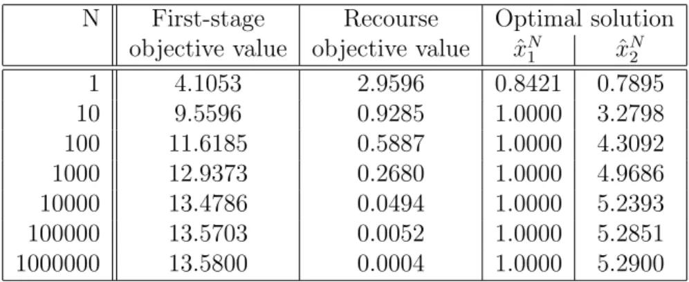
Table 1: Optimal values and solutions for simple recourse model.
N First-stage Recourse Optimal solution objective value objective value xˆN1 xˆN2
1 4.1053 2.9596 0.8421 0.7895
10 9.5596 0.9285 1.0000 3.2798
100 11.6185 0.5887 1.0000 4.3092
1000 12.9373 0.2680 1.0000 4.9686
10000 13.4786 0.0494 1.0000 5.2393
100000 13.5703 0.0052 1.0000 5.2851
1000000 13.5800 0.0004 1.0000 5.2900
Table 2: Optimal values and solutions for probabilistic program.
ε Objective Optimal solution value xˆε1 xˆε2 0,2 9.4438 1.0000 3.2219 0,1 10.2349 1.0000 3.6174 0,05 10.8899 1.0000 3.9450 0,01 12.1382 1.0000 4.5691 0,001 13.5754 1.0000 5.2877
When comparing results from tables 1 and 2, we observe that optimal solu- tions and optimal values of (23) and (24) behave similarly with increasing N and decreasing ε, respectively. A question is if there is a quantitative relation between the outputs of the two models in dependence on the choice of parameters N and ε.
The two problems (21) and (22) are not equivalent. However, by intuition one may expect that for a given ε >0 there exists N large enough such that the obtained optimal solution, say xN(P), of (22) satisfies the probabilistic constraint (5). Then the corresponding value ofEPf(xN(P), ω) may serve as an upper bound for the optimal value of (21). This conjecture is supported by the analysis of optimality conditions for the simple recourse problem with random right-hand sides; they provide a link between the simple-recourse penalty coefficients and the values of the probability thresholds for the corre- sponding problem with individual probabilistic constraints and random right- hand sides, cf. Section 3.2 of [2].
A more complicated form of penalty may be designed as the optimal value of the recourse function q(x, ω) of the second-stage linear program miny{q>y : W y ≥b(ω)−T(ω)x, y ≥ 0} with some q ∈IRm+ and a fixed recourse matrix W; problem (22) corresponds to qk = N∀k and the simple recourse matrix W = I. For a numerical evidence see also [15] where a piecewise linear nonseparable penalty functionN[maxj(xj−ωj)]+was applied and the results compared with those obtained for joint probabilistic constraint of the type P{xj ≤ωj, j = 1, . . . , n} ≥1−ε.
Also convexity preserving penalty functions, say ϑ : IRm → IR+ which are continuous, nondecreasing in their components and are equal to 0 on IRm− and positive otherwise seem to be a suitable choice. This idea stems from the connection between (21) and (22) that can be recognized within the framework ofconvex multiobjective stochastic programming. We shall firstly illustrate it for one of the already considered probabilistic programs. Indeed, the optimal solutions of (21) with Xε(P) given by (5) can be viewed as efficient solutions of the bi-criterial problem
“min”x∈X[F(x, P),−H(x, P)]
obtained by the -constrained approach. Hence, for convex X, F(·, P) = EPf(·, ω) convex and H(·, P) := P(ω : g(·, ω) ≤ 0) concave there exists N ≥ 0 such that these efficient solutions can be found as optimal solutions
of the parametric program
minx∈X[F(x, P)−N ·H(x, P)].
A similar relationship can be established for a whole family of stochastic programs of the form
minx∈X{EPf(x, ω) :EPgk(x, ω)≤k, k = 1, . . . , m} (25) with distribution dependent set of feasible solutions Xε(P). Evidently, pro- blems with probabilistic constraints and those with integrated chance con- straints are special instances of (25). Again, for fixed thresholds k, k = 1, . . . , m, the optimal solutions of (25) may be viewed as efficient solutions of the multiobjective problem
“min”x∈X{EPf(x, ω), EPgk(x, ω), k = 1, . . . , m} (26) obtained by the -constrained approach.
IfX is nonempty, convex, compact and the functionsEPf(x, ω), EPgk(x, ω), k = 1, . . . , m,areconvex inxon IRnthen there exists a nonnegative parame- ter vector t ∈IRm, such that the efficient points can be obtained by solving a scalar convex optimization problem
minx∈X[EPf(x, ω) +
m
X
k=1
tkEPgk(x, ω)]. (27) This scalarization is a special form of scalarization by a penalty function ϑ : IRm →IR which must be continuous and nondecreasing in its arguments to provide efficient solutions of (26):
minx∈X[EPf(x, ω) +N ϑ(EPg1(x, ω), . . . , EPgm(x, ω))] ; (28) N > 0 is a parameter. (For relevant results on multiobjective optimization see e.g. [20].)
A rigorous proof of the relationship between optimal values and solutions of (21) and those of (22) for the penalty function NPmk=1[gk(x, ω)]+ is due to Ermoliev, et. al. [17]. It is valid under modest assumptions on the nonlinear functions gk, on continuity of the probability distribution P and on the structure of problem (21).
The approach by [17] can be further extended to a whole class of penalty functionsϑ.For functionsϑ : IRm →IR+which are continuous nondecreasing in their components, equal to 0 on IRm− and positive otherwise, it holds that
P(gk(x, ω)≤0, 1≤k ≤m)≥1−ε ⇐⇒ P(ϑ(g(x, ω))>0)≤ε.
The considered penalty function problem can be formulated as follows ϕN(P) = min
x∈X
hEPf(x, ξ) +N ·EPϑ(g(x, ω))i (29) with N a positive parameter. We denote xN(P) an optimal solution of (29) and xε(P) an optimal solution of (21) with a levelε∈(0,1).
Theorem 1 For a fixed probability distributionP consider the two problems (21) and (29) and assume: X 6=∅ compact, F(x, P) =EPf(x, ω)a continu- ous function of x,
ϑ : IRm →IR+a continuous function, nondecreasing in its components, which is equal to 0 on IRm− and positive otherwise,
(i) gk(·, ω)∀k are almost surely continuous;
(ii) there exists a nonnegative random variable C(ω)with EPC1+κ(ω)<∞ for some κ >0, such that |ϑ(g(x, ω))| ≤C(ω);
(iii) EPϑ(g(x0, ω)) = 0, for some x0 ∈ X; (iv) P(gk(x, ω) = 0) = 0,∀k, for all x∈ X.
Denote γ =κ/2(1 +κ), and for arbitrary N >0 and ε∈(0,1) put ε(N) = P(ϑ(g(xN(P), ω))>0),
α(N) = N ·EPϑ(g(xN(P), ω)), β(ε) = ε−γEPϑ(g(xε(P), ω)).
THEN for any prescribed ε ∈ (0,1) there always exists N large enough so that minimization (29) generates optimal solutions xN(P) which also satisfy the probabilistic constraints (5) with the given ε.
Moreover, bounds on the optimal value ψε(P) of (21) based on the optimal value ϕN(P) of (29) and vice versa can be constructed:
ϕ1/εγ(N)(P)−β(ε(N)) ≤ ψε(N)(P) ≤ ϕN(P)−α(N),
ψε(N)(P) +α(N) ≤ ϕN(P) ≤ ψ1/N1/γ(P) +β(1/N1/γ), (30) with
N→+∞lim α(N) = lim
N→+∞ε(N) = lim
ε→0+
β(ε) = 0.
Proof:
To simplify the notation for purposes of the proof, we shall drop the argument P used to indicate the dependence of optimal solutions on the probability distribution.
We denote
δN =EPϑ(g(xN, ω))
and assume that for some sequence xN of optimal solutions of the pro- blem (29) δN →0+. Our assumptions and general properties of the penalty function method, see [1, Theorem 9.2.2], ensure existence of such sequence of optimal solutions and also convergence of α(N) =N δN → 0 forN → ∞.
By Chebyshev inequality Pϑ(g(xN, ω))>0=
= P0< ϑ(g(xN, ω))≤qδN+Pϑ(g(xN, ω))>qδN
≤ Gϑ(xN,
q
δN)−Gϑ(xN,0) + 1
√δN
EPϑ(g(xN, ω))
≤ Gϑ(xN,qδN)−Gϑ(xN,0) +qδN →0 as N → ∞.
Here for a fixed x, Gϑ(x,·) denotes the distribution function of ϑ(g(x, ω)) defined by
Gϑ(x, y) =Pϑ(g(x, ω))≤y.
Assumption (iii) implies that for every ε > 0 there exists somexε ∈X such that
P(gk(xε, ω)≤0, 1≤k≤m)≥1−ε.
Then for any ε >0 the following relations hold EPϑ(g(xε, ω)) =
≤
Z
Ω
C(ω)I(ϑ(g(xε,ω))>0)P(dω)
≤
Z
Ω
C1+κ(ω)P(dω)
!1/(1+κ)
·
Z
Ω
I(ϑ(g(xε,ω))>0)P(dω)
!κ/(1+κ)
≤ c·Pϑ(g(xε, ω))>0κ/(1+κ)
≤ c·εκ/(1+κ),
where c:=RΩC1+κ(ω)P(dω)1/(1+κ), which is finite due to the assumption (ii). Accordingly, for ε→0+
0≤EPϑ(g(xε, ω))≤c·εκ/(1+κ) →0.
If we set
ε(N) = Pϑ(g(xN, ω))>0,
then the optimal solutionxN of the expected value problem is feasible for the probabilistic program with ε=ε(N), because the following relations hold
P(gk(xN, ω)≤0, 1≤k≤n)≥1−ε(N)
⇐⇒Pϑ(g(xN, ω))>0≤ε(N).
Hence, we get
ϕN(P) = F(xN, P) +N ·EPϑ(g(xN, ω))
≥ F(xε(N), P) +N ·EPϑ(g(xN, ω))
= ψε(N)(P) +α(N).
Finally,
ψε(P) =
ψε(P) +ε−γEPϑ(g(xε, ω))
−ε−γEPϑ(g(xε, ω))
≥ ϕε−γ(P)−ε−γEPϑ(g(xε, ω))
= ϕε−γ(P)−β(ε).
This completes the proof.
It means that under assumptions of the Theorem, the two problems (21), (29) are asymptotically equivalent which is a useful theoretical result. No- tice, however, that when we want to evaluate one of the bounds in (30), we must be prepared to face some problems. We solve the penalty function problem (29) taking a sufficiently large N > 0 to get its optimal solution xN(P) and optimal value ϕN(P). Then we are able to computeα(N),ε(N), hence the upper bound for the optimal value ψε(N)(P) of the probabilistic program (5) with probability level ε(N). But we are not able to compute β(ε(N)) without having the solution xε(N)(P) which we do not want to find or even may not able to find. We can only solve the penalty function pro- blem with N = 1/εγ(N) getting its optimal solutionx1/εγ(N)(P) and optimal value ϕ1/εγ(N)(P) which is only a part of the lower bound for the optimal value ψε(N)(P).
The bounds (30) and the termsα(N), ε(N) andβ(ε) depend on the choice of the penalty function ϑ. Two special penalty functions are readily available:
ϑ1(u) = Pmk=1[uk]+ applied in [17] and ϑ2(u) = max1≤k≤m[uk]+. However, only ϑ1 preserves convexity, whereas ϑ2 may work better for joint probabi- listic constraints.
The obtained problems with penalties and with a fixed set of feasible soluti- ons are much simpler to solve and analyze then the probabilistic programs;
namely, contamination technique can be used for output analysis of (29) pro- vided that the expectation-type objective function is convex or continuous in x. A question for future research is how to choose the parameter N so that the probability level ε is ensured.
4 Approximate contamination bounds
As discussed in Section 2, to construct global bounds for the optimal value of stochastic programs under contamination of the probability distribution, i.e. with respect to the contamination parameter λ, we need that the op- timal value function ϕ(λ) is concave to get the lower bound in (12). To prove the existence and the form of the directional derivative in the upper bound of (12) one needs further results onstability of the initial program and differentiability of the contaminated objective function.
With the set of feasible solutions dependent on P, concavity of the optimal value function ϕP Q(λ) cannot be guaranteed. Such problems may be ap-
proximated by penalty-type problems which possess a fixed set of feasible first-stage solutions. This in turn opens the possibility to construct approxi- mate contamination bounds.
EXAMPLE 2.
For the general probabilistic program (21), let us accept the problem minx∈X
"
EPf(x, ω) +
m
X
k=1
tkEP[gk(x, ω)]+
#
(31) with convex compact X 6=∅, convex functionsf(·, ω), gk(·, ω), k = 1, . . . , m and a fixed nonnegative parameter vectort∈IRm as an acceptable substitute for the probabilistic program (21)
min{EPf(x, ω) : x∈ X ∩ Xε(P)}
with Xε(P) defined by (5). Denote the random objective in (31) as θ(x, ω;t) = f(x, ω) +
m
X
k=1
tk[gk(x, ω)]+. Using this notation, we rewrite (31) as
minx∈X Θ(x, P;t) :=EPθ(x, ω;t).
The set of feasible solutions X does not depend on P and for fixed vectors t, the contamination bounds for the optimal value ϕt(Pλ) of (31) for con- taminated probability distribution (10) follow the usual pattern (13). They may serve as an indicator of robustness of the optimal value of (21) and may support decisions about the choice of weights tk.
EXAMPLE 3.
In the model of [3], the second-stage variables yare supposed to satisfy with a prescribed probability 1−δ certain constraints driven by another random factor, η, whose probability distribution is independent ofP.The problem is
minx∈XF(x, P, S) :=EPf(x, ω, S) =c>x+
Z
Ω
R(x, ω, S)P(dω) (32) where
R(x, ω, S) = min
y {q>y :W y =h(ω)−T(ω)x, y ∈IRr+, S(Ay≤η)≥1−δ}, (33)
S denotes the probability distribution of s-dimensional random vectorη and A(s, r) is a deterministic matrix composed of rows Aj, j = 1, . . . , s. With respect to P, (32) is an expectation type of stochastic program, with a fi- xed set X of feasible first-stage decisions and with an incomplete recourse;
hence, there is a good chance to construct contamination bounds on the op- timal valueϕ(Pλ, S) of (32) for afixed probability distribution S and for the contaminated probability distribution Pλ.
Assume thatT is nonrandom with a full row rank,Sis fixed and such that the set YS := ny∈IRr+ : S(Ay ≤η)≥1−δo is convex and bounded. Let the set X∗(P, S) of optimal solutions of (32) be nonempty and bounded. Under further assumptions which guarantee finiteness and convexity of the second stage value function R(·, ω, S) for a fixed probability distribution S (hence finiteness and convexity of the random objective value function f(·, ω, S)), assumptions on existence of its expectation with respect to P and Q and assumptions on joint continuity of F(·,·, S) in the decision vector x and the probability measureP, cf. [3], the directional derivative of the optimal value function ϕ(·, S) at P in the direction Q−P exists and is of the form (11), i.e.
x∈Xmin∗(P,S)F(x, Q, S)−ϕ(P, S). (34) Similar contamination bounds on the optimal value function can be deri- ved even without assumptions which guarantee that the random objective function is convex in x. To this purpose, general contamination results of [9]
and stability results of [3] may be exploited; cf. [4]. It is important, however, that some continuity properties hold true. This simplifies in case that the probability distribution P is absolutely continuous.
IfS is a discrete probability distribution then for a fixedxandω the penalty R(x, ω, S) can be evaluated by the approach of [29]. To solve the mixed program (32) and to construct contamination bounds based on (34) it would be necessary to modify the algorithm to the case of parametrized right-hand sides h(ω)−T xof the second-stage problem (33).
To model perturbations with respect toSand to construct the corresponding contamination bounds is more demanding. A possibility is to replace the probabilistic constraint in (33) by an expected (with respect to S) penalty term added to q>y, as done e.g. in (22):
R(x, ω, S)≈
miny {q>y+N
s
X
j=1
ES[Ajy−ηj]+ : W y=h(ω)−T(ω)x, y ≥0}:= ˜R(x, ω, S).
The approximate problem minx∈X
F˜(x, P, S) :=EPf˜(x, ω, S) =c>x+
Z
Ω
R(x, ω, S˜ )P(dω)
is linear in P and concave in S, X is independent of P, S which allows to construct contamination bounds for contaminated probability distributionS, too. In this case, however, existence of the directional derivative (15) must be examined in detail.
5 Conclusions
Contamination technique is known to be a suitable tool to robustness analy- sis of penalty-type stochastic programs with respect to changes of probability distributions. It provides global bounds for the optimal value of stochastic program with respect to perturbations of the probability distribution mo- deled via contamination. As the set of feasible decisions of probabilistic programs depends on the probability distribution, the possibility of obtai- ning similar global results for probabilistic programs is limited to problems of a very special form and/or under special distributional assumptions; see Examples 1 and 3 for an illustration and discussion.
Reformulation of probabilistic programs by incorporating a suitably chosen penalty function into the objective helps to arrive at problems with a fixed set of feasible solutions which in turn opens the possibility of construction of the convexity-based contamination bounds. The recommended form of the penalty function follows the basic ideas of multiobjective programming and its suitable properties follow by generalization of results of [17].
For expectation-type objectives, conditions for differentiability with respect to the contamination parameter of the contaminated objective function re- duce mostly to continuity or convexity of the two noncontaminated objecti- ves. For general types of objectives, to derive the existence and the form of these directional derivatives the local qualitative stability results play an important role.
Acknowledgements. This research is supported by the project “Methods of modern mathematics and their applications” – MSM 0021620839 and by the Grant Agency of the Czech Republic (grants 402/08/0107 and 201/05/H007).
References
[1] Bazaraa, M. S., Sherali, H. D., Shetty, C. M. (1993),Nonlinear Programming:
Theory and Algorithms, Wiley, Singapore.
[2] Birge, J. R., Louveaux, F. (1997), Introduction to Stochastic Programming, Springer Series on Oper. Res., New York.
[3] Bosch, P., Jofr´e, A., Schultz, R. (2007), Two-stage stochastic programs with mixed probabilities, SIAM. J. Optim. 18, 778–788.
[4] Branda, M. (2008), Local stability and differentiability of mixed stochastic programming problems, WP, KPMS MFF UK, Prague.
[5] Danskin, J. M. (1967), Theory of Max-Min, Springer, Berlin (Econometrics and Operations Research 5).
[6] Dobi´aˇs, P. (2003), Contamination for stochastic integer programs,Bull. Czech Econometric Soc.18, 65–80.
[7] Dupaˇcov´a, J. (1986), Stability in stochastic programming with recourse – contaminated distributions, Math. Programming Study 27, 133–144.
[8] Dupaˇcov´a, J. (1987), Stochastic programming with incomplete information:
A survey of results on postoptimization and sensitivity analysis,Optimization 18, 507–532.
[9] Dupaˇcov´a, J. (1990), Stability and sensitivity analysis in stochastic progra- mming,Ann. Oper. Res. 27, 115-142.
[10] Dupaˇcov´a, J. (1996), Scenario based stochastic programs: Resistance with respect to sample, Ann. Oper. Res.64, 21–38.
[11] Dupaˇcov´a, J. (2006), Contamination for multistage stochastic programs.
In: Huˇskov´a, M., Janˇzura, M. (eds.) Prague Stochastics 2006, Matfyzpress, Praha, pp. 91–101.
[12] Dupaˇcov´a, J. (2006), Stress testing via contamination. In: Marti, K. et al.
(eds.), Coping with Uncertainty, Modeling and Policy Issues, LNEMS 581, Springer, Berlin, pp.29–46.
[13] Dupaˇcov´a, J. (2008) Risk objectives in two-stage stochastic programming problems, Kybernetika44, 227–242.
[14] Dupaˇcov´a, J., Bertocchi, M. and Moriggia, V. (1998), Postoptimality for scenario based financial models with an application to bond portfolio ma- nagement. In: Ziemba, W. T. and Mulvey, J. (eds.) World Wide Asset and Liability Modeling. Cambridge Univ. Press, 1998, pp. 263–285.
[15] Dupaˇcov´a, J., Gaivoronski, A. A., Kos, Z., Sz´antai, T. (1991), Stochastic pro- gramming in water management: A case study and a comparison of solution techniques, European J. Oper. Res. 52, 28–44.
[16] Dupaˇcov´a, J., Pol´ıvka, J. (2007), Stress testing for VaR and CVaR, Quanti- tiative Finance 7, 411–421.
[17] Ermoliev, Y. M., Ermolieva, T., MacDonald, G. J., Norkin, V. I. (2000), Stochastic optimization of insurance portfolios for managing expose to cata- strophic risks, Ann. Oper. Res.99, 207–225.
[18] Fiacco, A. V. (1983), Introduction to Sensitivity and Stability Analysis in Nonlinear Programming. Academic Press, New York.
[19] Gol’ˇstejn, E. G. (1972), Theory of Convex Programming, Translations of Mathematical Monographs 36, American Mathematical Society, Providence, RI.
[20] Guddat, J., Guerra Vasquez, F., Tammer, K., Wendler, K. (1985), Multi- objective and Stochastic Optimization Based on Parametric Optimization, Akademie-Verlag, Berlin.
[21] Kall, P. (1987), On approximations and stability in stochastic programming.
In: Guddat, J. et al. (eds.) Parametric Optimization and Related Topics.
Akademie-Verlag, Berlin, pp. 387–400.
[22] Kall, P., Mayer, J. (2005), Stochastic Linear Programming: Models, Theory and Computation. Springer International Series, New York.
[23] Kall, P., Mayer, J. (2005), Building and solving stochastic linear programming models with SLP-IOR. In: Wallace, S.W., Ziemba, W.T. (eds.),Applications of stochastic programming, MPS-SIAM Book Series on Optimization 5.
[24] Kall, P., Ruszczy´nski, A., Frauendorfer, K. (1988), Approximation techniques in stochastic programming. In: Ermoliev, Yu., Wets, R. J-B. (eds.),Numerical Techniques for Stochastic Optimization, Springer, Berlin, pp.34–64.
[25] Kan, Y. S., Kibzun, A. I. (2000), Sensitivity analysis of worst-case distribution for probability optimization problems. In: Uryasev, S.P. (ed.), Probabilistic Constrained Optimization, Kluwer Acad. Publ., pp. 132–147.
[26] Klein Haneveld, W. K. (1986), Duality in Stochastic Linear and Dynamic Programming, LNEMS274, Springer, Berlin.
[27] Pr´ekopa, A. (1971), Logarithmic concave measures with application to sto- chastic programming, Acta Sci. Math. (Szeged) 32, 301–316.
[28] Pr´ekopa, A. (1973), Contributions to the theory of stochastic programming, Math. Program. 4, 202–221.
[29] Pr´ekopa, A. (2007), On the relationship between probabilistic constrained, disjunctive and multiobjective programming, RRR 7–2007, Rutcor, Rutgers University, New Jersey.
[30] R¨omisch, W. (2003), Stability of stochastic programming problems. Chapter 8 in: [31], pp. 483–554.
[31] Ruszczynski, A., Shapiro A. (eds.) (2003), Handbook on Stochastic Program- ming, Elsevier, Amsterdam.
[32] Serfling, R. J. (1980), Approximation Theorems of Mathematical Statistics, Wiley, New York.
[33] Shapiro, A. (1990), On differential stability in stochastic programming,Math.
Program. 47, 107–116.