Rising Mediterranean Sea Surface Temperatures Amplify
1
Extreme Summer Precipitation in Central Europe
2
SUPPLEMENTARY INFORMATION
3
Claudia Volosciuk*1, Douglas Maraun1,2, Vladimir A. Semenov1,3,4, Natalia Tilinina5, Sergey K.
4
Gulev5 & Mojib Latif1
5
Content
6
• Evaluation of Model Experiments
7
• Table S1
8
• Figures S1–S11; in all Figures:
9
– Heavy precipitation events are days on which daily precipitation aggregated over
10
15 – 22◦E, 46 – 51◦N (red box in Fig. 2 in the main paper) exceeds the 95th percentile
11
of all summer days in the respective model experiment.
12
– Significance is tested based on a two-sided independent samples t-test. Differences
13
between composites on heavy precipitation events (summer mean climatologies) are
14
tested at the 90% (95%) significance level.
15
Evaluation of Model Experiments
16
Summer mean precipitation in our ECHAM5 model experiments (Fig. S1a, b) is evaluated
17
with the European daily high-resolution (0.25◦ × 0.25◦) gridded dataset (E-OBS, version 10) of
18
precipitation1 (Fig. S1c), developed in the framework of the ENSEMBLES project. E-OBS at
19
0.25◦ was averaged to the resolution of the model simulations by area conservative remapping.
20
As summer mean precipitation climatologies in our sensitivity experiments (Fig. S1a, b) are very
21
similar (Fig. S1d) we compare both experiments to the E-OBS precipitation climatology over both
22
forcing periods, i.e., 1970 – 2012 (Fig. S1c). The precipitation pattern over Europe is well captured
23
in both experiments. Major deficiencies are a wet bias at the Scandinavian west coast and a dry
24
bias in eastern Austria. Central and Eastern Europe are slightly wetter in the experiments than in
25
the observations. These differences are small, and the overall pattern is well captured. The bias is
26
very low for both experiments (Tab. S1).
27
We did not evaluate simulated 20-summer return levels with the E-OBS dataset as the rain
28
gauge density in E-OBS is sparse in some regions, especially in Eastern Europe1. Hence, extreme
29
precipitation is likely to be underrepresented in these regions by the E-OBS dataset, and differences
30
between the model simulations and observations are therefore not necessarily attributable to model
31
deficiencies.
32
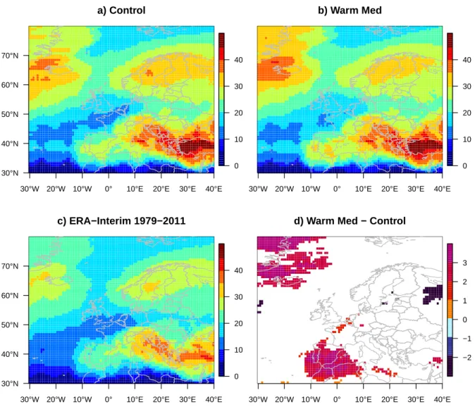
Summer mean cyclone track densities in our experiments (Fig. S2a, b) are evaluated with
33
ERA-Interim reanalysis2, 3 (Fig. S2c). The summer cyclone track pattern is well captured over
34
Interim. This has already been reported for ECHAM5 simulations compared with ERA404. Al-
36
though ECHAM5 generally simulates more cyclones Nissen et al., 20134 found the share of
37
Mediterranean cyclones developing into Vb-cyclones to be similar in coupled ECHAM5 scenario
38
simulations and ERA40. In our experiments, the Mediterranean storm track is also stronger than
39
in reanalysis (ERA-Interim in our case) with the strongest bias located over Turkey. The bias of
40
the European mean is∼4 cyclones per summer in both experiments (Tab. S1).
41
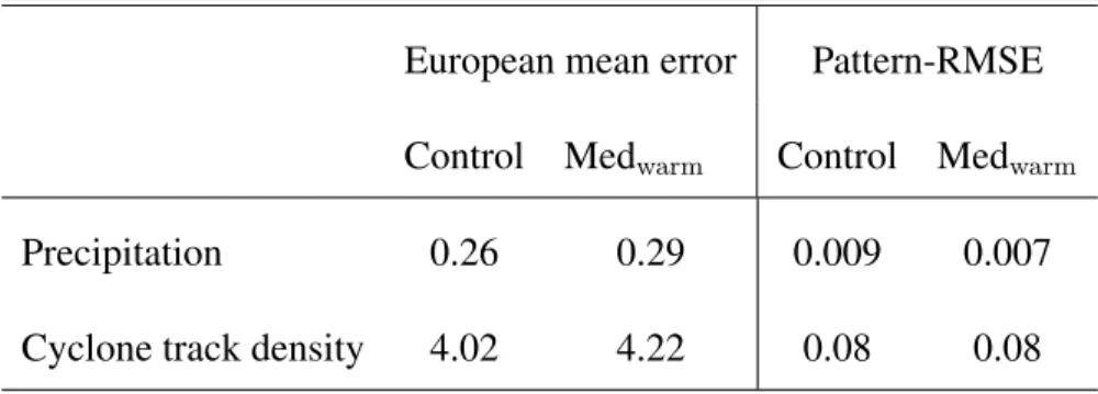
Table S1: Bias of summer mean precipitation and cyclone tracks in model experiments.Error of simulated European mean (10◦W–40◦E, 30–70◦N) and root mean squared error (RMSE) of the pattern for JJA mean precipitation (mm/day) and JJA mean cyclone track density (cyclones per summer) in the ECHAM5 control and Medwarm experiments evaluated against the E-OBS precipitation gridded dataset and cyclone tracks from ERA-Interim reanalysis
European mean error Pattern-RMSE Control Medwarm Control Medwarm
Precipitation 0.26 0.29 0.009 0.007
Cyclone track density 4.02 4.22 0.08 0.08
42 1. Haylock, M. R.et al. A European daily high-resolution gridded data set of surface temperature
43
and precipitation for 1950–2006. Journal of Geophysical Research113, D20119 (2008).
44
2. Dee, D. P.et al. The ERA-Interim reanalysis: configuration and performance of the data assim-
45
ilation system. Quarterly Journal of the Royal Meteorological Society137, 553–597 (2011).
46
3. Tilinina, N., Gulev, S. K., Rudeva, I. & Koltermann, P. Comparing cyclone life cycle character-
47
istics and their interannual variability in different reanalyses. Journal of Climate26, 6419–6438
48
(2013).
49
4. Nissen, K. M., Ulbrich, U. & Leckebusch, G. C. Vb cyclones and associated rainfall ex-
50
tremes over Central Europe under present day and climate change conditions. Meteorologische
51
Zeitschrift 22, 649–660 (2013).
52
0 1 2 3 4 5
a) Control
10°W 0° 10°E 20°E 30°E 40°E
30°N 40°N 50°N 60°N 70°N
0 1 2 3 4 5
b) Warm Med
10°W 0° 10°E 20°E 30°E 40°E
0 1 2 3 4 5
c) E−OBS 1970−2012
10°W 0° 10°E 20°E 30°E 40°E
30°N 40°N 50°N 60°N 70°N
−0.4
−0.2 0.0 0.2 0.4 0.6
10°W 0° 10°E 20°E 30°E 40°E
d) Warm Med − Control
Figure S1: Summer mean precipitation. Mean JJA precipitation (mm/day) in (a) control experi- ment, (b) warm Mediterranean (Medwarm) experiment, and (c) E-OBS, version 10. (d) Significant differences between JJA-climatology in Medwarm and control. Maps created with R version 3.2.3 (www.r-project.org).
0 10 20 30 40
30°W 20°W 10°W 0° 10°E 20°E 30°E 40°E 30°N
40°N 50°N 60°N 70°N
a) Control
0 10 20 30 40
30°W 20°W 10°W 0° 10°E 20°E 30°E 40°E
b) Warm Med
0 10 20 30 40
30°W 20°W 10°W 0° 10°E 20°E 30°E 40°E 30°N
40°N 50°N 60°N 70°N
c) ERA−Interim 1979−2011
−2
−1 0 1 2 3
30°W 20°W 10°W 0° 10°E 20°E 30°E 40°E
d) Warm Med − Control
Figure S2: Summer cyclone track densities. Mean JJA cyclone track densities (cyclones per summer) in (a) control experiment, (b) Medwarm experiment, and (c) ERA-Interim. Counts of cyclone centres that pass within 500 km of a grid point. (d) Significant differences between JJA- climatology in Medwarmand control. Maps created with R version 3.2.3 (www.r-project.org).
0 3 6 9 12 15 18 21 [mm d−1]
a) Control
10°W 0° 10°E 20°E 30°E 40°E 30°N
40°N 50°N 60°N 70°N
0 3 6 9 12 15 18 21
[mm d−1]
b) Warm Med
10°W 0° 10°E 20°E 30°E 40°E
0 3 6 9 12 15 18 21
[mm d−1]
c) Global warm
10°W 0° 10°E 20°E 30°E 40°E
0 3 6 9 12 15 18 25
[mm d−1]
10°W 0° 10°E 20°E 30°E 40°E 30°N
40°N 50°N 60°N 70°N
d) Elbe flood 2002
0 3 6 9 12 15 18 32
[mm d−1]
10°W 0° 10°E 20°E 30°E 40°E
e) Oder flood 2010
0 3 6 9 12 15 18 58
[mm d−1]
10°W 0° 10°E 20°E 30°E 40°E
f) Danube flood 2013
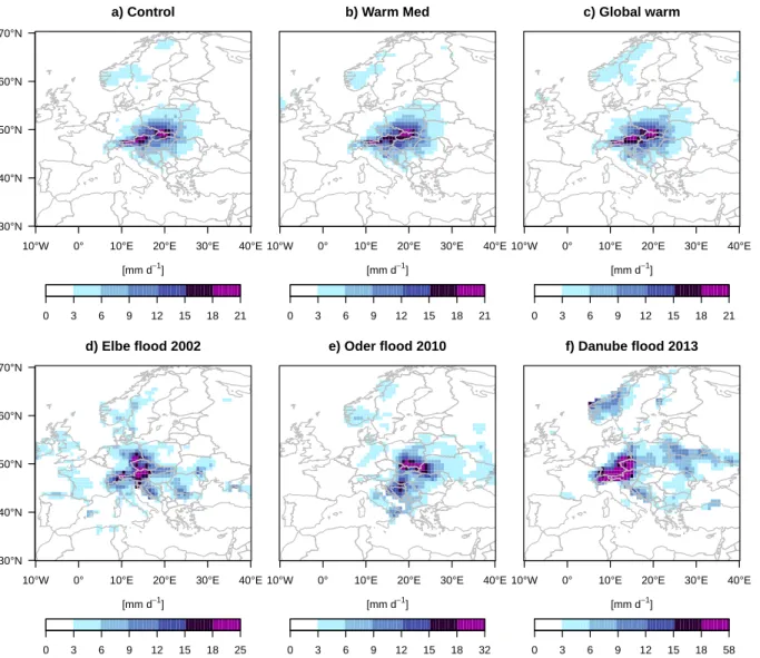
Figure S3:Precipitation on heavy-precipitation events. (a – c) Composites of daily precipitation on heavy-precipitation events in model experiments. In all experiments precipitation maxima on heavy-precipitation events are in Austria and Slovakia. (a) Control, (b) Medwarm, and (c) Globwarm. (d – f) Observed (E-OBS, version 10) aggregated precipitation on recent heavy-precipitation events caused by Vb-cyclones that led to severe flooding, normalised by the number of event days. (d) Elbe 2002, (e) Oder 2010, and (f) Danube 2013. Note the different colour scales. Composites (a – c) represent an average of several events where single peaks are smoothed, and can thus not directly be compared to single cases (d – f). Nevertheless, the affected regions by the three cases are similar to the composites of our model experiments. Note that the study region for the heavy events in the composites constrains the affected region. Maps created with R version 3.2.3 (www.r-project.org).
5°E 10°E 15°E 20°E 25°E 42°N
46°N 50°N 54°N
a) MAM
−40
−20 0 20 40 [%]
5°E 10°E 15°E 20°E 25°E
42°N 46°N 50°N 54°N
b) SON
Figure S4:Changes in 20-season return levels.Medwarmcompared to control. (a) Spring (March- April, MAM), and (b) autumn (September-November, SON). Maps created with R version 3.2.3 (www.r-project.org).
10°W 0° 10°E 20°E 30°E 40°E 30°N
40°N 50°N 60°N 70°N
Figure S5: Identification of Vb-cyclones. Cyclone tracks are identified as Vb-cyclones if they fulfill the following criteria: (1) cyclone must pass the typical Vb-cyclogenesis area (5 – 15◦E &
40 – 45◦N, red box), (2) cyclone must cross 47◦N (horizontal blue line) between 10–25◦E (vertical blue lines). Map created with R version 3.2.3 (www.r-project.org).
−6 −4 −2 0 1 2 [hPa]
10°W 0° 10°E 20°E 30°E 40°E 30°N
40°N 50°N 60°N 70°N
a) CTL
−6 −4 −2 0 1 2
[hPa]
10°W 0° 10°E 20°E 30°E 40°E
b) CTL; Lag 1 anom.
−6 −4 −2 0 1 2
[hPa]
10°W 0° 10°E 20°E 30°E 40°E
c) CTL, Lag 2 anom.
1005 1009 1013 1017 [hPa]
10°W 0° 10°E 20°E 30°E 40°E 30°N
40°N 50°N 60°N 70°N
d) CTL; clim.
0 0.5 1 1.5
[hPa]
10°W 0° 10°E 20°E 30°E 40°E
e) Warm Med − CTL; clim.
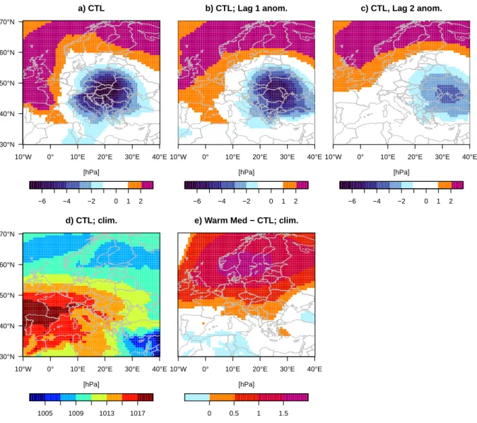
Figure S6: Sea level pressure. (a – c) Composites of mean sea level pressure (hPa) anomalies (relative to climatology) in the control experiment on heavy-precipitation events and on the two preceding days. No significant differences between composites from the Medwarm and control experiments were found. (d) JJA-climatology in the control experiment. (e) Significant differences between JJA-climatology in Medwarm and control. Maps created with R version 3.2.3 (www.r- project.org).
0 2 4 6 8 10 12
10°W 0° 10°E 20°E 30°E 40°E 30°N
40°N 50°N 60°N 70°N
a) Control
0 1 2 3 4
10°W 0° 10°E 20°E 30°E 40°E b) Warm Med − Control
−12 −10 −8 −6 −4 −2 0
0.000.050.100.150.20
c) Max. deepening rate
Max. deepening rate [hPa/6hrs]
Density
Control Warm Med
960 980 1000 1020 1040
0.000.010.020.03
d) Min. core SLP
Min. core SLP [hPa]
Density
Control Warm Med
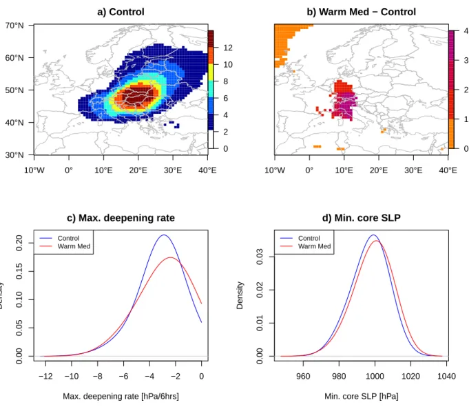
Figure S7: Reduced dynamics of heavy-precipitation causing cyclones.Cyclone tracks passing over 15 – 22◦E, 46 – 51◦N (red box in Fig. 2 in the main paper) on heavy-precipitation events are considered. (a) Summer (JJA) cyclone frequency in control experiment. Counts of cyclone centres that pass within 500 km of a grid point. Unit: 6-hourly time steps per summer. (b) Significant differences between cyclone frequency in Medwarm and control, indicating slower travelling cy- clones in Medwarmexperiment. (c) Density of cyclone-centre maximum deepening rate (hPa/6hrs), indicating slower deepening of cyclones in Medwarm experiment. (d) Density of minimum core pressure (hPa), indicating slightly less deep cyclones in Medwarm experiment. Maps created with R version 3.2.3 (www.r-project.org).
−3 −1 0 1 2 3 4 5 [kg m−2]
10°W 0° 10°E 20°E 30°E 40°E 30°N
40°N 50°N 60°N 70°N
a) CTL; Lag 1 anom.
−3 −1 0 1 2 3 4 5
[kg m−2]
10°W 0° 10°E 20°E 30°E 40°E
b) CTL; Lag 2 anom.
10 15 20 25 30
[kg m−2]
10°W 0° 10°E 20°E 30°E 40°E
c) CTL; clim.
−1 −0.5 0 0.5 1 1.5 [kg m−2]
10°W 0° 10°E 20°E 30°E 40°E 30°N
40°N 50°N 60°N 70°N
d) Warm Med − CTL; Lag 1
−1 −0.5 0 0.5 1 1.5 [kg m−2]
10°W 0° 10°E 20°E 30°E 40°E
e) Warm Med − CTL; Lag 2
−0.5 0 0.5 1 1.5
[kg m−2]
10°W 0° 10°E 20°E 30°E 40°E
f) Warm Med − CTL; clim.
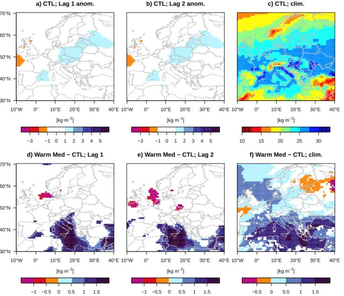
Figure S8: Precipitable water. Composites of column integrated precipitable water (kg m−2) on (a, d) lag 1 and (b, e) lag 2 days before heavy-precipitation events: (a, b) anomalies in control ex- periment (relative to climatology) and (d, e) significant differences between composites in Medwarm
and control. (c) JJA-climatology of control experiment. (f) Significant differences between JJA- climatology in Medwarmand control. Maps created with R version 3.2.3 (www.r-project.org).
−25 −15 −5 5 15 25 [10−5 kg m−2s−1]
10°W 0° 10°E 20°E 30°E 40°E 30°N
40°N 50°N 60°N 70°N
a) CTL; Lag 1 anom.
−25 −15 −5 5 15 25
[10−5 kg m−2s−1]
10°W 0° 10°E 20°E 30°E 40°E
b) CTL; Lag 2 anom.
−25 −15 −5 5 15 25
[10−5 kg m−2s−1]
10°W 0° 10°E 20°E 30°E 40°E
c) CTL; clim.
−5 −3 −1 1 3 5
[10−5 kg m−2s−1]
10°W 0° 10°E 20°E 30°E 40°E 30°N
40°N 50°N 60°N 70°N
d) Warm Med − CTL; Lag 1
−5 −3 −1 1 3 5
[10−5 kg m−2s−1]
10°W 0° 10°E 20°E 30°E 40°E
e) Warm Med − CTL; Lag 2
−3 −2 −1 0 1 2 3
[10−5 kg m−2s−1]
10°W 0° 10°E 20°E 30°E 40°E
f) Warm Med − CTL; clim.
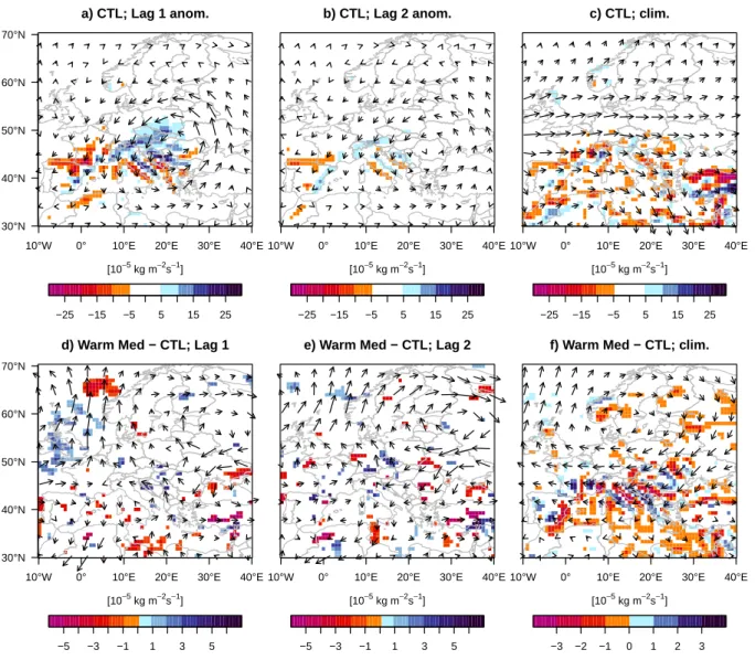
Figure S9: Moisture convergence and moisture transport. Same as Fig. S8 but for vertically integrated moisture convergence (10−5 kg m−2s−1) and vertically integrated moisture transport as vectors (every fifth vector is plotted), vector length is (a - c) 50 kg m−1s−1 per degree lon/lat and (d - f) 10 kg m−1s−1 per degree lon/lat. Maps created with R version 3.2.3 (www.r-project.org).
−1 0 1 2 3 4 [mm d−1]
10°W 0° 10°E 20°E 30°E 40°E 30°N
40°N 50°N 60°N 70°N
a) CTL; Lag 1 anom.
−1 0 1 2 3 4
[mm d−1]
10°W 0° 10°E 20°E 30°E 40°E
b) CTL; Lag 2 anom.
0 0.5 1 1.5 2 2.5 3 3.5 [mm d−1]
10°W 0° 10°E 20°E 30°E 40°E
c) CTL; clim.
0 0.5 1 1.5
[mm d−1]
10°W 0° 10°E 20°E 30°E 40°E 30°N
40°N 50°N 60°N 70°N
d) Warm Med − CTL; Lag 1
0 0.5 1 1.5
[mm d−1]
10°W 0° 10°E 20°E 30°E 40°E
e) Warm Med − CTL; Lag 2
−0.2 0 0.2 0.4 0.6 0.8 [mm d−1]
10°W 0° 10°E 20°E 30°E 40°E
f) Warm Med − CTL; clim.
Figure S10: Evaporation. Same as Fig. S8 but for evaporation (mm d−1). Maps created with R version 3.2.3 (www.r-project.org).
10°W 0° 10°E 20°E 30°E 40°E 30°N
40°N 50°N 60°N 70°N
a) Composite
−5
−3 0 3 5 7 9
[%]
10°W 0° 10°E 20°E 30°E 40°E 30°N
40°N 50°N 60°N 70°N
b) JJA Clim.
Figure S11: Specific humidity increase beyond Clausius-Clapeyron rate. Difference (%) be- tween vertically integrated (up to 200 hPa) specific humidity in Medwarm experiment and the Clausius-Clapeyron related amplification (7% per degree of warming) of the same quantity in the control, based on the temperature difference between Medwarm and control. 0% would be the specific humidity increase based on Clausius-Clapeyron. (a) Composite of heavy-precipitation events, and (b) climatological summer (JJA) mean average. Maps created with R version 3.2.3 (www.r-project.org).