Radium-228-derived ocean mixing and trace element inputs in the South Atlantic

(1)

https://doi.org/10.5194/bg-18-1645-2021

Radium-228-derived ocean mixing and trace element inputs in the South Atlantic

Yu-Te Hsieh¹, Walter Geibert², E. Malcolm S. Woodward³, Neil J. Wyatt⁴, Maeve C. Lohan⁴, Eric P. Achterberg^4,5, and Gideon M. Henderson¹

1Department of Earth Sciences, University of Oxford, Oxford, UK

2Alfred Wegener Institute Helmholtz Centre for Polar and Marine Research, Bremerhaven, Germany

3Plymouth Marine Laboratory, Plymouth, UK

4Ocean and Earth Sciences, National Oceanography Centre, Southampton, UK

5GEOMAR Helmholtz Centre for Ocean Research, Kiel, Germany Correspondence:Yu-Te Hsieh (yu-te.hsieh@earth.ox.ac.uk) Received: 9 October 2020 – Discussion started: 13 October 2020

Revised: 20 January 2021 – Accepted: 8 February 2021 – Published: 9 March 2021

Abstract.Trace elements (TEs) play important roles as micronutrients in modulating marine productivity in the global ocean. The South Atlantic around 40^◦S is a prominent region of high productivity and a transition zone between the nitrate-depleted subtropical gyre and the iron-limited Southern Ocean. However, the sources and fluxes of trace elements to this region remain unclear. In this study, the distribution of the naturally occurring radioisotope ²²⁸Ra in the water column of the South Atlantic (Cape Basin and Argentine Basin) has been investigated along a 40^◦S zonal transect to estimate ocean mixing and trace element supply to the surface ocean. Ra-228 profiles have been used to determine the horizontal and vertical mixing rates in the near-surface open ocean. In the Argentine Basin, horizontal mixing from the continental shelf to the open ocean shows an eddy diffusion ofK_x=1.8±1.4 (10⁶cm²s⁻¹) and an integrated advection velocityw=0.6±0.3 cm s⁻¹. In the Cape Basin, horizontal mixing is K_x=2.7±0.8 (10⁷cm²s⁻¹) and vertical mixingK_z=1.0–1.7 cm²s⁻¹in the upper 600 m layer. Three different approaches (²²⁸Ra diffusion, ²²⁸Ra advection, and ²²⁸Ra/TE ratio) have been applied to estimate the dissolved trace element fluxes from the shelf to the open ocean. These approaches bracket the possible range of off-shelf fluxes from the Argentine Basin margin to be 4–21 (×10³) nmol Co m⁻²d⁻¹, 8–19 (×10⁴) nmol Fe m⁻²d⁻¹ and 2.7–6.3 (×10⁴) nmol Zn m⁻²d⁻¹. Off-shelf fluxes from the Cape Basin margin are 4.3–6.2 (×10³) nmol Co m⁻²d⁻¹, 1.2–3.1 (×10⁴) nmol Fe m⁻²d⁻¹,

and 0.9–1.2 (×10⁴) nmol Zn m⁻²d⁻¹. On average, at 40^◦S in the Atlantic, vertical mixing supplies 0.1–

1.2 nmol Co m⁻²d⁻¹, 6–9 nmol Fe m⁻²d⁻¹, and 5–

7 nmol Zn m⁻²d⁻¹ to the euphotic zone. Compared with atmospheric dust and continental shelf inputs, vertical mixing is a more important source for supplying dissolved trace elements to the surface 40^◦S Atlantic transect. It is insufficient, however, to provide the trace elements removed by biological uptake, particularly for Fe. Other inputs (e.g.

particulate or from winter deep mixing) are required to balance the trace element budgets in this region.

1 Introduction

Trace elements (TEs) play important roles as micronutrients for marine productivity in the surface ocean (Morel and Price, 2003; Lohan and Tagliabue, 2018). For example, iron, zinc, and cobalt are known to be essential micronutrients for the cellular metabolic enzymes in marine phytoplankton, and hence they co-limit primary productivity in some ocean regions. The southern subtropical convergence (SSTC) in the South Atlantic, near 40^◦S (Fig. 1), is a prominent high-productivity region (0.2–

0.3 mg chlorophyllam⁻³; Longhurst, 2007) and a transition zone between the nitrate-depleted subtropical gyre and the iron-limited Southern Ocean, creating one of the most dynamic nutrient environments in the global oceans (Moore et

(2)

al., 2004). However, the trace element sources and fluxes that fuel this region remain poorly constrained. Modelling and experimental studies have both suggested that this region is iron limited or co-limited (Moore et al., 2004; Browning et al., 2014, 2017). It also has the lowest reported dissolved zinc concentrations in the global oceans (Wyatt et al., 2014), and the replacement for zinc by cobalt is crucial for phytoplankton, particularly in low-zinc regions (Price and Morel, 1990).

Thus, knowing the sources and fluxes of iron, zinc, and cobalt can improve our understanding of the limiting factors for productivity in this highly productive region.

Oceanic mixing and advection facilitate the transport of nutrients to the euphotic zone (Oschlies, 2002). The distribution of TEs in the surface ocean is primarily controlled by the inputs from the continental shelves (i.e. rivers, submarine groundwater discharge (SGD), and sediments), deep ocean waters (regeneration, continental slopes, and hydrothermal vents) and aeolian inputs, with these mediated by lateral and vertical mixing (diffusive/turbulent mixing), advection, particle scavenging and biological uptake. In particular, deep winter mixing has been shown to be an important mechanism bringing TEs from below the mixed layer to the surface ocean (Tagliabue et al., 2014; Achterberg et al., 2018, 2020; Rigby et al., 2020). Geochemical tracers for ocean mixing can therefore be used to indirectly estimate TE inputs and outputs in the upper ocean, e.g. tritium (³He) (Jenk- ins, 1988; Schlitzer, 2016) and radium isotopes (²²⁸Ra) (Cai et al., 2002; Ku et al., 1995; Nozaki and Yamamoto, 2001;

Sarmiento et al., 1990; Moore, 2000; Charette et al., 2007;

Sanial et al., 2018).

The four naturally occurring radium isotopes cover a wide range of half-lives (²²⁶Ra,T1/2=1600 years;²²⁸Ra,T1/2= 5.75 years; ²²³Ra, T1/2=11.4 d; ²²⁴Ra, T1/2=3.66 d), which enables us to study oceanic processes at different timescales. Ra-228 is continuously produced through the decay of²³²Th in shelf sediments, released into seawater, and then transported into the surface open ocean by mixing or advection. The half-life of²²⁸Ra is much shorter than the estimated Ra residence time by removal of∼500 years (Moore and Dymond, 1991). The distribution of²²⁸Ra in the ocean is therefore mainly controlled by ocean transport and radioactive decay, and can be used to estimate lateral mixing from the coastal shelf or continental slope to the open ocean (Kauf- man et al., 1973; Knauss et al., 1978; Yamada and Nozaki, 1986; Sanial et al., 2018). Subsequent downward mixing from the surface can also be used to assess vertical mixing in the upper water column (Charette et al., 2007; Sarmiento et al., 1976; van Beek et al., 2008). Radium-228 has also been used as a conservative tracer to estimate submarine groundwater discharge (SGD) (Windom et al., 2006; Moore et al., 2008; Kwon et al., 2014; Rodellas et al., 2015; Le Gland et al., 2017), river inputs (Vieira et al., 2020), continental shelf (Rutgers van der Loeff et al., 1995; Charette et al., 2016; Sa- nial et al., 2018; Kipp et al., 2018a) and hydrothermal inputs (Kipp et al., 2018b).

Previous work has assessed TE inputs to the wider South Atlantic from rivers (Vieira et al., 2020), atmospheric dust (Gaiero et al., 2013), shelf sediments (Graham et al., 2015), the Agulhas current (Paul et al., 2015) and hydrothermal vents (Saito et al., 2013). There are also studies of TE distributions and basin-scale inputs in some areas of the South Atlantic (e.g. Chever et al., 2010; Bown et al., 2011; Noble et al., 2012). Two UK GEOTRACES cruises in 2010–2012 provided a significant increase in such observations, focusing particularly on 40^◦S (Homoky et al., 2013; Browning et al., 2014; Wyatt et al., 2014, 2020; Chance et al., 2015; Menzel Barraqueta et al., 2019). These published studies did not assess the fluxes of TEs by ocean mixing and transport. In this study, we address this issue using samples taken on the two 40^◦S Atlantic UK GEOTRACES cruises. We investigate the distributions of²²⁸Ra, as well as²²⁶Ra, in both the Argentine and Cape basins of a 40^◦S latitudinal transect in the Atlantic Ocean. This is also the first exploration of the vertical and horizontal²²⁸Ra distributions reported for the Cape Basin.

We investigate the application of seawater²²⁸Ra as a tracer for vertical and horizontal mixing in the surface South At- lantic, to provide estimates of the dissolved TE (dTE) fluxes, with a focus on cobalt, iron, and zinc, in the micronutrient- depleted euphotic zone.

2 Study sites and methods 2.1 Hydrographic setting

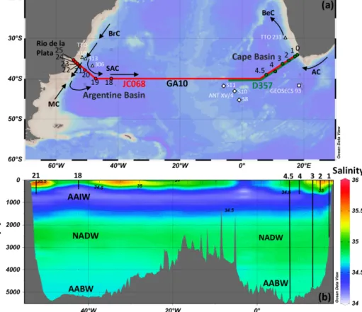
The study was conducted from the RRSDiscoveryand RRS James Cookduring two UK GEOTRACES cruises, D357 and JC068, along the GA10 40^◦S transect of the Atlantic Ocean (Fig. 1). The surface currents show dynamic interaction and mixing on both the western and eastern sides of this transect. In the Argentine Basin, the Río de la Plata estuary is located on the western margin of the transect. The boundary Brazil Current (BrC) and Malvinas Current (MC) meet between 33 and 45^◦S along the continental margin of South America and these become the South Atlantic Current (SAC) transporting water eastwards along 40^◦S. The water from the BrC is captured between Stn20 and Stn21 with a strong west to east gradient in salinity and other chemical and physical properties, which also suggests a limited exchange of water across the continental shelf break (see below). In the Cape Basin, the SAC turns northeast before reaching the continent of Africa, and the Agulhas Current (AC) adds warm water eddies from the Indian Ocean. The warm and salty water of the AC was sampled in the top 500 m at Stn2 (Fig. 1b). These currents meet and become the Benguela Current (BeC) flowing through the Cape Basin and into the South Atlantic.

2.2 Water sampling

Seawater samples for Ra analysis were collected from 14 stations on the D357 and JC068 cruises (Fig. 1). The first

(3)

Figure 1. (a)Map of cruise tracks, station locations and surface currents. GA10 cruise D357 and JC068 stations are labelled with green and red circles, respectively. Stations of previous Ra studies are labelled with open symbols (Transient Tracers in the Ocean (TTO): Key et al., 1990, 1992a, b; GEOSECS: Ku and Lin, 1976; ANT XV/4: Hanfland, 2002). Surface currents are shown with arrows.(b)Salinity profiles along the cruise track of UK GEOTRACES GA10 are labelled with water masses. Vertical lines indicate the stations where vertical Ra water profiles are available.

cruise (D357) took place in the SE Atlantic (Cape Basin) between October and November 2010; the second cruise (JC068) took place along the whole 40^◦S transect between December 2011 and January 2012. For radium isotope analyses, the Cape Basin samples were only taken from D357, and the Argentine Basin samples were taken from JC068.

For TEs, samples were taken from both D357 and JC068.

Stations from these cruises are shown along with those from previous Ra studies (e.g. GEOSECS and TTO) in this region (Fig. 1a).

A total of 48 samples were analysed for ²²⁸Ra/²²⁶Ra ratio and ²²⁸Ra concentration, and 33 samples for ²²⁶Ra concentration, collected using three different sampling techniques during the cruise. Surface seawater samples (80–

100 L) at 5 m depth were collected via a trace-metal clean seawater supply (fish) using a Teflon bellow pump (Almatec- A15) and acid-cleaned tubing. Samples between 50 and 400 m were collected using a standard conductivity, temperature, and depth (CTD) rosette, typically sampling from four 20 L Niskin bottles. These samples were stored briefly in low-density polyethylene (LDPE) cubitainers and then filtered through Mn-fibre cartridges by gravity (flow rate

<0.5 L min⁻¹) on board for the extraction of radium iso-

topes (Moore et al., 1985; Reid et al., 1979). In addition, large-volume seawater sampling (300–600 L) was carried out using in situ stand-alone pump (SAP) systems, pumping seawater over Mn fibres in polypropylene cartridges (van Beek et al., 2008) at flow rate of 2–5 L min⁻¹ at three selected sampling stations (Stn1, Stn3, and Stn4.5). As the cartridge Ra collection efficiency varies hugely, ranging from 70 % to 128 % (Geibert et al., 2013), all samples collected by these collection techniques (pump, CTD, and SAP) were only used for measurement of²²⁸Ra/²²⁶Ra ratios. To address the efficiency issue, for most samples, a separate sample of 250 mL seawater was also collected for measurement of²²⁶Ra concentration. This method provides the advantage of allowing a correction for variable efficiencies during the sample prepa- ration.

Trace element samples were collected using a tita- nium CTD rosette fitted with trace-metal clean Teflon- coated Niskin bottles and filtered on board through 0.8/0.2 µm polyethersulfone (PES) membrane cartridge fil- ters (AcroPak500™, Pall) before analysis. All the TE data and fluxes reported and discussed in this study refer to the dissolved fraction only. The data of zinc and cobalt were measured and published by Wyatt et al. (2014, 2020). Some

(4)

of the iron data were determined and published by Brown- ing et al. (2014) and Clough et al. (2016). All the TE data are available on the GEOTRACES Intermediate Data Prod- uct (IDP) 2017 (Schlitzer et al., 2018).

All the trace-metal cleaning procedures followed the GEOTRACES sampling protocols (Cutter et al., 2010). In brief, the sample tubing and bottles were rinsed with Milli- Q water and filled with 0.1 M HCl for 1 d. After emptying the acid, the tubing and bottles were rinsed thoroughly with Milli-Q water. The tubing and bottles were also rinsed with open-ocean seawater before sampling.

2.3 Ra isotopes analysis

Mn-fibre samples were first counted on board using a four- channel radium delayed coincidence counting (RaDeCC) system for ²²⁴Ra, ²²³Ra, ²²⁸Th, and ²²⁷Ac (Moore and Arnold, 1996), but the data for ²²⁴Ra, ²²³Ra, ²²⁸Th, and

227Ac are not discussed in this paper. After the counting, Ra was purified using the following procedure for precisely measuring²²⁸Ra/²²⁶Ra ratios and²²⁸Ra concentrations by a Nu Instrument multi-collector inductively coupled plasma mass spectrometry (MC-ICP-MS) at the University of Ox- ford following the procedures established by Hsieh and Hen- derson (2011). Mn fibres were ashed at 550^◦C for 6 h and then leached with distilled 6 N HCl to remove Ra from the ashed fibres. Ra was then co-precipitated with Sr(Ra)SO4in the leached solution, centrifuged, and cleaned with 3 N HCl and pure H2O a few times until the pH was>4. To increase the dissolution rate, Sr(Ra)SO4was converted to Sr(Ra)CO3

by adding 2 mL 1 M Na2CO3 solution and heated on a hot- plate for 3 h. After centrifuging and discarding the super- natant, Sr(Ra)CO₃was finally dissolved in 2 mL 6 N HCl for ion exchange column chemistry, using Bio-Rad AG50-X8 cation exchange resin (to separate Ra and Ba from²²⁸Th and other matrix elements, e.g. Ca, Sr, and Mn) and Eichrom Sr- Spec resin (to separate Ra from Ba to avoid molecular inter- ferences during MC-ICP-MS analysis).

Smaller seawater samples (250 mL) collected for ²²⁶Ra were spiked with a²²⁸Ra spike (Hsieh and Henderson, 2011) and the Ra was purified by the precipitation of CaCO₃and processing with ion exchange columns of AG1-X8, AG50- X8, and Sr-Spec resin for the measurement of²²⁶Ra concentrations by MC-ICP-MS (Foster et al., 2004). In general, the contribution of seawater²²⁸Ra (<0.05 attomole) is negligible, compared to the spiked ²²⁸Ra signal (≈70 attomole).

Assessments of overall chemical blanks were conducted the same way as for the samples throughout the whole chemical procedures, except that there was no added seawater. The blanks were found to contribute less than 1 % of the²²⁶Ra in the sample and were not detectable for²²⁸Ra.

During the MC-ICP-MS analyses,²²⁸Ra and²²⁶Ra were measured simultaneously on two ion counters, and the ura- nium standard CRM-145 was used to bracket each sample for the mass bias and ion counter gain corrections. Instrumental

memories of²²⁸Ra and²²⁶Ra were also detected on ion counters before each measurement. The machine memory was about 0.2±0.1 cps (counts per second) (n=16, 2 SE). The memory correction was insignificant for²²⁶Ra, because the ratio of memory to sample signal is small (<10⁻⁴). How- ever, the memory correction could be significant for samples with low²²⁸Ra activities and count rates. For instance, the count rate during analysis of²²⁸Ra on the sample collected at 4741 m at Stn4.5 was only 0.5 cps. At this low count rate, instrumental memory contributed∼40 % of the signal to the sample²²⁸Ra signal and the uncertainty of memory correction becomes substantial. In this study, most of the surface and deep waters in the South Atlantic were measured at count rates>2 cps²²⁸Ra, which provides assurance that the contribution of the instrumental memory uncertainty to the total uncertainty is<10 %.

For samples without accompanied ²²⁶Ra measurements, silica data (Table 1) are used to assess²²⁶Ra activities (Ap- pendix A). The Atlantic Ocean²²⁶Ra–Si relationship is based on the GEOTRACES (GA03), GEOSECS, and TTO datasets (Fig. A1 in Appendix A, Ku and Lin, 1976; Key et al., 1990, 1992a, b; Charette et al., 2015). This relationship is used to determine²²⁶Ra activities in the 27 cases where no subsam- ples were collected for separate²²⁶Ra analysis (such²²⁶Ra estimates are shown in brackets in Table 1). The relationship has a slope of 0.119 dpm 100 L⁻¹of²²⁶Ra per µmol L⁻¹ of Si and an intercept of 8.8 dpm 100 L⁻¹, which is comparable with the average slope of 0.1 observed by Broecker et al. (1976) in the Atlantic. The Si-extrapolated²²⁶Ra and measured²²⁶Ra activities (data from this study and the TTO) show a relatively consistent result although the extrapolated

226Ra has a larger uncertainty (±11 % 2 SE) than the measured ²²⁶Ra uncertainty (±4 %, 2 SE). The paired t test shows a p value of 0.55 (>0.05), suggesting that the dif- ferences between the extrapolated²²⁶Ra and the measured

226Ra data are not statistically significant. The uncertainties of ²²⁶Ra activity have been used in the error propagation of²²⁸Ra activity; the total uncertainty of²²⁸Ra is typically about 6 %–12 % (2 SE).

2.4 ²²⁸Ra-derived 1-D mixing models

The distribution of seawater ²²⁸Ra in the ocean is mainly controlled by mixing, advection, radioactive decay, and additional removal/input. It has been widely used as a tracer for measuring diffusion coefficients and advection rates on a basin-wide scale in the surface or at intermediate depths in the ocean (e.g. Cochran, 1992; Ku and Luo, 2008; Sanial et al., 2018). The one-dimensional (1-D)²²⁸Ra advection–

diffusion model is commonly expressed by the following for- mula (e.g. Moore, 2015):

∂A

∂t =Kx

∂²A

∂x² −w∂A

∂x −λA±J, (1)

(5)

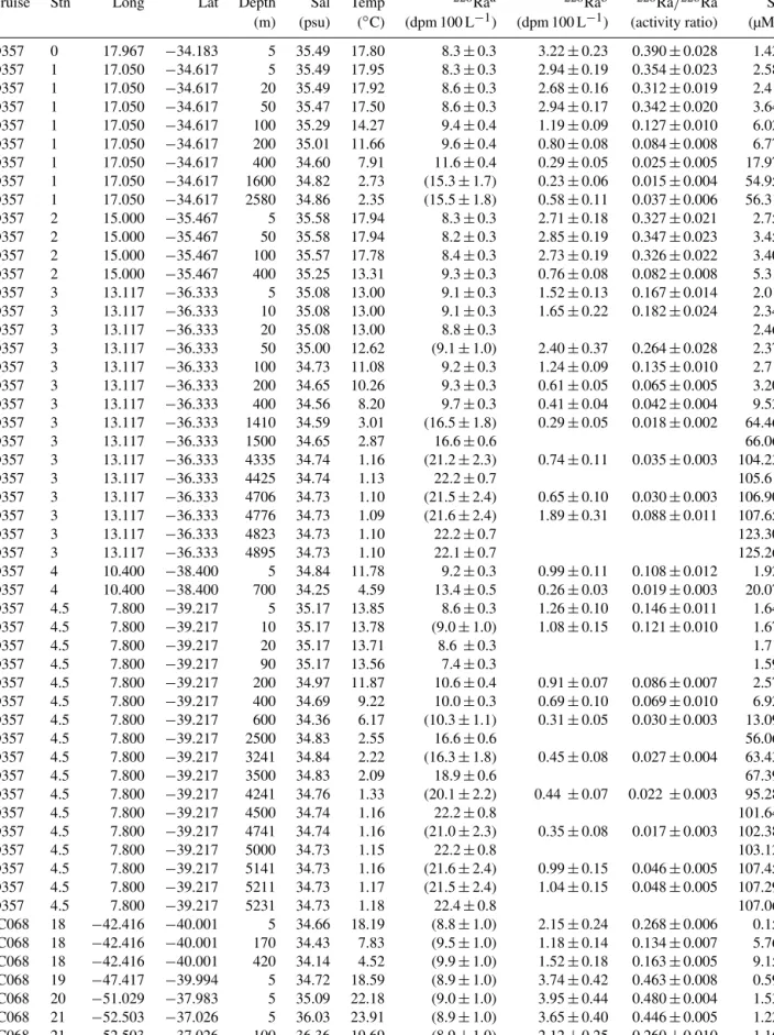
Table 1.²²⁶Ra and²²⁸Ra activities,²²⁸Ra/²²⁶Ra activity ratios, and silica concentration.

Cruise Stn Long Lat Depth Sal Temp ²²⁶Ra^a ²²⁸Ra^b ²²⁸Ra/²²⁶Ra Si

(m) (psu) (^◦C) (dpm 100 L⁻¹) (dpm 100 L⁻¹) (activity ratio) (µM)

D357 0 17.967 −34.183 5 35.49 17.80 8.3±0.3 3.22±0.23 0.390±0.028 1.42

D357 1 17.050 −34.617 5 35.49 17.95 8.3±0.3 2.94±0.19 0.354±0.023 2.58

D357 1 17.050 −34.617 20 35.49 17.92 8.6±0.3 2.68±0.16 0.312±0.019 2.41 D357 1 17.050 −34.617 50 35.47 17.50 8.6±0.3 2.94±0.17 0.342±0.020 3.64 D357 1 17.050 −34.617 100 35.29 14.27 9.4±0.4 1.19±0.09 0.127±0.010 6.02 D357 1 17.050 −34.617 200 35.01 11.66 9.6±0.4 0.80±0.08 0.084±0.008 6.77 D357 1 17.050 −34.617 400 34.60 7.91 11.6±0.4 0.29±0.05 0.025±0.005 17.97 D357 1 17.050 −34.617 1600 34.82 2.73 (15.3±1.7) 0.23±0.06 0.015±0.004 54.95 D357 1 17.050 −34.617 2580 34.86 2.35 (15.5±1.8) 0.58±0.11 0.037±0.006 56.31

D357 2 15.000 −35.467 5 35.58 17.94 8.3±0.3 2.71±0.18 0.327±0.021 2.75

D357 2 15.000 −35.467 50 35.58 17.94 8.2±0.3 2.85±0.19 0.347±0.023 3.45 D357 2 15.000 −35.467 100 35.57 17.78 8.4±0.3 2.73±0.19 0.326±0.022 3.40 D357 2 15.000 −35.467 400 35.25 13.31 9.3±0.3 0.76±0.08 0.082±0.008 5.31

D357 3 13.117 −36.333 5 35.08 13.00 9.1±0.3 1.52±0.13 0.167±0.014 2.01

D357 3 13.117 −36.333 10 35.08 13.00 9.1±0.3 1.65±0.22 0.182±0.024 2.34

D357 3 13.117 −36.333 20 35.08 13.00 8.8±0.3 2.46

D357 3 13.117 −36.333 50 35.00 12.62 (9.1±1.0) 2.40±0.37 0.264±0.028 2.37 D357 3 13.117 −36.333 100 34.73 11.08 9.2±0.3 1.24±0.09 0.135±0.010 2.71 D357 3 13.117 −36.333 200 34.65 10.26 9.3±0.3 0.61±0.05 0.065±0.005 3.20 D357 3 13.117 −36.333 400 34.56 8.20 9.7±0.3 0.41±0.04 0.042±0.004 9.52 D357 3 13.117 −36.333 1410 34.59 3.01 (16.5±1.8) 0.29±0.05 0.018±0.002 64.46

D357 3 13.117 −36.333 1500 34.65 2.87 16.6±0.6 66.06

D357 3 13.117 −36.333 4335 34.74 1.16 (21.2±2.3) 0.74±0.11 0.035±0.003 104.23

D357 3 13.117 −36.333 4425 34.74 1.13 22.2±0.7 105.61

D357 3 13.117 −36.333 4706 34.73 1.10 (21.5±2.4) 0.65±0.10 0.030±0.003 106.90 D357 3 13.117 −36.333 4776 34.73 1.09 (21.6±2.4) 1.89±0.31 0.088±0.011 107.65

D357 3 13.117 −36.333 4823 34.73 1.10 22.2±0.7 123.30

D357 3 13.117 −36.333 4895 34.73 1.10 22.1±0.7 125.26

D357 4 10.400 −38.400 5 34.84 11.78 9.2±0.3 0.99±0.11 0.108±0.012 1.92

D357 4 10.400 −38.400 700 34.25 4.59 13.4±0.5 0.26±0.03 0.019±0.003 20.07 D357 4.5 7.800 −39.217 5 35.17 13.85 8.6±0.3 1.26±0.10 0.146±0.011 1.64 D357 4.5 7.800 −39.217 10 35.17 13.78 (9.0±1.0) 1.08±0.15 0.121±0.010 1.67

D357 4.5 7.800 −39.217 20 35.17 13.71 8.6±0.3 1.71

D357 4.5 7.800 −39.217 90 35.17 13.56 7.4±0.3 1.59

D357 4.5 7.800 −39.217 200 34.97 11.87 10.6±0.4 0.91±0.07 0.086±0.007 2.57 D357 4.5 7.800 −39.217 400 34.69 9.22 10.0±0.3 0.69±0.10 0.069±0.010 6.92 D357 4.5 7.800 −39.217 600 34.36 6.17 (10.3±1.1) 0.31±0.05 0.030±0.003 13.09

D357 4.5 7.800 −39.217 2500 34.83 2.55 16.6±0.6 56.06

D357 4.5 7.800 −39.217 3241 34.84 2.22 (16.3±1.8) 0.45±0.08 0.027±0.004 63.43

D357 4.5 7.800 −39.217 3500 34.83 2.09 18.9±0.6 67.39

D357 4.5 7.800 −39.217 4241 34.76 1.33 (20.1±2.2) 0.44±0.07 0.022 ±0.003 95.28

D357 4.5 7.800 −39.217 4500 34.74 1.16 22.2±0.8 101.64

D357 4.5 7.800 −39.217 4741 34.74 1.16 (21.0±2.3) 0.35±0.08 0.017±0.003 102.38

D357 4.5 7.800 −39.217 5000 34.73 1.15 22.2±0.8 103.12

D357 4.5 7.800 −39.217 5141 34.73 1.16 (21.6±2.4) 0.99±0.15 0.046±0.005 107.45 D357 4.5 7.800 −39.217 5211 34.73 1.17 (21.5±2.4) 1.04±0.15 0.048±0.005 107.29

D357 4.5 7.800 −39.217 5231 34.73 1.18 22.4±0.8 107.06

JC068 18 −42.416 −40.001 5 34.66 18.19 (8.8±1.0) 2.15±0.24 0.268±0.006 0.15 JC068 18 −42.416 −40.001 170 34.43 7.83 (9.5±1.0) 1.18±0.14 0.134±0.007 5.76 JC068 18 −42.416 −40.001 420 34.14 4.52 (9.9±1.0) 1.52±0.18 0.163±0.005 9.15 JC068 19 −47.417 −39.994 5 34.72 18.59 (8.9±1.0) 3.74±0.42 0.463±0.008 0.59 JC068 20 −51.029 −37.983 5 35.09 22.18 (9.0±1.0) 3.95±0.44 0.480±0.004 1.53 JC068 21 −52.503 −37.026 5 36.03 23.91 (8.9±1.0) 3.65±0.40 0.446±0.005 1.22 JC068 21 −52.503 −37.026 100 36.36 19.69 (8.9±1.0) 2.12±0.25 0.260±0.010 1.16

(6)

Table 1.Continued.

Cruise Stn Long Lat Depth Sal Temp ²²⁶Ra^a ²²⁸Ra^b ²²⁸Ra/²²⁶Ra Si

(m) (psu) (^◦C) (dpm 100 L⁻¹) (dpm 100 L⁻¹) (activity ratio) (µM) JC068 21 −52.503 −37.026 200 35.81 16.43 (9.0±1.0) 2.84±0.33 0.344±0.012 1.86 JC068 21 −52.503 −37.026 600 34.56 7.85 (10.1±1.1) 1.02±0.12 0.107±0.004 10.66 JC068 22 −53.102 −36.538 5 30.26 23.00 (10.0±1.1) 13.55±1.49 1.441±0.008 9.80 JC068 23 −53.337 −36.338 5 29.62 23.35 (10.0±1.1) 14.08±1.55 1.469±0.008 11.04 JC068 24 −54.000 −36.000 5 28.48 23.06 (11.3±1.2) 17.66±1.95 1.599±0.011 21.22 JC068 25 −54.560 −35.493 5 30.61 23.04 (9.2±1.0) 12.76±1.41 1.497±0.013 3.68

aRa-226 activity in brackets is extrapolated from the²²⁶Ra–silica relationship in Fig. A1.^bRa-228 activity is calculated from the activity ratio of²²⁸Ra/²²⁶Ra multiplied by²²⁶Ra activity. All errors are 2 standard errors.

whereAis activity of²²⁸Ra,t is time,K_xis horizontal eddy diffusion coefficient, w is advection velocity, x is offshore distance,λis decay constant (λ_Ra228=3.82×10⁻⁹s⁻¹), and J is additional input or removal of²²⁸Ra.

To use the model to accurately calculate the mixing rates, several assumptions need to be made.

2.4.1 Steady state (∂A/∂t=0)

This assumption requires long-term monitoring of ²²⁸Ra activities in the ocean due to the long half-life of ²²⁸Ra.

Charette et al. (2015) compared the²²⁸Ra data in the North Atlantic from the US GEOTRACES and the TTO pro- grammes, and found that the upper ocean ²²⁸Ra invento- ries have remained constant over the past 30 years. Although

228Ra seasonality in coastal areas may introduce uncertainty to the mixing model, the assumption of steady state is likely to be valid for²²⁸Ra on decadal timescales and at ocean basin scales. The comparison between our²²⁸Ra data and the limited data from the TTO in this region shows good agreement (Fig. 2b), supporting this assumption for the South Atlantic.

2.4.2 No additional input or removal of²²⁸Ra (±J=0) Based on particle removal, Ra residence time is estimated to be ∼500 years in the surface ocean (Moore and Dymond, 1991). However, there is no measurable particle removal of Ra in the surface open ocean at the timescale of²²⁸Ra half- life (5.75 years) (Moore, 2015). In theory, the distribution of seawater²²⁸Ra is controlled by both vertical and horizontal mixing. For example, vertical mixing could potentially introduce additional “removal” of²²⁸Ra from the surface water and affect the horizontal distribution of²²⁸Ra in the surface ocean, which would require 2-D models and a high sample resolution dataset to resolve the problem. However, vertical mixing (∼0.1–1 cm²s⁻¹) is typically 5 to 8 orders of magnitude smaller than horizontal mixing (∼10⁵–10⁷cm²s⁻¹), and the sample resolution is not good enough for precise 2- D modelling in this study. Therefore, we only apply the 1-D model to estimate the maximum horizontal mixing rates by neglecting the term of downward mixing.

Similar assumptions need to be made for the²²⁸Ra-derived vertical mixing – the gradient of²²⁸Ra with depth mainly re- flects the vertical mixing rates, and the vertical²²⁸Ra distribution is not affected by additional input of horizontal²²⁸Ra below the mixed layer. These assumptions are mostly true in the upper open ocean, where horizonal²²⁸Ra mainly comes from the continental margins (shelf and slope sediments) and there is a lack of other important²²⁸Ra sources in the middle of the ocean. However, if the lateral input becomes important and starts to interfere with the²²⁸Ra vertical profiles (e.g. re- ceiving strong advective shelf water or profiles closer to the seafloor), the 1-D²²⁸Ra-derived vertical mixing rates can be significantly overestimated.

2.4.3 Boundary conditions (A=A₀atx=0 andA=0 atx→ ∞)

It has been pointed out that the boundary condition ofA=0 atx→ ∞is incorrect for using²²⁸Ra to determine coastal mixing as the distribution of ²²⁸Ra could be controlled by water mass mixing within the coastal distance scale (<

50 km) rather than eddy diffusion (Moore, 2000). In theory, this boundary condition may be valid on the ocean basin scale, as the major sink of ²²⁸Ra in the ocean is radioactive decay. However, observed seawater ²²⁸Ra is still not completely zero in the remote ocean. To avoid this problem, we follow the suggestion of Moore (2015) and define the²²⁸Ra excess (²²⁸Raex=²²⁸Ra−²²⁸Rabg) by subtracting the background value in the middle of the South Atlantic,

228Rabg: 0.23±0.06 dpm 100 L⁻¹(1 SE,n=6). This value is determined by the average of the observed values at (1) the remote surface waters in a previous study around the 40^◦S transect (Hanfland, 2002; Fig. 1, ANT XV/4 station S8, S10, and S11); and (2) the water depth between 1000 and 3500 m in this study (except for 2580 m at Stn1 on the continental slope). The mid-depth²²⁸Ra background (1000–

3500 m) shares a similar background as the remote surface waters (∼0.2 dpm 100 L⁻¹), suggesting that the²²⁸Ra background needs to be corrected in both horizontal and vertical mixing calculations. For comparison, the central North Atlantic shows a similar mid-depth²²⁸Ra background value

(7)

(∼0.16 dpm 100 L⁻¹) between 1000 and 3000 m depth from the GEOTRACES GA03 transect (Stn12–20; Charette et al., 2015). However, the surface value in the central North At- lantic (∼2.2 dpm 100 L⁻¹) is significantly higher than that in the South Atlantic (∼0.2 dpm 100 L⁻¹), which has also been observed by Moore et al. (2008). We therefore use a background value of ²²⁸Ra_bg: 0.23±0.06 dpm 100 L⁻¹ determined from the South Atlantic.

The boundary condition can now be rewritten asA_{ex_0}= A₀−A_bg atx=0 and A_ex=0 atx= ∞. Considering the assumptions discussed above, Eq. (1) can be written as 0=K_x∂²A_ex

∂x² −w∂A_ex

∂x −λAex. (2)

In this study, we consider two scenarios in the horizontal

228Ra calculations: (1) mixing only (w=0) and (2) advection only (K_x=0). We use these two scenarios to provide independent assessments of chemical fluxes in the surface ocean, to bracket the range of possible TE fluxes that are consistent with the²²⁸Ra data regardless of the combination of mixing and advection in the real ocean. The advection model is only applied to the Argentine Basin data after the shelf break where the advection signal is strong because of the Brazil Current. Although the advection only scenario is an unrealistic one, it provides an end-member for comparisons of TE fluxes under different settings. Using the boundary conditions,A_{ex_0}=A₀−A_bgatx=0 andA_ex=0 atx= ∞, Eq. (2) can be solved for diffusive mixing only:

Aex=Aex_0exp(−ax) , where a=p

λ/Kx, (3)

and for advection only:

w=λx/ln(Aex_0/Aex)=X1/2/T1/2, (4) whereA_{ex_0}is the activity of²²⁸Ra_exatx=0 (i.e. Stn0 or Stn25); X_1/2 is the distance at whichA_ex=0.5A_{ex_0}; and T_1/2is the half-life of²²⁸Ra (5.75 years). The exponential fit of the surface²²⁸Ra data provides the estimate of the maximum diffusion coefficients (Kx) at both ends of the transect, and the linear fit of the surface²²⁸Ra data after the shelf break in the Argentine Basin provides the minimum estimate of the advection water transport (w) along the west end of the transect (see discussion below).

For vertical mixing, the calculation of Kz is based on a situation in which ²²⁸Ra is mixed horizontally away from the coast in the surface mixed layer and then down into the subsurface. The 1-D mixing model can therefore be applied to the depth profiles of²²⁸Ra to calculateK_znear the surface ocean. Under similar boundary conditionsA_{ez_0}=A₀−A_bg atz=0 andA_ez=0 atz= ∞, the diffusion equation can be solved for vertical mixing to fit the vertical²²⁸Ra profiles:

Aez=Aez_0exp(−az) , where a=p

λ/Kz, (5)

whereA_{ez_0}is the activity of²²⁸Ra_exatz=0 (i.e. the mixed layer). In the 1-D mixing model, the term for diapycnal ad-

vection is generally negligible, as the oceanic vertical advection velocity is usually very small, i.e. 10⁻³–10⁻⁵cm s⁻¹ (Liang et al., 2017).

2.5 Trace element flux calculations

In this study, we use three different ²²⁸Ra approaches to quantify the horizontal and diffusive vertical dTE fluxes in the Cape Basin and Argentine. More details of the calculations are provided in Appendix D.

2.5.1 ²²⁸Ra-derived diffusive TE fluxes

To calculate both lateral and vertical TE fluxes, the²²⁸Ra- derived diffusion coefficients (KzorKx) are applied to Fick’s first law of molecular diffusion in the following equation:

FTE−d=Kxorz(1TE/1xor1z) , (6) whereF_TE−dis the diffusive flux of the TEs, and1TE/1x or1zis the gradient of TE concentration over either the horizontal distancexto the coasts or the vertical depthzbelow the mixed layer, which can be obtained from the linear regression of horizontal and vertical TE profiles (Sect. 3.2).

2.5.2 ²²⁸Ra-derived advective TE fluxes

Surface water after the boundary of the shelf break and the Brazil Current in the Argentine Basin carries strong offshore advection signals along the SAC towards the open ocean (Fig. 1). Assuming that the mixing of TE is conservative, the advective TE fluxes can be calculated using the following equation:

F_TE−a=w·[TE]_ave−0, (7)

whereF_TE−a is the offshore advective flux of TE, wis the net offshore advection velocity along the SAC in the Argen- tine Basin, and [TE]_ave−0 is the average concentrations of dissolved TEs in the initial advective waters around where the Brazil Current merges into the SAC (around Stn21).

2.5.3 TE/²²⁸Ra-ratio-derived TE fluxes

Previous studies have combined the use of the shelf²²⁸Ra fluxes with the ratios of TE/²²⁸Ra in the surface waters between continental shelves and open oceans to estimate the shelf–ocean TE inputs from the continental margins to the open oceans (Charette et al., 2016; Sanial et al., 2018; Vieira et al., 2020). This method provides the integrated net fluxes of TEs, considering all the possible inputs (e.g. rivers, SGD, and sediments) and outputs (e.g. particle scavenging, biological uptake, and radioactive decay) of²²⁸Ra and TEs during water mixing between the continental shelf and the open ocean. More details of the method are given in Charette et al. (2016). In brief, assuming that the net shelf–ocean exchange is mainly driven by eddy diffusion, the cross-shelf

(8)

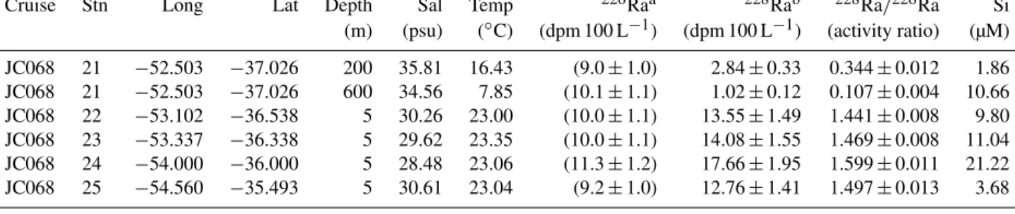
Figure 2.Depth profiles of(a)²²⁶Ra and(b)²²⁸Ra activities. The grey squares show Ra data from the previous GEOSECS study (Ku and Lin, 1976); the triangles show Ra data from the TTO programme (Key et al., 1990, 1992a, b). Different water masses are characterised in the (a)²²⁶Ra profile (see details in text). Error bars are±2 SE.

TE fluxes can be calculated using the following equation:

F_TE=F_228Ra·

1TE 1²²⁸Ra

=F_228Ra·

TE_shelf−TE_ocean

228Ra_shelf−²²⁸Ra_ocean

, (8)

where F_228Ra is the cross-shelf ²²⁸Ra flux (Appendix D);

TE_shelf and²²⁸Ra_shelf are the average concentrations of the TE and ²²⁸Ra in the surface waters on the shelf (GA10W:

between Stn23 and Stn25; GA10E: between Stn0 and Stn1), respectively; and TEoecanand²²⁸Raoceanare the average concentrations in the open ocean (GA10W: between Stn18 and Stn19; GA10E: between Stn4 and Stn4.5). The ratios of 1TE/1²²⁸Ra are reported in Table D1 in Appendix D.

3 Results

3.1 Ra isotope concentrations

The results of²²⁶Ra and²²⁸Ra activities and the activity ratios of²²⁸Ra/²²⁶Ra are presented in Table 1 (with±2 SE).

The vertical profiles of measured ²²⁶Ra show good agreement with the data from the closest GEOSECS and TTO stations in this region (e.g. Ku and Lin, 1976; Key et al., 1990, 1992a, b) (Fig. 2a). Ra-226 activities range from 8.2 to 22.4 dpm 100 L⁻¹. In this study, the results of ²²⁶Ra are mainly used for calculating²²⁸Ra activities, and will not be discussed in further detail.

The activity ratios of ²²⁸Ra/²²⁶Ra range from 0.017 to 1.599 in the surface water and are comparable with

the ratios from 0.080 to 2.810 observed in previous studies in this region (TTO data, Windom et al., 2006; Han- fland, 2002). The vertical profiles of ²²⁸Ra activity are shown in Fig. 2b. In surface waters, the activities of²²⁸Ra ranging from 1.02 to 17.66 dpm 100 L⁻¹ in the Argentine Basin are consistent with the observed values from 0.07 to 24.0 dpm 100 L⁻¹ from the previous studies (TTO data and Windom et al., 2006), and the activities of ²²⁸Ra ranging from 0.99 to 3.22 dpm 100 L⁻¹in the Cape Basin are consistent with the observed values from 0.67 to 4.23 dpm 100 L⁻¹ from the previous study (Hanfland, 2002). Between 600 and 4000 m, ²²⁸Ra/²²⁶Ra ratios decrease to 0.015–0.030 and ²²⁸Ra activities decrease to 0.29–0.32 dpm 100 L⁻¹. In the 100 m closest to the ocean floor, the ratios of

228Ra/²²⁶Ra increase to 0.048–0.088 and the activities of

228Ra also increase to 1.07–1.94 dpm 100 L⁻¹. This is the first dataset of seawater ²²⁸Ra reported in the intermediate and deep waters in the Cape Basin. The ²²⁸Ra values in the Cape Basin are noticeably higher than those observed in intermediate (<0.1 dpm 100 L⁻¹) and deep waters (0.22–0.28 dpm 100 L⁻¹) to the south in the Southern Ocean (Charette et al., 2007; van Beek et al., 2008). The vertical profiles of seawater²²⁸Ra in the Cape Basin are consistent with GEOSECS and TTO observations elsewhere in the South Atlantic Ocean (Moore et al., 1985). The samples collected by pump (fish), CTD, and SAP within the mixed layer at each station show consistent²²⁸Ra and²²⁶Ra results, suggesting that there is no significant difference in the Ra results between these three sampling methods.

(9)

3.2 Micronutrient concentrations

Dissolved Co, Fe, and Zn concentration data (Wyatt et al., 2014, 2020; Browning et al., 2014; Clough et al., 2016;

Schlitzer et al., 2018) are summarised in Appendix B (Ta- bles B1 and B2). At the continental margins, surface shelf waters show much higher trace element concentrations (Co:

146.2 pM, Fe: 1.53 nM, and Zn: 0.59 nM in the Argentine Basin margin; Co: 46.9 pM, Fe: 0.35 nM, and Zn: 0.14 nM in the Cape Basin margin) than observed in the open-ocean surface waters along the 40^◦S transect (Fig. 3). In the Argentine Basin, the distribution of trace elements generally follows the salinity in the surface waters. The low-salinity waters (<

29 psu) around 200 km from the South America coast show high TE concentrations (Co:>80 pM, Fe:>1 nM, and Zn:

>0.5 nM). In contrast, the high-salinity waters (>35 psu) in the Brazil Current show much lower TE concentrations (Co:

<60 pM, Fe:<0.5 nM, and Zn:<0.2 nM). Similar correla- tions between trace elements and salinity have been observed along other western boundaries of the Atlantic as well (e.g.

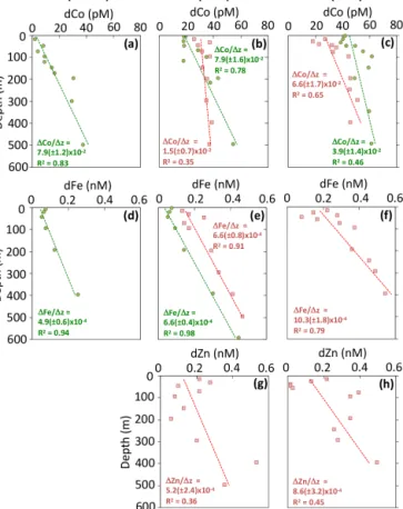
the North American shelf; Bruland and Franks, 1983; Noble et al., 2017). In the upper ocean (<600 m), these trace element concentrations are generally low in the surface mixed layer and increase with depth below the mixed layer (Fig. 4).

Co concentrations range from 1.6 to 61.2 pM, and Fe and Zn concentrations range from 0.05 to 0.54 and 0.01 to 0.53 nM, respectively. In general, these trace element concentrations (<600 m) are slightly higher in Stn1 than other stations further away from the continental shelf.

4 Discussion

4.1 ²²⁸Ra-derived horizontal mixing and advection 4.1.1 Argentine Basin

The distribution of²²⁸Ra_exin the Argentine Basin (GA10W) is controlled by the Rio de la Plata river plume and the Brazil Current (Fig. 5a), and this is supported by a good correlation with salinity (linear regression R²=0.96; Fig. C1 in Ap- pendix C). If we apply the 1-D mixing model (Eq. 3) to fit the

228Raexdata between Stn25 and Stn21, across the boundary of the Brazil Current, the gradient of the exponential fit (a) is 0.0047±0.0027 and the estimate of the offshore horizontal diffusion coefficientKxis 1.8±1.4×10⁶cm²s⁻¹, which is likely to be an overestimate due to the influence of the river plume and the advection of the boundary current. Neverthe- less, this estimate is still within the range of other estimates of K_x between 10⁵and 10⁸cm²s⁻¹in a variety of margin and open-ocean settings (e.g. Kaufman et al., 1973; Knauss et al., 1978; Yamada and Nozaki, 1986).

Across the boundary of the Brazil Current, the advection of the eastward flowing SAC shows a significant im- pact on the distribution of ²²⁸Ra_ex in the surface Argen- tine Basin (Fig. 5a). If we apply the 1-D advection model

(Eq. 4) to fit the data between Stn21 and Stn18 (Fig. 5a), theX1/2is 1116±600 km (from Stn 21) and the estimate of average advection velocitywis 0.6±0.3 cm s⁻¹. Although the ²²⁸Ra-derived velocity is smaller than the typical ve- locities (2–4 cm s⁻¹) around the South Atlantic subtropical gyre (Schlitzer, 1996), similar advective²²⁸Ra signals have been previously observed in other surface ocean current systems, including the Peru and Kuroshio currents in the Pacific (Knauss et al., 1978; Yamada and Nozaki, 1986).

4.1.2 Cape Basin

Ra-228 data from the Cape Basin transect (GA10E) are used to calculate the offshore horizontal diffusion coefficient (Kx) in the Cape Basin (Fig. 5b). Applying the simple 1- D mixing model, assumingw=0, to fit the surface²²⁸Raex

data in the Cape Basin (Fig. 5b), the gradient of the exponential fit (a) is 0.0012±0.0003 and the estimate of Kx

is 2.7±0.8×10⁷cm²s⁻¹, which is an order of magnitude higher than the value observed in the Argentine Basin (see above) but within the range of other observed values in the oceans (10⁵–10⁸cm²s⁻¹).

The horizontal diffusion coefficientK_xis likely to be overestimated in the Cape Basin due to the influence of episodic water advection. The Agulhas Current leakage (ACL) is known for transporting water from the Indian Ocean into the South Atlantic and episodically introduces eddies (Agulhas rings) into the Cape Basin (Beal et al., 2011). However, the signals of mixing and advection cannot be easily separated with the²²⁸Ra data alone (Fig. 5b). For example, the distribution of²²⁸Raexin the surface Cape Basin shows elevated values (Stn2 and Stn4.5) above the fitted curve and coincides with the elevated salinity and temperature data (Fig. 5d), which indicates that the elevated²²⁸Ra_ex is likely to come from an advective signal (e.g. ACL). The ACL signal has also been identified with a distinct Pb isotope signature in the upper water column at Stn2 (Paul et al., 2015). The application of a 1-D mixing model may actually be biased by the addition of these high²²⁸Ra_exwaters; therefore, the horizontal diffusion coefficientK_x is likely to be a maximum estimate for the Cape Basin. Nevertheless, the overall gradient of²²⁸Raex, decreasing along the distance away from the shore, is driven by the loss of²²⁸Ra through both water mixing and radioactive decay.

Despite uncertainty in the diffusion coefficients due to advection of other sources, the²²⁸Ra data do place bounds on maximum horizontal mixing in the surface ocean away from the eastern and western boundaries of the Atlantic at 40^◦S.

These bounds can be used to quantify the trace element inputs from the continental margins to the South Atlantic (see Sect. 4.3).

(10)

Figure 3.Dissolved trace elements (dCo, dFe, and dZn) and salinity in the surface water (<10 m) along the 40^◦S Argentine and Cape Basin transects. Red squares show data from cruise JC068, and green circles show data from cruise D357. The orange band indicates the boundary of the BrC in the Argentine Basin transect, highlighted by high salinity and changing TE gradients. [TE]_ave−0is the average concentrations of dissolved TEs in the initial advective waters around where the Brazil Current merges into the SAC (around Stn21;±1 SD,n=4). The dashed lines show linear regression trends through the TE data (Argentine Basin transect: only data from the shelf to BrC; Cape Basin transect: the whole transect), and the gradient (1TE/1x) errors are±1 SD.

4.2 ²²⁸Ra-derived vertical mixing

Vertical diffusion coefficients (K_z) are calculated at six stations where the depth profiles of²²⁸Raexare available (Stn1, Stn2, Stn3, Stn4.5, Stn18, and Stn21). The best-fit exponential curve gradients (a) from the depth (z) profiles of²²⁸Raex

activities below the surface mixed layer are used in the same 1-D mixing model (Eq. 5) to calculate the vertical mixing coefficientKzfor the upper≈600 m of each station in both the Argentine and Cape basins (Fig. 6), and resultingK_zval- ues range from 1 to 53 cm²s⁻¹at these stations. It should be noted that Stn2 only has one Ra data point below the mixed layer, and hence it is not considered in the vertical TE input calculations (Sect. 4.3), but the estimate ofK_z shows a similar value as other stations with more data points. The high K_z values of 53 cm²s⁻¹and 7 cm²s⁻¹at Stn18 and Stn21,

respectively, are most likely biased by the lateral inputs of

228Ra below the mixed layer (see later discussion). Exclud- ing the values of Stn18 and Stn21, the range ofKz values from 1.0 to 1.7 cm²s⁻¹is broadly comparable to the average Kzof 1.5 cm²s⁻¹assessed from tritium measurements in the South Atlantic (Li et al., 1984). These estimates are also consistent with the range of observed vertical mixing from 0.1 to 10 cm²s⁻¹using different methods (e.g.⁷Be, SF₆dye re- lease and microstructure shear probe methods) in different ocean basin settings (Kunze and Sanford, 1996; Ledwell et al., 1993; Martin et al., 2010; Painter et al., 2014; Kadko et al., 2020).

Given that the calculation ofK_z is based on the vertical gradients of²²⁸Ra driven by vertical mixing and radioactive decay only, it therefore relies on the assumption that the vertical gradients are not dominated by lateral input of ²²⁸Ra

(11)

Figure 4.Depth profiles of dissolved trace elements (dCo, dFe, and dZn) in the upper ocean (<600 m). Red squares show data from cruise JC068, and green circles show data from cruise D357. The dashed lines show linear regression trends, and the vertical gradient (1TE/1z) errors are±1 SD.

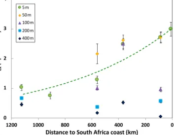
at depths below the surface mixed layer. This assumption is supported by an inspection of horizontal²²⁸Ra gradients at depths below the mixed layer (Fig. 7). Due to the sample resolution, detailed inspection is only available for the Cape Basin. Here, unlike the exponential change seen in the surface layer,²²⁸Ra_exactivities at 50 m and deeper do not show an increasing gradient towards the continental margin. This therefore argues against lateral mixing away from the shore as the major mechanism driving subsurface²²⁸Ra concentrations in the Cape Basin. In addition, the distribution of²²⁸Ra on an isopycnal surface (≈200 m depth) is largely constant and shows no lateral gradient (Fig. 7). Studies using theoret- ical models to simulate seawater²²⁸Ra distribution have also shown that the horizontal eddy mixing (K_x) has little effect on the vertical distribution of²²⁸Ra (Lamontagne and Web- ster, 2019).

The depth profiles of²²⁸Ra_exin the Argentine Basin show evidence of advective ²²⁸Ra below the mixed layer, potentially from the nearer-shore shelf waters. For example, elevated ²²⁸Ra_exvalues are seen around 400 m at Stn18 and 200 m at Stn21 (Fig. 6a and b) and these may explain the ex- tremely highK_zvalues at these stations. Although the pos-

sibility of lateral inputs cannot be entirely excluded, particularly in the Argentine Basin, the vertical variation of²²⁸Ra near the surface mixed layer still provides the first estimates of maximum vertical mixing and the upper limits of trace element inputs from vertical mixing to the surface ocean along the 40^◦S transect.

4.3 Trace element inputs in the South Atlantic

TEs are important micronutrients for marine productivity in the surface ocean. Atmospheric dust deposition is an important source of TEs to the surface ocean. The soluble atmospheric dust deposition fluxes to the surface 40^◦S At- lantic transect have been assessed from the same cruise as this study: these are 0.02–0.05 nmol Co m⁻²d⁻¹, 1.6–

5.2 nmol Fe m⁻²d⁻¹and 0.6–6 nmol Zn m⁻²d⁻¹(Chance et al., 2015). However, other inputs of these TEs to the euphotic zone in the South Atlantic are still unknown (e.g. shelf–ocean and vertical mixing). In this study, we consider three different ²²⁸Ra approaches to quantify the horizontal and vertical TE fluxes in the Cape Basin and Argentine Basin along the 40^◦S transect: (1) ²²⁸Ra-derived diffusive, (2) ²²⁸Ra- derived advective, and (3) TE/²²⁸Ra-ratio-derived TE fluxes (Sect. 2.5 and Appendix D). The results of the TE fluxes are summarised in Table 2 (shelf–ocean, horizontal) and Table 3 (vertical). For comparison, the horizontal TE fluxes are normalised to the areas of shelf–ocean cross section (Table D2;

Urien and Ewing, 1974; Nelson et al., 1998; Emery, 1966;

Windom et al., 2006; Carr and Botha, 2012; Hooker et al., 2013; Vieira et al., 2020) (illustrated in Fig. 8) unless other- wise specified.

Surprisingly, the estimates of shelf–ocean TE fluxes show relatively good agreements (within uncertainties) between these three approaches (Table 2), given the limitations of the 1-D²²⁸Ra-mixing model (Moore, 2015). A similar observation has also been found in the²²⁸Ra study in the Peruvian continental shelf (Sanial et al., 2018), which suggests that the assumptions made for the 1-D²²⁸Ra-mixing model are reasonable. In addition, the TE fluxes show consistent results between the D357 and JC068 data in the Cape Basin. These observations are likely to be a result of the gradients of²²⁸Ra and TEs representing a long-term average at an ocean basin scale and being closer to a steady-state condition in the upper water column (e.g. the²²⁸Ra and TEs in the North Atlantic;

Charette et al., 2015).

The²²⁸Ra-derived shelf–ocean Co fluxes range from 4 to 21×10³nmol m⁻²d⁻¹ in the Argentine Basin margin and from 4.3 to 6.2×10³nmol m⁻²d⁻¹in the Cape Basin margin of the 40^◦S transect in the South Atlantic. In comparison, previous studies have applied the TE/²²⁸Ra approach to estimate the shelf Co fluxes in several continental margins: the western North Atlantic (1.6×10⁵nmol m⁻²d⁻¹; Charette et al., 2016), the Peruvian shelf (1.4×10⁵nmol m⁻²d⁻¹, Sanial et al., 2018) and the Congo offshelf 3^◦S (2.8× 10⁶nmol m⁻²d⁻¹; Vieira et al., 2020). Although these fluxes

(12)

Figure 5.Plots of²²⁸Raexin the surface ocean (<10 m) along the(a)Argentine and(b)Cape Basin 40^◦S Atlantic transects, with the distributions of salinity and temperature shown in panels(c)and(d). The orange band indicates the boundary of the BrC in the Argentine Basin transect, highlighted by high salinity and temperature. The dashed red and green lines show exponential regression trends through the 228Ra_exdata (Argentine Basin transect: only to BrC; Cape Basin transect: the whole transect). The gradients of the exponential fit (thea values) are used in Eq. (3) for theKxcalculation. The errors ofaandKxare±1 SD. The dashed grey line shows a linear regression trend through the²²⁸Ra_exdata from BrC to the open ocean in the Argentine Basin transect, which is used in Eq. (4) to estimate the advection water transport velocity (w).

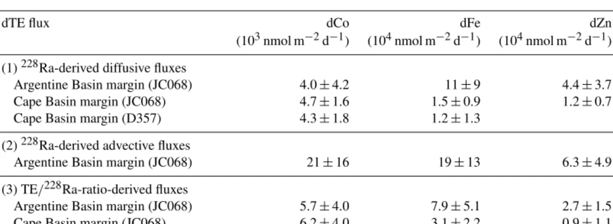
Table 2.²²⁸Ra-derived shelf–ocean dTE fluxes along the 40^◦S Atlantic transect^∗.

dTE flux dCo dFe dZn

(10³nmol m⁻²d⁻¹) (10⁴nmol m⁻²d⁻¹) (10⁴nmol m⁻²d⁻¹) (1)²²⁸Ra-derived diffusive fluxes

Argentine Basin margin (JC068) 4.0±4.2 11±9 4.4±3.7

Cape Basin margin (JC068) 4.7±1.6 1.5±0.9 1.2±0.7

Cape Basin margin (D357) 4.3±1.8 1.2±1.3

(2)²²⁸Ra-derived advective fluxes

Argentine Basin margin (JC068) 21±16 19±13 6.3±4.9

(3) TE/²²⁸Ra-ratio-derived fluxes

Argentine Basin margin (JC068) 5.7±4.0 7.9±5.1 2.7±1.5

Cape Basin margin (JC068) 6.2±4.0 3.1±2.2 0.9±1.1

∗Fluxes are normalised to the area of the cross-shelf section. All errors are±1 SD.

are about 1 and 2 orders of magnitude, respectively, higher than the estimates in the South Atlantic, these regions are also associated with low oxygen which increases dissolution of Mn and Fe oxides in sediments and is prone to result in higher Co fluxes (e.g. Hawco et al., 2016). A low shelf–ocean Co flux has been reported in the eastern South Atlantic conti-

nental shelf (11–18×10³nmol m⁻²d⁻¹; Bown et al., 2011), which is very close to this study region in the Cape Basin.

Along the 40^◦S transect, the²²⁸Ra-derived shelf–ocean Fe fluxes range from 8 to 19×10⁴nmol m⁻²d⁻¹in the Argen- tine Basin margin and from 1.2 to 3.1×10⁴nmol m⁻²d⁻¹in the Cape Basin margin, which are slightly lower than the es-

(13)

Figure 6.Depth profiles of(a–f)seawater²²⁸Ra_exactivity in red (Argentine Basin) and green (Cape Basin) circles and density (sigma-t) shown in dashed grey lines, and(g–i)density and temperature in the upper ocean shown at Stn1, 2, 3, 4.5, 18, and 21. Depths of the mixed layer are labelled with the horizontal dashed orange lines, defined by the sigma-tand temperature profiles. The dashed red and green lines show exponential regression trends through the²²⁸Raexdata below the mixed layer (including the average value of the mixed layer). The gradients of the exponential fit (theavalues) are used in Eq. (5) for theK_zcalculation (errors±1 SD).

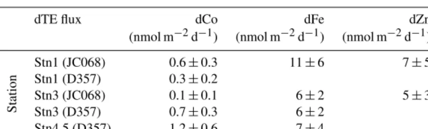
Table 3.²²⁸Ra-derived vertical dTE fluxes along the 40^◦S Atlantic transect^∗.

dTE flux dCo dFe dZn

(nmol m⁻²d⁻¹) (nmol m⁻²d⁻¹) (nmol m⁻²d⁻¹)

Station

Stn1 (JC068) 0.6±0.3 11±6 7±5

Stn1 (D357) 0.3±0.2

Stn3 (JC068) 0.1±0.1 6±2 5±3

Stn3 (D357) 0.7±0.3 6±2

Stn4.5 (D357) 1.2±0.6 7±4

∗Fluxes are normalised to the surface area. All errors are±1SD.

timates of the shelf–ocean Fe flux (4.5×10⁵nmol m⁻²d⁻¹) in the western North Atlantic (Charette et al., 2016). How- ever, these fluxes are significantly lower than those high Fe fluxes observed in regions with river plumes (e.g. Congo River; 4.1×10⁸nmol m⁻²d⁻¹; Vieira et al., 2020), submarine groundwater discharge (1.3×10⁸nmol m⁻²d⁻¹, Win- dom et al., 2006) and the oxygen minimum zone (2.1× 10⁶nmol m⁻²d⁻¹, Sanial et al., 2018).

Lastly, the ²²⁸Ra-derived shelf–ocean Zn fluxes range from 2.7 to 6.3×10⁴nmol m⁻²d⁻¹ in the Argentine and from 0.9 to 1.2×10⁴nmol m⁻²d⁻¹in the Cape Basin mar-

gins. When compared with the only available shelf–ocean Zn flux value (1.8×10⁶nmol m⁻²d⁻¹) in the western North At- lantic (Charette et al., 2016), the Zn fluxes from this study indicate low Zn inputs in the South Atlantic. The different shelf–ocean Zn inputs between the North and South Atlantic require more detailed study to understand the processes supplying and removing Zn in the shelf waters and the influence of anthropogenic Zn. Nevertheless, the low Zn inputs support the previous observation that surface water along the 40^◦S transect has some of the lowest reported dissolved Zn concentrations in the global oceans (Wyatt et al., 2014).

(14)

Figure 7.Plots of²²⁸Ra_exactivity at water depths of 5, 50, 100, 200, and 400 m versus distance to the coast of Cape Town in South Africa. The dashed line shows an exponential regression line through the data at 5 m.

From below the mixed layer, the vertical dissolved TE fluxes range from 0.1 to 1.2 nmol Co m⁻²d⁻¹, from 6 to 9 nmol Fe m⁻²d⁻¹, and from 5 to 7 nmol Zn m⁻²d⁻¹along the 40^◦S transect (Table 3). These fluxes are consistent with previous estimates of Co in the South Atlantic (0.04–

0.46 nmol m⁻²d⁻¹, Bown et al., 2011; 0.1–4 nmol m⁻²d⁻¹, Rigby et al., 2020) and in the high-latitude North Atlantic (0.15–0.5 nmol m⁻²d⁻¹, Achterberg et al., 2020), of Fe in the North Atlantic (0.14–21.1 nmol m⁻²d⁻¹; Painter et al., 2014), South Atlantic (1–27 nmol m⁻²d⁻¹; Rigby et al., 2020), and the Southern Ocean (3–31 nmol m⁻²d⁻¹, Blain et al., 2007; 2.3–14 nmol m⁻²d⁻¹, Charette et al., 2007), and of Zn in the Atlantic (2.7–137 nmol m⁻²d⁻¹, Rigby et al., 2020; Achterberg et al., 2020). However, the vertical diffusive Fe fluxes are smaller than some other vertical fluxes estimated in the Southern Ocean (27–135 nmol m⁻²d⁻¹; Du- laiova et al., 2009) and the winter mixing fluxes in the high-latitude North Atlantic (e.g. 27.3–103 nmol m⁻²d⁻¹; Achterberg et al., 2018). It is also worth mentioning that the TE fluxes estimated by Blain et al. (2007), Bown et al. (2011), and Painter et al. (2014) use theKzvalues derived from the vertical density profiles instead of²²⁸Ra.

4.4 Mass-balance budgets for trace elements in the South Atlantic

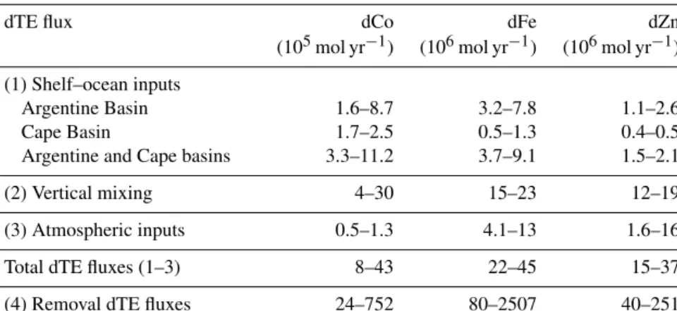
The mass-balance budgets of dissolved TEs from different sources (horizontal shelf inputs, vertical upward mixing, and atmospheric dust deposition) and sinks (exported fluxes) in the surface South Atlantic (40^◦S transect) are calculated and summarised in Table 4 and Fig. 8. The vertical upward mixing appears to be a more important source supplying TEs to the surface water at 40^◦S compared to atmospheric dust

and continental shelf inputs. However, the dominant source or seasonal variation of the vertical TE inputs cannot be identified in this study. Apart from the internal regeneration, TEs from a subsurface lateral input from the continental margin can subsequently be brought to the surface by vertical mixing (e.g. Rijkenberg et al., 2014). Deep winter convective mixing has also been shown as an important source of TEs to the surface ocean (e.g. Achterberg et al., 2018, 2020; Rigby et al., 2020).

A bulk estimate of the dissolved TE exported fluxes from the surface ocean, supported by new production biological uptake, can be made using a sinking particulate organic carbon (POC) flux and an estimated TE/C uptake ratio. In this study region, previous studies have reported the ²³⁴Th-derived POC fluxes ranging from 3.1 to 9.7 mmol C m⁻²d⁻¹ in the top 100 m integra- tion depth (7.0±2.2 mmol C m⁻²d⁻¹; Thomalla et al., 2006;

6.4±3.3 mmol C m⁻²d⁻¹; Owens et al., 2015). The estimates of cellular TE/C ratios are 0.3–3, 10–100, and 5–

10 µmol mol⁻¹ for Co/C, Fe/C, and Zn/C, respectively, based on the measurements in marine phytoplankton under different TE concentrations in surface waters (e.g. Co: 10⁻¹² to 10⁻¹¹mol L⁻¹, Sunda and Huntsman, 1995; Fe: 10⁻⁸to 10⁻⁷mol L⁻¹, Sunda and Huntsman, 1997; Zn: 10⁻¹¹ to 10⁻¹⁰mol L⁻¹, Sunda and Huntsman, 2000). These concentrations were chosen to represent the ranges of TE concentrations found in the surface waters of this region. Multiplying the POC fluxes with the TE/C ratios, the exported fluxes of Co, Fe, and Zn are 1–29, 31–970, and 16–97 nmol m⁻²d⁻¹, respectively. The results agree with the estimates of particulate TE removal fluxes in the North Atlantic (e.g. Co: 0.27–

6.8 and Fe: 274–2740 nmol m⁻²d⁻¹; Hayes et al., 2018), even though the North Atlantic assessments have accounted for both biological uptake and particle scavenging fluxes by directly using TE/²³⁴Th ratios.

In general, the exported TE fluxes are higher than the net dissolved TE inputs that we have identified in this study (Ta- ble 4). Taking Fe as an example, the total dissolved Fe inputs (22–45×10⁶mol yr⁻¹) only contribute 1 %–56 % of the biological consumption of dissolved Fe, which is not enough to balance the iron budget in the surface ocean. This could imply that (1) the spatial and temporal variability in²³⁴Th- derived POC flux is crucial (given the mean life of²³⁴Th is 35 d); (2) much lower TE/C ratios are required; or (3) other sources of TEs need to be considered (e.g. lateral-transport particulate TE or winter deep mixing).

In the calculations of TE removal fluxes, we have considered a reasonable range of²³⁴Th-derived POC fluxes and the TE/C ratios, which helps to bring the lower end of the TE removal fluxes closer to the upper end of the total TE input fluxes. This may be enough to explain the offsets of Zn and Co budgets, considering the uncertainties, but it is still not enough to explain the offset of Fe. The range of observed phytoplankton TE/C ratios in the global oceans can vary widely (e.g. Co/C: 0.00047–25.6 µmol mol⁻¹; Fe/C: 2.1–