The PMIP4 contribution to CMIP6 – Part 3: The last millennium, scientific objective, and experimental design for

(1)

https://doi.org/10.5194/gmd-10-4005-2017

The PMIP4 contribution to CMIP6 – Part 3: The last millennium, scientific objective, and experimental design for

the PMIP4 past1000 simulations

Johann H. Jungclaus¹, Edouard Bard², Mélanie Baroni², Pascale Braconnot³, Jian Cao⁴, Louise P. Chini⁵,

Tania Egorova^6,7, Michael Evans⁸, J. Fidel González-Rouco⁹, Hugues Goosse¹⁰, George C. Hurtt⁵, Fortunat Joos¹¹, Jed O. Kaplan¹², Myriam Khodri¹³, Kees Klein Goldewijk^14,15, Natalie Krivova¹⁶, Allegra N. LeGrande¹⁷,

Stephan J. Lorenz¹, Jürg Luterbacher^18,19, Wenmin Man²⁰, Amanda C. Maycock²¹, Malte Meinshausen^22,23, Anders Moberg²⁴, Raimund Muscheler²⁵, Christoph Nehrbass-Ahles¹¹, Bette I. Otto-Bliesner²⁶, Steven J. Phipps²⁷, Julia Pongratz¹, Eugene Rozanov^6,7, Gavin A. Schmidt¹⁷, Hauke Schmidt¹, Werner Schmutz⁶, Andrew Schurer²⁸, Alexander I. Shapiro¹⁶, Michael Sigl^29,30, Jason E. Smerdon³¹, Sami K. Solanki¹⁶, Claudia Timmreck¹,

Matthew Toohey³², Ilya G. Usoskin³³, Sebastian Wagner³⁴, Chi-Ju Wu¹⁶, Kok Leng Yeo¹⁶, Davide Zanchettin³⁵, Qiong Zhang²⁴, and Eduardo Zorita³⁴

1Max Planck Institut für Meteorologie, Hamburg, Germany

2CEREGE, Aix-Marseille University, CNRS, IRD, College de France, Technopole de l’Arbois, 13545 Aix-en-Provence, France

3Laboratoire des Sciences du Climat et de l’Environnement, LSCE/IPSL, CEA – CNRS-UVSQ, Université Paris-Saclay, 91191 Gif-sur-Yvette, France

4Earth System Modeling Center, Nanjing University of Information Science and Technology, Nanjing 210044, China

5Department of Geographical Sciences, University of Maryland, College Park, MD 20742, USA

6Physikalisch-Meteorologisches Observatorium Davos and World Radiation Center (PMOD/WRC), Davos, Switzerland

7Institute for Atmospheric and Climate Science, ETH Zurich, Zurich, Switzerland

8Dept. of Geology and Earth System Science Interdisciplinary Center, University of Maryland, College Park, MD 20742, USA

9Dept. of Astrophysics and Atmospheric Sciences, IGEO (UCM-CSIC), Universidad Complutense de Madrid, 28040 Madrid, Spain

10ELI/TECLIM, Université Catholique de Louvain, Louvain-la-Neuve, Belgium

11Climate and Environmental Physics, Physics Institute and Oeschger Centre for Climate Change Research, University of Bern, Bern, Switzerland

12Institute of Earth Surface Dynamics, University of Lausanne, Lausanne, Switzerland

13Laboratoire d’Océanographie et du Climate, Sorbonne Universités, UPMC Université Paris 06, IPSL, UMR CNRS/IRD/MNHN, 75005 Paris, France

14Copernicus Institute of Sustainable Development, Utrecht University, Utrecht, the Netherlands

15PBL Netherlands Environmental Assessment Agency, The Hague/Bilthoven, the Netherlands

16Max-Planck-Institut für Sonnensystemforschung, Göttingen, Germany

17NASA Goddard Institute for Space Studies, 2880 Broadway, New York, USA

18Department of Geography, Climatology, Climate Dynamics and Climate Change, Justus Liebig University Giessen, Giessen, Germany

19Centre for International Development and Environmental Research, Justus Liebig University Giessen, Giessen, Germany

20LASG Institute of Atmospheric Physics, Chinese Academy of Sciences, Beijing, China

21School of Earth and Environment, University of Leeds, Leeds, UK

22Australian-German Climate & Energy College, the University of Melbourne, Australia

23Potsdam Institute for Climate Impact Research, Potsdam, Germany

(2)

24Department of Physical Geography and Bolin Centre for Climate Research, Stockholm University, Stockholm, Sweden

25Department of Geology, Lund University, Lund, Sweden

26National Center for Atmospheric Research, Boulder, Colorado 80305, USA

27Institute for Marine and Antarctic Studies, University of Tasmania, Hobart, Tasmania, Australia

28GeoSciences, University of Edinburgh, Edinburgh, UK

29Laboratory of Environmental Chemistry, Paul Scherrer Institute, 5232 Villigen, Switzerland

30Oeschger Centre for Climate Change Research, University of Bern, 3012 Bern, Switzerland

31Lamont-Doherty Earth Observatory of Columbia University, Palisades, NY, USA

32GEOMAR Helmholtz Centre for Ocean Research Kiel, Kiel, Germany

33Space Climate Research Group and Sodankylä Geophysical Observatory, University of Oulu, Oulu, Finland

34Institute for Coastal Research, Helmholtz-Zentrum Geesthacht, Geesthacht, Germany

35Department of Environmental Sciences, Informatics and Statistics, University of Venice, Mestre, Italy Correspondence to:Johann H. Jungclaus (johann.jungclaus@mpimet.mpg.de)

Received: 3 November 2016 – Discussion started: 24 November 2016

Revised: 5 July 2017 – Accepted: 14 July 2017 – Published: 7 November 2017

Abstract. The pre-industrial millennium is among the periods selected by the Paleoclimate Model Intercompari- son Project (PMIP) for experiments contributing to the sixth phase of the Coupled Model Intercomparison Project (CMIP6) and the fourth phase of the PMIP (PMIP4). The past1000 transient simulations serve to investigate the response to (mainly) natural forcing under background conditions not too different from today, and to discriminate between forced and internally generated variability on interan- nual to centennial timescales. This paper describes the mo- tivation and the experimental set-ups for the PMIP4-CMIP6 past1000 simulations, and discusses the forcing agents orbital, solar, volcanic, and land use/land cover changes, and variations in greenhouse gas concentrations. The past1000 simulations covering the pre-industrial millennium from 850 Common Era (CE) to 1849 CE have to be complemented by historical simulations (1850 to 2014 CE) following the CMIP6 protocol. The external forcings for thepast1000ex- periments have been adapted to provide a seamless transition across these time periods. Protocols for thepast1000simu- lations have been divided into three tiers. A default forcing data set has been defined for the Tier 1 (the CMIP6past1000) experiment. However, the PMIP community has maintained the flexibility to conduct coordinated sensitivity experiments to explore uncertainty in forcing reconstructions as well as parameter uncertainty in dedicated Tier 2 simulations. Addi- tional experiments (Tier 3) are defined to foster collaborative model experiments focusing on the early instrumental period and to extend the temporal range and the scope of the simulations. This paper outlines current and future research foci and common analyses for collaborative work between the PMIP and the observational communities (reconstructions, instrumental data).

1 Introduction

Based on a vast collection of proxy and observational data sets, the Common Era (CE; approximately the last 2000 years) is the best-documented interval of decadal- to centennial-scale climate change in Earth’s history (PAGES2K Consortium, 2013; Masson-Delmotte et al., 2013). Climate variations during this period have left their traces on human history, such as the documented impacts of the Medieval Climate Anomaly (MCA) and the Little Ice Age (LIA) (e.g. Pfister and Brázdil, 2006; Büntgen et al., 2016; Xoplaki et al., 2016; Camenisch et al., 2016). Nev- ertheless, there is still a debate regarding the relative contribution of internal variability and external forcing factors to natural fluctuations in the Earth’s climate system and how they compare to the present anthropogenic global warming (Masson-Delmotte et al., 2013). This is particularly acute for regional and sub-continental scales, where spatially hetero- geneous variability modes potentially impact the climate signal (e.g. PAGES2k-PMIP3 Group, 2015; Luterbacher et al., 2016; Gagen et al., 2016). Simulations covering the recent past can thus provide context for the evolution of the modern climate system and for the expected changes during the coming decades and centuries. Furthermore, they can help to identify plausible mechanisms underlying palaeoclimatic observations and reconstructions. Here, we describe and dis- cuss the forcing boundary conditions and experimental protocol for thepast1000simulations covering the pre-industrial millennium (850 to 1849 CE) as part of the fourth phase of the Paleoclimate Model Intercomparison Project (PMIP4, Kageyama et al., 2016) and the sixth phase of the Coupled Model Intercomparison Project (CMIP6, Eyring et al., 2016).

We emphasise that thepast1000simulations must be complemented byhistoricalsimulations for 1850 to 2014 CE fol-

(3)

lowing the CMIP6 protocol and applying the CMIP6 external forcing for the industrial period (Eyring et al., 2016, and references therein).

Simulations of the CE have applied models of varying complexity. Crowley (2000) and Hegerl et al. (2006) used energy balance models to study the surface temperature response to changes in external forcing, particularly solar, volcanic, and greenhouse gas concentrations (GHG). Earth system models (ESMs) of intermediate complexity (e.g. Goosse et al., 2005) have been used to perform long integrations or multiple (ensemble) simulations requiring relatively small amounts of computer resources. Finally, coupled atmosphere ocean general circulation models (AOGCMs) and comprehensive ESMs have enabled the community to gain further insights into internally generated and externally forced variability, investigating climate dynamics, modes of variability (e.g. González-Rouco et al., 2003; Raible et al., 2014; Ortega et al., 2015; Zanchettin et al., 2015; Landrum et al., 2013), and regional processes in greater detail (Goosse et al., 2006, 2012; PAGES2k-PMIP3 Group, 2015; Coats et al., 2015;

Luterbacher et al., 2016). They have also allowed individual groups to study specific components of the climate system, such as the carbon cycle (Jungclaus et al., 2010; Lehner et al., 2015; Chikamoto et al., 2016), or aerosols and short-lived gases (e.g. Stoffel et al., 2015). Recent increases in com- puting power have made it feasible to carry out millennial- scale ensemble simulations with comprehensive ESMs (e.g.

Jungclaus et al., 2010; Otto-Bliesner et al., 2016). Ensemble approaches are extremely beneficial as a means of separat- ing and quantifying simulated internal variability and the responses to changes in external forcing, under the assumption that the simulation variance within the ensemble is a reason- able estimate of the unforced variability of the actual climate system (e.g. Deser et al., 2012; Stevenson et al., 2016).

The past1000experiment was adopted as a standard experiment in the third phase of PMIP (PMIP3, Braconnot et al., 2012), which was partly embedded within the fifth phase of CMIP (CMIP5, Taylor et al., 2012). This was an important step as it encouraged modelling groups to use the same climate models for future scenarios and for palaeoclimate simulations, instead of stripped-down or low-resolution versions.

Using the same state-of-the-art ESMs to simulate both past and future climates allows palaeoclimate data to be used to evaluate the same models that are, in turn, employed to gen- erate future climate projections (Schmidt et al., 2014). The PMIP3past1000experiments were based on a common protocol describing a variety of suitable forcing boundary conditions (Schmidt et al., 2011, 2012). Moreover, a common structure of the CMIP5 output facilitated multi-model analyses, comparisons with reconstructions, and connections to future projections (e.g. Bothe et al., 2013; Smerdon et al., 2015; PAGES2k-PMIP3 Group, 2015; Cook et al., 2015).

Several studies have also addressed variations and responses of the carbon cycle (e.g. Brovkin et al., 2010; Lehner et al., 2015; Keller et al., 2015; Chikamoto et al., 2016). Last-

millennium-related contributions to several chapters of As- sessment Report 5 of the Intergovernmental Panel on Climate Change (IPCC-AR5) (Masson-Delmotte et al., 2013; Flato et al., 2013; Bindoff et al., 2013) highlighted the value of the past1000multi-model ensemble.

Further progress is expected for CMIP6 and PMIP4. Mod- els with higher spatial resolution will be available for long- term palaeo simulations, which has the potential to improve the representation of mechanisms controlling regional variability and to alleviate biases in the mean state (e.g. Milin- ski et al., 2016). Newly added model components, for example interactive chemistry and aerosol microphysics, will allow for more explicit representation of forcing-related processes in some models (e.g. LeGrande et al., 2016), and, as we outline below, improvements in forcing reconstructions regarding their accuracy and complexity will potentially lead to improved quality in comparative model–data studies. In addition, more stringent protocols for experimental set-ups (e.g. an identical forcing data set for the Tier 1 experiment) and output data are implemented in the CMIP6 process, providing an improved basis for multi-model studies. The CMIP6 protocols also ensure a better interaction between related MIPs. For example, the PMIP4past1000ex- periment is closely related to the more process-oriented suite of simulations in the Model Intercomparison Project on the climatic response to volcanic forcing (VolMIP, Zanchettin et al., 2016).

The PMIP working group on the climate evolution over the last 2000 years (WG Past2K) is closely cooperating with the PAGES (Past Global Changes) 2k Network pro- moting regional reconstructions of climate variables and modes of variability. Collaborative work has focused on reconstruction–model intercomparison (e.g. Bothe et al., 2013; Moberg et al., 2015; PAGES2k-PMIP3 Group, 2015) and assessment of modes of variability (e.g. Raible et al., 2014). Integrated assessment of reconstructions and simulations has led to progress in model evaluation and process un- derstanding (e.g. Lehner et al., 2013; Sicre et al., 2013; Jung- claus et al., 2014; Man et al., 2012; Man and Zhou, 2014).

The increasing number of available simulations and reconstructions has also created a need for development of new statistical modelling approaches dedicated to model–data comparison analysis (e.g. Sundberg et al., 2012; Barboza et al., 2014; Tingley et al., 2015; Bothe et al., 2013). The combination of real-world proxies with simulated “pseudo” proxies has improved the interpretation of the reconstructions (e.g.

Smerdon, 2012) and helped to provide information for the selection of proxy sites and numbers (Wang et al., 2014;

Zanchettin et al., 2015; Smerdon et al., 2015; Hind et al., 2012; Lehner et al., 2012; Ortega et al., 2015). Despite significant advances in our ability to simulate reconstructed past changes, challenges still remain, for example, regarding hy- droclimatic changes in the last millennium (Anchukaitis et al., 2010; Ljungqvist et al., 2016). Documenting progress and the status of achievements and challenges in the multi-model

(4)

context is a major goal of PMIP as the community embarks on a new round of model intercomparison projects.

This paper is part of a suite of five documenting the PMIP contributions to CMIP6. Kageyama et al. (2016) provide an overview of the five selected time periods and the experiments. More specific information is given in the contributions for the mid-Holocene (midHolocene) and the previous interglacial (lig127k) by Otto-Bliesner et al. (2017), for the last glacial maximum (lgm) by Kageyama et al. (2017), and for the mid-Pliocene warm period (midPliocene) by Hay- wood et al. (2016), and the present paper on the last millennium (past1000). PMIP has adopted the CMIP6 categori- sation where the highest-priority experiments are classified as Tier 1, whereas additional sensitivity experiments or dedicated studies are Tier 2 or Tier 3. The standard experiments for the five periods are all ranked Tier 1. Modelling groups are not obliged to run all PMIP4-CMIP6 experiments. It is mandatory, however, for all participating groups to run at least one of the experiments that were run in previous phases of PMIP (i.e.midHoloceneorlgm).

Our past1000paper is organised as follows. In Sect. 2, we review the major forcing agents for climate evolution during the CE in the light of previous simulations of the past. Section 3 describes the experimental protocols for the Tier 1 to Tier 3 categorised experiments. Section 4 describes the derivations and the characteristics of the forcing boundary conditions. Section 5 discusses the relations between the PMIP experiments and the overarching research questions of CMIP6 and links to other MIPs. Section 6 provides a con- cluding discussion.

2 Drivers of climate variations during the CE

The major forcing agents during the pre-industrial millennium are changes in orbital parameters, solar irradiance, stratospheric aerosols of volcanic origin, and greenhouse gas (GHG) concentrations. Additional anthropogenic impacts arise from aerosol emissions and changes in land surface properties as a result of land use (e.g. Pongratz et al., 2009; Kaplan et al., 2011). External drivers affect the climate system in several ways, ranging from millennial-scale trends, such as those induced by changing orbital parameters, to the response of relatively short-lived disturbances of the radiative balance, as in the case of volcanic activity. Ad- ditionally, feedbacks internal to the climate system may am- plify, delay, or prolong the effect of forcing (e.g. Shindell et al., 2001; Swingedouw et al., 2011; Zanchettin et al., 2012).

The PMIP4 experiments will revisit the questions regarding the relative role of external drivers using updated forcing data sets and a new generation of climate models, in which the different forcing will be better represented. The increase in model resolution and the additional implementations in the number of Earth system components for most ESMs will pro-

vide more realistic simulation and assessment of the impact of external forcings for sub-continental climate changes.

Volcanic eruptions are among the most prominent drivers of natural climate variability. Reconstructions for the CE show clear relationships between well-documented eruptions and climate impacts, for example the April 1815 CE Mount Tambora eruption and the subsequent “year without a sum- mer” (Stommel and Stommel, 1983; Raible et al., 2016, for a review). In addition to short-lived effects on the radiative balance, volcanic events can have long-lasting effects. Clus- ters of eruptions have been proposed as the major contribution for the transition from the MCA to the LIA (Miller et al., 2012; Lehner et al., 2013), and for the long-term global cooling trend during the pre-industrial CE (McGregor et al., 2015).

Whereas model simulations generally reproduce the sum- mer cooling, as well as aspects of regional and delayed responses to volcanic eruptions (Zanchettin et al., 2012, 2013;

Atwood et al., 2016), there are discrepancies between model results and the observed climate evolution, in particular regarding the amplitude of the response to volcanic eruptions (e.g. Brohan et al., 2012; Evans et al., 2013; Wilson et al., 2016; Anchukaitis et al., 2010). Possible reasons for this disagreement include shortcomings in the volcanic reconstructions used to drive the models, or in the realism of the implementation of the aerosol forcing in the model schemes, deficiencies in reproducing the dynamic responses in the atmosphere and ocean (e.g. Charlton-Perez et al., 2013;

Ding et al., 2014), or sampling biases (Anchukaitis et al., 2012; Lehner et al., 2016). The recent review by Kremser et al. (2016) concluded that the uncertainty arising from calibration of the aerosol properties to the observational period propagates into the estimated magnitude of the inferred responses in the stratospheric aerosol reconstructions. Tak- ing into account non-linear aerosol microphysics processes for the calculation of the volcanic aerosol radiative forcing (RF) has improved the compatibility between reconstructed and simulated climate (Timmreck et al., 2009; Stoffel et al., 2015). However, differences in the complexity and technical implementation of aerosol microphysics can lead to consid- erable differences in the resulting RF, even when the same sulfur dioxide injections are prescribed (Timmreck, 2012;

Zanchettin et al., 2016).

Solar irradiance changes can be a significant forcing factor on decadal to centennial timescales (Gray et al., 2010).

The generally cooler conditions during the LIA have often been attributed to the co-occurring grand minima, such as the Maunder Minimum (1645–1715 CE; Eddy, 1976) that was characterised by an almost total absence of sunspots.

However, attribution studies indicate that reduced solar forcing had a smaller impact on surface temperatures during the LIA compared to contemporary volcanic activity (Hegerl et al., 2011; Schurer et al., 2013, 2014; see also Bindoff et al., 2013).

(5)

Prior to PMIP3-CMIP5, simulations of the last millennium used solar reconstructions with a relatively broad range of total solar irradiance (TSI) variations (0.05–0.29 %) as characterised by the change from the Late Maunder Min- imum (ca. 1675–1715 CE, Luterbacher et al., 2001; LMM hereafter) to the late 20th century (1960 to 1990 CE, e.g.

Ammann et al., 2007; Fernández-Donado, 2015). Note that a 0.25 % change is equivalent to a variation of about 3.4 W m⁻²in TSI. However, the higher TSI changes since the LMM, provided mostly by earlier calibrations based on the analysis of data from Sun-like stars (Baliunas et al., 1995), were found to be unjustifiable in the light of re-analysis of stellar data by Hall and Lockwood (2004) and Wright (2004) (see also the review by Solanki et al., 2013). Therefore, the revised solar forcing reconstructions presented in Schmidt et al. (2011) exhibit typical LMM-to-present changes of 0.04 to 0.1 %. Based on independent alternative assumptions for the calibration of grand solar maxima, Shapiro et al. (2011) derived a solar forcing reconstruction that exhibited a much larger long-term modulation (∼0.44 %) than any other. This data set was included in the update of the PMIP3past1000 protocol by Schmidt et al. (2012). Later assessment of the Shapiro et al. (2011) reconstruction (Judge et al., 2012, and references therein) indicated, however, that its large amplitude is likely an overestimation (see below).

Because reconstructions of past solar forcing tend to cluster in simulations using either relatively high (i.e. mostly pre- PMIP3) or low (PMIP3) estimates of solar variations, several studies have investigated which of these provide a better fit to temperature reconstructions, but the results have so far been mixed. Whereas simulations with larger TSI variability give a somewhat better representation of the size of the MCA–LIA transition for Northern Hemisphere temperatures (Fernández-Donado et al., 2013), statistical assessment (Hind and Moberg, 2013; Moberg et al., 2015;

PAGES2k-PMIP3 group, 2015) and more detailed regional analyses (e.g. Luterbacher et al., 2016) were inconclusive.

The significantly higher-amplitude reconstruction by Shapiro et al. (2011) was used in a climate model of intermediate complexity (Feulner, 2011), the HadCM3 climate model (Schurer et al., 2014), and the SOCOL model (Anet et al., 2014). Whereas the first two studies reported a climate response incompatible with reconstructions, Anet et al. (2014) argued that high-amplitude forcing variations were necessary in their model to reproduce the cooling during the Dalton Minimum.

One of the major anthropogenic influences on the climate system over the past 2000 years was land cover change as a result of conversion of natural vegetation, mainly to agricultural and pastoral uses. The climatic effects of anthropogenic land cover change (ALCC) are undisputed in the modern world, and it is increasingly recognised that land use in the late pre-industrial Holocene may have also had substantial effects on climate. In parts of the world where ALCC led to quasi-permanent deforestation and where climate is tightly

coupled to land surface conditions, we might expect regional climate to have been strongly influenced by biogeophysical feedbacks (e.g. Cook et al., 2012; Dermody et al., 2012; Pon- gratz et al., 2009; Strandberg et al., 2014). Additionally, permanent deforestation and loss of soil carbon as a result of cultivation (e.g. Kaplan et al., 2011; Pongratz et al., 2009) may have been substantial enough to affect global climate through the biogeochemical feedback of CO₂emissions to the atmosphere (Ruddiman et al., 2016). These effects are, however, controversial (Kaplan, 2015; Nevle et al., 2011; Pongratz et al., 2012; Stocker et al., 2014).

3 The experiments

PMIP discriminates between the experiments that are en- dorsed by the World Climate Research Program (WCRP) CMIP6 committee (PMIP4 Tier 1:past1000,Mid Holocene and Last Interglacial, Last Glacial Maximum, and Mid Pliocene Warm Period; see Kageyama et al., 2016) and additional simulations (PMIP4 Tier 2 and Tier 3) that are more tailored to specific interests of the palaeoclimate modelling community. This distinction is motivated by the PMIP3 ex- perience that only a limited number of participating groups were able to afford computational resources for multiple multi-centennial simulations. In contrast to the PMIP3 protocol, PMIP4-CMIP6 recommends a single collection of external forcing data sets (the default forcing) in the Tier 1 experiments while encouraging exploration of forcing uncertainty as part of dedicated Tier 2 experiments. These Tier 2 experiments only differ in their characteristics and combination of the external drivers from the Tier 1past1000experiment.

The additional Tier 3 experiments are designed to allow clusters of modelling groups to perform dedicated research by exploring either specific episodes or extending them beyond the 1st millennium AD back in time. An overview of the experiments is given in Table 1.

The PMIP4-CMIP6 past1000 simulations will build on the CMIP6 Diagnostic, Evaluation, and Characterization of Klima (DECK) experiments (Eyring et al., 2016), in particular the “pre-industrial” control (piControl) simulation as a reference with non-varying forcing reflecting the boundary conditions at 1850 CE. Thepast1000simulations are closely related to the CMIP6historical (1850 to 2014 CE) simulations, for which they may provide more appropriate initial conditions than unforcedpiControlruns. It is expected that a number of modelling groups will be able to deliver multiple realisations of the standardpast1000experiment.

The model versions used to carry out PMIP4-CMIP6 simulations have to be the same as those documented by the respective CMIP6 DECK and historical simulations. It is mandatory to complement the transientpast1000andpast2k simulations with historical experiments following the respective CMIP6 protocol (Eyring et al., 2016).

(6)

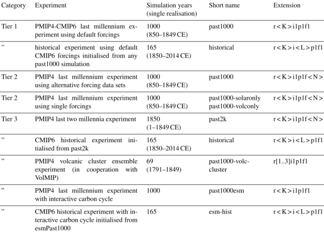
Table 1.List of experiments. In the right column the extension defines the ensemble member by the quad K, L, M, and N of integer indices for

“realisation” (r), “initialisation” (i), “perturbed physics” (p), and “forcing (f). Modelling groups need to document the choices, in particular for initialisation and forcing. Note that “f1” should be reserved for the default PMIP4-CMIP6 forcing.

Category Experiment Simulation years

(single realisation)

Short name Extension

Tier 1 PMIP4-CMIP6 last millennium experiment using default forcings

1000

(850–1849 CE)

past1000 r < K > i1p1f1

” historical experiment using default CMIP6 forcings initialised from any past1000 simulation

165

(1850–2014 CE)

historical r < K > i < L > p1f1

Tier 2 PMIP4 last millennium experiment using alternative forcing data sets

1000

(850–1849 CE)

past1000 r < K > i1p1f < N >

Tier 2 PMIP4 last millennium experiment using single forcings

1000

(850–1849 CE)

past1000-solaronly past1000-volconly

r < K > i1p1f < N >

Tier 3 PMIP4 last two millennia experiment 1850 (1–1849 CE)

past2k r < K > i1p1f < N >

” CMIP6 historical experiment initialised from past2k

165

(1850–2014 CE)

historical r < K > i < L > p1f1

” PMIP4 volcanic cluster ensemble experiment (in cooperation with VolMIP)

69

(1791–1849)

past1000-volc- cluster

r[1..3]i1p1f1

” PMIP4 last millennium experiment with interactive carbon cycle

1000 past1000esm r < K > i1p1f1

” CMIP6 historical experiment with interactive carbon cycle initialised from esmPast1000

165 esm-hist r < K > i < L > p1f1

3.1 Initial state

The pre-industrial millennium is defined as covering the period 850 to 1849 CE. With the exception of PMIP4 experiment “past2K” and VolMIP-related experiment “past1000- volc-cluster” (see below), all past1000simulations start in 850 CE. As in PMIP3, this date was chosen in order to start the simulations significantly earlier than the MCA, which occurred at the beginning of the last millennium (ca. 950–

1250 CE). Another reason is that the mid-to-late 9th century CE is estimated to have been a relatively quiet period in terms of external forcing variations or occurrence of volcanic events (e.g. Sigl et al., 2015; Bradley et al., 2016).

To provide initial conditions for the simulations, it is recommended that a spin-up simulation is performed, depart- ing from the CMIP6piControlexperiment, with all forcing parameters set to ∼850 CE values. The length of this spin- up simulation will be model- and resource-dependent. How- ever, it should be long enough to minimise at least surface climate trends (Gregory, 2010). The spin-up has to be documented and this should include information on a few key variables (see Sect. 3.6). The spin-up should be consistent with the piControl (for example, it should include a back-

ground volcanic aerosol level and appropriate anthropogenic modifications to land use/land cover characteristics (as for thepiControlsimulation; see Eyring et al., 2016).

3.2 PMIP4-CMIP6 Tier 1: the standard

PMIP4-CMIP6past1000simulation plus the CMIP6historicalsimulation

The standard PMIP4-CMIP6 past1000 experiment applies the default forcing data set (see below) and is complemented by ahistorical(1850–2014 CE) simulation that uses the end state of thepast1000simulation in 1850 CE for initialisation and that follows the CMIP6 protocol (Eyring et al., 2016).

This procedure provides a consistent data set for past and present climate variations. Comparing historical simulations initialised from a piControl run (the CMIP6 default) with those starting from 1849 CE conditions frompast1000serves to assess the impact of initial conditions on the evolution of the 19th and 20th century climate.

Modelling groups are encouraged to extend this set of experiments to multiple realisations, using the same forcing but with perturbed initial conditions. While an ensemble size of 10 has been shown to be desirable (Otto-Bliesner et al., 2016;

(7)

Stevenson et al., 2016), we acknowledge that limitations in computational resources or high computational demand of high-resolution models may prevent groups from producing large ensembles.

3.3 PMIP4 Tier 2: forcing uncertainty and attribution The Tier 2 category experiments are recommended to further explore uncertainties related to external drivers. Without tak- ing uncertainties in forcing into account, model–observation discrepancies might be wrongly attributed to model failures and/or systematic problems in proxy reconstructions. The Tier 2past1000experiments should be set up in a similar way to the Tier 1past1000experiment, i.e. the simulation should cover the period 850 to 1849 CE and the same initial conditions should be used. As for Tier 1, there should be ahistori- calsimulation complementing each Tier 2past1000simula- tion. For experiment naming and identification, see Table 1.

3.3.1 Alternative forcings

Uncertainties in the reconstruction of forcing agents are associated with the source data (mostly proxies), reconstruction methodology, calibration to records representing present conditions, or the way that the forcing time series are deduced from more explicit modelling approaches. PMIP4 provides forcing data sets derived through different methodolo- gies (e.g. for solar irradiance; see below) as well as different versions of the same forcing data set (e.g. by varying parameters in the construction scheme). It also promotes the assessment of independently derived reconstructions that will be- come available during the evolution of PMIP4. For example, modelling groups are encouraged to explore and document the impact on simulated climate resulting from variations in volcanic forcing associated with the uncertainty in the trans- lation from sulfur injections to aerosol optical properties.

3.3.2 Individual forcing agents

The role of individual drivers can be assessed by perform- ing single-forcing simulations (e.g. Pongratz et al., 2009;

Schurer et al., 2014; Otto-Bliesner et al., 2016). However, low signal-to-noise ratios and the dependence of the response to varying background conditions (Zanchettin et al., 2013) require careful analyses and will be most beneficial if performed in ensemble mode (Schurer et al., 2014; Otto- Bliesner et al., 2016).

3.4 PMIP4 Tier-3: additional experiments

The Tier 3 category experiments will enable clusters of modelling groups to perform dedicated research by either exploring specific episodes or advancing the scope of thepast1000 simulations. For experiment naming and identification, see Table 1.

3.4.1 Volcanic forcing and climate change in the early instrumental period: thepast1000-volc-cluster Because many groups will not be able to perform ensemble simulations over the entire period, we suggest perform- ing multiple realisations of the early 19th century. This period is characterised by relatively strong variations in solar activity, including the Dalton Minimum, and strong volcanic eruptions in 1809, 1815, and 1835 CE. It is the coldest period of the past 500 years, and it is well documented as part of the early instrumental period (e.g. Brohan et al., 2012).

The experiment will be carried out in cooperation with the Model Intercomparison Project on the climatic response to volcanic forcing (VolMIP, Zanchettin et al., 2016). The experiment requires an ensemble (minimum three members) of 70-year long simulations starting frompast1000restart files in 1790 CE. In contrast to VolMIP experiment “volc-cluster- mill”, all external drivers remain active.

3.4.2 Thepast2Kexperiment

With the advent of longer reconstructions, in particular for volcanic eruptions (e.g. Sigl et al., 2015; Toohey and Sigl, 2017), it is now possible to start the simulations at the beginning of the 1st millennium CE. In fact, except for the land use change forcing, all forcing reconstructions described above for the Tier 1past1000experiment are available for the entire CE, and the groups need to make sure that the same forcing is used forpast1000andpast2kduring the period 850 to 1849 CE. Additional forcing reconstructions (e.g. land use) will be completed during the course of PMIP4. Thepast2k simulations will provide a basis for the analyses of specific periods in the 1st millennium CE that have attracted attention based on historical evidence, for instance, those related to the Roman Empire (Büntgen et al., 2011; Luterbacher et al., 2016) and to the onset and evolution of the “Late An- tique Little Ice Age” (Büntgen et al., 2016; Toohey et al., 2016a). Additionally, there is a growing archive of lower- resolution syntheses of marine sediment-based reconstructions that span the full CE (Marcott et al., 2013; McGregor et al., 2015). Thepast2Kexperiment will allow the community to better investigate the full span of the Medieval period and its temporal evolution, as the start of thepast1000ex- periment in the year 850 CE might neglect some important initial conditions constrained during preceding periods (see also Bradley et al., 2016). Prior to the start of the experiment, a spin-up procedure similar to thepast1000experiment has to be undertaken for year 1 CE conditions.

3.4.3 Including an interactive carbon cycle: the past1000esmexperiment

PMIP4 will extend the scope of thepast1000experiment and include simulations with models that include an interactive carbon cycle. Complementing the esm-piControland esm-

(8)

histexperiments performed by the Coupled Climate Carbon Cycle Modelling Intercomparison Project (C4MIP; Jones et al., 2016), carbon cycle feedbacks, and interaction will be studied in the pre-industrial millennium.

3.5 Experiment identification

The experiments are defined by their short name (e.g.

past1000) and an extension following the “ripf” classifica- tion, where “r” stands for “realisation, “i” for initialisation,

“p” for perturbed physics, and “f” for forcing (Table 1). The letters r, i, p, and f are followed by integers K, L, M, and N, respectively. For example, different realisations within an ensemble would have different values for “K” following the “r”.

To classify a simulation with a model with modified physical parameterisation, one would vary the integer “M” after the

“p”. The experiments using the default forcing are defined by “f1”; alternative or single forcing would be identified by a different integer value “N”. CMIP6historicalsimulations starting from apast1000run should vary the integer “L” after the “i”.

3.6 Documenting the simulations

The modelling groups are responsible for a comprehensive documentation of the model system and the experiments. A PMIP4 special issue in GMD and Climate of the Past has been opened where the groups are encouraged to publish these documentations. The documentation should include the following.

– The model version and specifications, like interactive vegetation or interactive aerosol modules

– A link to the DECK experiments performed with this model version

– Specification of the forcing data sets used and their implementation in the model

– A documentation of the spin-up strategy to arrive at 850 CE (1 CE for past2k) initial conditions. We request information on drift in key variables for a few hundred years at the end of the spin-up and the beginning of the actual experiment. These variables are

– globally and annually averaged SSTs;

– deep ocean temperatures (global and annual average over depths below 2500 m);

– deep ocean salinity (global and annual average over depths below 2500 m);

– top of atmosphere energy budget (global and annual average);

– surface energy budget (global and annual average);

– northern sea ice (annual average over the Northern Hemisphere);

– southern sea ice (annual average over the Southern Hemisphere);

– northern surface air temperature (annual average over the Northern Hemisphere);

– southern surface air temperature (annual average over the Southern Hemisphere);

– the Atlantic Meridional Overturning Circulation (maximum overturning in the North Atlantic basin); and

– the carbon budget by the biosphere.

3.7 Output variables and data distribution

The Tier 1 past1000 simulation is part of the CMIP6 experiment family and output data will be distributed through the official CMIP6 channels via the Earth System Grid Federation (ESGF, https://earthsystemcog.org/projects/wip/

CMIP6DataRequest).

Data from PMIP4-only Tier 2 and Tier 3 simulations must be processed following the same standards for data process- ing (e.g. CMOR standards) and should be distributed via ESGF.

Groups contributing past1000 simulations to CMIP6- PMIP4 should ideally deliver the entire set defined in the data request. However, an important issue for long-term simulations such as past1000is storage demand for high- frequency output. As a minimum, we ask for a subset of two- dimensional daily variables that allow investigations into extreme events and particular dynamical features, including near surface air temperature (tas), daily maximum near surface air temperature (tasmax), daily minimum near surface air temperature (tasmin), daily maximum near-surface wind speed (sfcWindmax), precipitation (pr), sea-level pres- sure (mslp), 500 hPa geopotential (zg500), and daily maximum hourly precipitation rate (prhmax). If storage of high- frequency output for the entire millennium should be too demanding, we recommend concentrating efforts on three multi-decadal periods (in descending priority): (1) the early 19th century (1790 to 1849 CE as the focus period of VolMIP), and (2) the Maunder Minimum (1645 to 1715 CE), and (3) the Medieval Climate Anomaly (1100 to 1170 CE) covering periods of high and low solar activity, respectively.

Groups participating in PMIP and VolMIP should pay attention to the new diagnostics of volcanic instantaneous radiative forcing defined by VolMIP, whose calculation is recommended for some major volcanic events simulated in the past1000experiment (for details, see Zanchettin et al., 2016).

Groups that run the PMIP4-CMIP6 experiments with the carbon cycle enabled should pay attention to the output variables requested by OCMIP and C4MIP.

The list of variables requested by PMIP for the PMIP4- CMIP6 palaeoclimate experiments can be found here: http:

//clipc-services.ceda.ac.uk/dreq/u/PMIP.html. This request is presently processed by the CMIP6 Working Group

(9)

for Coupled Modeling Infrastructure Panel (WIP) into tables, which define the variables included in the data request to the modelling groups for data to be con- tributed to the archive. The most up-to-date list including all variables requested for CMIP6 can be found at the WIP site: http://proj.badc.rl.ac.uk/svn/exarch/CMIP6dreq/

tags/latest/dreqPy/docs/CMIP6_MIP_tables.xlsx.

The last two columns in each row list MIPs associated with each variable. The first column in this pair lists the MIPs, which are requesting the variable in one or more experiments. The second column lists the MIPs proposing experiments in which this variable is requested.

As the Supplement to this paper we provide version 1.00.12 (June 2017) of the table. We note, however, that this document is still in development and inconsistencies may still exist.

4 Description of forcing boundary conditions

Some of the forcing fields are extensions in time of the “official” CMIP6 data sets for thehistoricalsimulations. These are documented in individual contributions to the GMD special issue on CMIP6 and available through the contributors’

web sites (see below and Appendices). PMIP4 specific time series and reconstructions are available via the PMIP4 web- site and specifications on data format and technical implementation are given in the Appendices.

4.1 Orbital forcing

Over the pre-industrial millennium, the orbital forcing is dominated by changes in the perihelion, whereas variations in eccentricity and obliquity are rather small (Berger, 1978;

see also Fig. 1 in Schmidt et al., 2011). The orbital forcing remains unchanged from what was used in PMIP3 (Schmidt et al., 2011). Note, however, that the reference insolation year is 1860 CE in CMIP6 (Eyring et al., 2016), compared to 1950 in PMIP3. Unless the models calculate the orbital parameters internally, groups will use a list of annually varying orbital parameters (eccentricity, obliquity, and perihelion longitude), changing every 1 January (see Appendix A1).

4.2 Greenhouse gas forcing

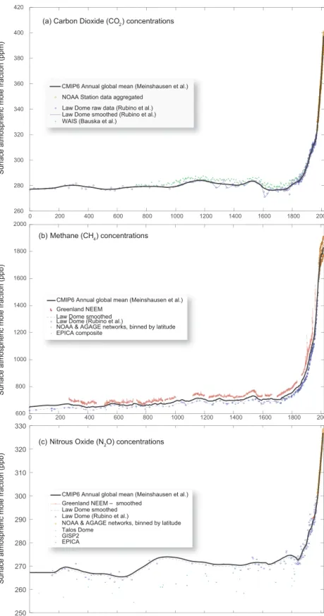
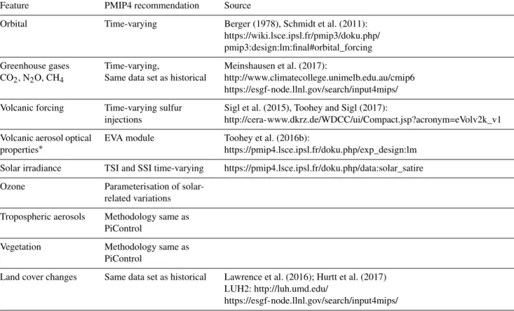
GHG time series for concentration-driven simulations are provided by CMIP6 for the period 1 to 2014 CE (Fig. 1). The data compilations for surface concentrations of CO₂, CH₄, and N₂O are based on updated instrumental data and ice-core records (Meinshausen et al., 2017). Differences between the new CMIP6 data set and previous estimates for CMIP5 are rather small (e.g. for global mean surface mixing rations, see Fig. 9 in Meinshausen et al., 2017). The CMIP6 reconstruction offers a better representation of latitudinal and seasonal variations and we recommend using this data set for con- sistency throughout the CE. GHGs should be implemented

as for the CMIP6 historical simulations (see http://www.

climatecollege.unimelb.edu.au/cmip6 and Appendix A2).

4.3 Volcanic forcing

Based on newly compiled, synchronised, and re-dated high- resolution, multi-parameter records from Greenland and Antarctica (Sigl et al., 2013, 2015), the eVolv2k time series of volcanic stratospheric sulfur injections has been developed by Toohey and Sigl (2017). Discrepancies in the timing of volcanic events recorded in ice cores and short-term cooling events in proxy-based temperature records have been largely resolved by improvements in absolute dating of the ice core record (Sigl et al., 2015). This was based on the detection of an abrupt enrichment event in the¹⁴C content of tree rings (Miyake et al., 2012) and the tuning of the ice core chronol- ogy based on matching of the corresponding¹⁰Be peak (Sigl et al., 2015). The Toohey and Sigl (2017) data set is the recommended forcing for the PMIP4-CMIP6past1000ex- periments (see Appendix A3). Modelling groups using interactive aerosol modules and sulfur dioxide injections in theirhistoricalsimulations follow the same method for the past1000experiment and can use the sulfur dioxide injection estimates directly. For other models, aerosol radiative properties as a function of latitude, height, and wavelength can be derived by means of the Easy Volcanic Aerosol (EVA) module (Toohey et al., 2016b). EVA uses the sulfur dioxide injection time series as input and applies a parameterised three-box model of stratospheric transport to reconstruct the space–time structure of sulfate aerosol evolution. As outlined in more detail in Toohey et al. (2016b), simple scaling relationships serve to construct mid-visible aerosol optical depth (AOD) and aerosol effective radius (r_eff)from stratospheric sulfate aerosol mass. Finally, wavelength-dependent aerosol extinction, single scattering albedo, and scattering asymme- try factors are derived for user-defined latitude and wavelength grids. Volcanic forcing files produced with EVA have the same fields and format as the recommended volcanic forcing files for the CMIP6 historical experiment (see https:

//www.wcrp-climate.org/wgcm-cmip/wgcm-cmip6) and allow for consistent implementation in different models.

Global mean AOD time series produced by EVA using the eVolv2k sulfur dioxide injection time series show relatively good agreement with the previous PMIP3 reconstructions over the past 1000 years, although some important differences exist. Figure 2 shows the 850–1850 CE time series of global mean mid-visible (550 nm) AOD produced by EVA using the eVolv2k sulfur injection time series (hereafter EVA2k) compared to the forcing reconstructions by Gao et al. (2008, hereafter denoted as GRA08) and Crowley and Un- terman (2013; hereafter CU13). Note that the sulfate aerosol mass provided by the GRA08 reconstruction has been converted here to AOD by assuming a constant scaling factor as in Schmidt et al. (2011), although this may not reflect the actual radiative impact attained with different methods of im-

(10)

0 200 400 600 800 1000 1200 1400 1600 1800 2000 260

280 300 320 340 360 380 400 420

CMIP6 Annual global mean (Meinshausen et al.) (a) Carbon Dioxide (CO ) concentrations₂

Law Dome raw data (Rubino et al.) NOAA Station data aggregated

Law Dome smoothed (Rubino et al.) WAIS (Bauska et al.)

(b) Methane (CH ) concentrations₄

(c) Nitrous Oxide (N O) concentrations₂

Surface atmospheric mole fraction (ppm)Surface atmospheric mole fraction (ppb)Surface atmospheric mole fraction (ppb)

0 200 400 600 800 1000 1200 1400 1600 1800 2000

600 800 1000 1200 1400 1600 1800 2000

CMIP6 Annual global mean (Meinshausen et al.) Greenland NEEM

Law Dome smoothed Law Dome (Rubino et al.)

NOAA & AGAGE networks, binned by latitude EPICA composite

0 200 400 600 800 1000 1200 1400 1600 1800 2000

250 260 270 280 290 300 310 320 330

CMIP6 Annual global mean (Meinshausen et al.) Greenland NEEM – smoothed

Law Dome smoothed Law Dome (Rubino et al.)

NOAA & AGAGE networks, binned by latitude Talos Dome

GISP2 EPICA

Figure 1.Historical atmospheric surface concentrations from year 1 BC to year 2014 CE of carbon dioxide, methane, and nitrous oxide. The PMIP recommendation is to use GHG concentrations forpast1000consistently with thehistoricalCMIP6 runs. Here shown are global-mean concentrations of these fields (thick black line), in comparison with key Antarctic ice core and Greenland firn data sets (see the legend). The latitudinal gradient for CO₂is assumed zero before 1850 CE. For methane, NEEM and Law Dome ice core data provide an indication of the latitudinal gradient during pre-industrial times, which is reflected in the extended CMIP6 data set. N₂O measurements from Antarctic ice cores vary substantially between studies. The extended CMIP6 data set follows a smoothed version of the Law Dome record.

(11)

900 1000 1100 1200 1300 1400 1500 1600 1700 1800

−0.6

−0.4

−0.2 0 0.2 0.4 0.6

AOD550

GRA08 CU13 EVA(2k)

900 1000 1100 1200 1300 1400 1500 1600 1700 1800

0 0.05 0.1

Year CE AOD550

GRA08 CU13 EVA(2k) (a)

(b)

Figure 2.Reconstructions of volcanic forcing, 850–1850 CE, shown as global-mean, mid-visible (550 nm) aerosol optical depth (AOD) as(a)annual means and(b)a smoothed time series after application of a 21-year wide triangular filter (for visualisation). Reconstructions include the Gao et al. (2008) (GRA08), Crowley and Unterman 2013 (CU13), and PMIP4 recommended forcing, EVA(2k). Note that the AOD in 1258 CE for the GRA08 reconstruction extends beyond the axis of the plot, with a value of approximately 1.05. AOD for the EVA(2k) reconstruction is shown on the inverted axis in panel(a)for clarity.

plementation used in different climate models. The largest discrepancy between the GRA08 and CU13 reconstructions was the magnitude of forcing associated with the 1257 CE Samalas eruption, with GRA08 prescribing a forcing about twice as large as that of CU13. The magnitude of the Samalas forcing in the EVA2k reconstruction is more similar to that of CU13. In the late 18th century, the EVA2k forcing is stronger than that of CU13, and more consistent with the GRA08 reconstruction, because the CU13 reconstruction included a correction to the ice core sulfate signal of the 1783 CE Laki eruption. The forcing for this eruption therefore could be overestimated in EVA2k and GRA08 if the ice core record represents mostly sulfate of tropospheric rather than stratospheric origin. The EVA2k and GRA08 reconstructions are also stronger than CU13 in the late 12th century, due to the identification of a series of large eruptions during this period. Prior to around 1150 CE, the EVA2k reconstruction shows little correlation with the other reconstructions, due to a change in the ice core age model (Sigl et al., 2015) and identification of additional volcanic events (Sigl et al., 2014).

This period is characterised by less frequent and less intense volcanic activity compared to earlier and subsequent periods, although the difference between this “quiet” period and periods of strong activity is somewhat smaller in EVA2k compared to the other forcing reconstructions. An important difference compared to previous forcing data sets is that the new EVA2k reconstruction includes a background stratospheric aerosol level, which produces a non-zero minimum AOD in periods of no volcanic eruptions. Like the CMIP6 historical

volcanic forcing, the background level is defined as being equal in global mean AOD to the observed AOD minimum in the years 1999–2000 CE (Thomason et al., 2017).

The reconstruction of volcanic forcing from ice core records carries substantial uncertainties (Hegerl et al., 2006;

Gao et al., 2008; Crowley and Unterman, 2013; Stoffel et al., 2015). At present, different global aerosol models produce a large range of forcing estimates for specified sulfur injections, which motivates ongoing research (Zanchettin et al., 2016). The EVA module allows for the production of volcanic forcing time series with varying characteristics, such as the magnitude of the eruptions. By modifying an internal parameter, which converts stratospheric sulfate mass to aerosol optical depth, the magnitude can easily be adjusted.

Variations in this parameter can be used to reflect the overall systematic uncertainty in the estimation of the volcanic forcing. Alternative volcanic forcing time series deduced from global aerosol models will provide further volcanic forcing options for dedicated experiments.

4.4 Solar variations

The reconstruction of solar activity before the telescope era (i.e. before 1610 CE) relies on records of cosmogenic iso- topes such as¹⁴C or¹⁰Be. Both radionuclides are produced in the terrestrial atmosphere by cosmic rays and their production is modulated by solar activity and the geomagnetic field. After production, they take different pathways and are influenced by different environmental conditions before their

(12)

deposition in terrestrial archives (e.g. McHargue and Da- mon, 1991; Beer et al., 2012). Despite some discrepancy between¹⁰Be- and ¹⁴C-based reconstructions on decadal and sub-decadal timescales, they agree well on the centennial–

millennial timescales (Bard et al., 2000; Vonmoos et al., 2006; Usoskin et al., 2009; Steinhilber et al., 2012). PMIP4 provides new reconstructions of TSI and spectral solar irradiance (SSI) that are based on recent reconstructions of cosmogenic isotope data¹⁴C (Roth and Joos, 2013; Usoskin et al., 2016b) and¹⁰Be (Baroni et al., 2015). Solar surface magnetic flux and the equivalent sunspot numbers are reconstructed from the isotope data through a chain of physics-based models (see Appendix A4 and Vieira et al., 2011; Usoskin et al., 2014, 2016b). Because only decadal values of the sunspot number and the open magnetic flux can be reconstructed in this way, the 11-year solar cycle has to be reconstructed sep- arately. This is done by employing statistical relationships relating various properties of the solar cycle derived from direct sunspot observations.

The reconstructed yearly sunspot number is then fed into irradiance models, to produce TSI and SSI records. We employ two different models, namely, the updated SATIRE-M model (Vieira et al., 2011; Wu et al., 2017) and an update of the Shapiro et al. (2011) model (PMOD hereafter, reflecting its origin from the Physikalisch-Meteorologisches Ob- servatorium Davos). For the SATIRE-based reconstructions, the amplitude of the variations on timescales of centuries is comparable in magnitude with the PMIP3 reconstruction by Vieira et al. (2011). In response to the findings of Judge et al. (2012), the PMOD model is revised such that the long- term change in the quiet Sun is interpolated between models

“B” and “C” of Fontenla et al. (1999), instead of the “A”

and “C” models. This reduces the recovered secular change in TSI between the Maunder Minimum and the present by a factor of almost 2 (Egorova et al., 2017). Nevertheless, the centennial variations are still much larger than in the SATIRE-based data sets (Fig. 3). As pointed out by Schmidt et al. (2012), the uncertainty in the PMOD reconstruction is relatively high, and this forcing should be considered as an upper limit of the possible secular variability. For the PMOD reconstruction, only a¹⁴C-based version is provided.

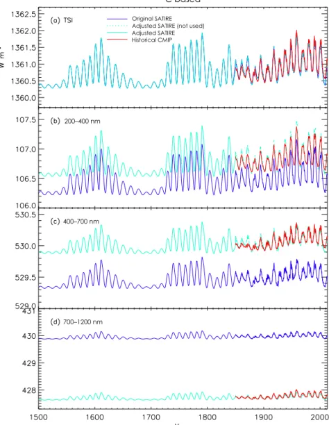
Both irradiance models employ semi-empirical model at- mospheres to describe the brightness spectra of the various solar surface components (sunspots, faculae, networks) responsible for solar irradiance variability on timescales of days to millennia. This allows the consistent reconstruction of both TSI and SSI without relying on SSI measurements. The reconstructions agree with measurements in periods where the latter are considered reliable (cf. Ermolli et al., 2013; Yeo et al., 2015). All provided reconstructions are nor- malised to give the revised absolute TSI level of 1361 W m⁻² during the most recent activity minimum in 2008, as mea- sured by SORCE/TIM (Kopp, 2014). Differences in the secular variations in TSI (Fig. 3) are mainly due to the assumptions made in the irradiance models. The new PMOD-

Figure 3.Reconstructions of total solar irradiance based on two different isotope data sets and two different irradiance models. The 14C-based reconstruction of sunspot numbers is converted to TSI using (black line) the SATIRE-M model and (blue line) the updated Shapiro et al. (2011) model. The¹⁰Be-based TSI reconstruction is constructed using the SATIRE-M model (red line).

based reconstruction features a LMM-to-present amplitude of 3.4 W m⁻² (about 0.25 %), whereas the SATIRE-based forcing changes by less than 1 W m⁻² (0.06 %) during this period. Differences between the¹⁴C- and¹⁰Be-based reconstructions manifest themselves mainly in the phasing and differences in secular trends, for example in the duration and timing of the LMM. The SATIRE-based solar activity reconstruction is also in good overall agreement with a solar activity reconstruction that is exclusively based on cosmic ray measurement/proxy data via a combination of¹⁴C and neu- tron monitor data (Muscheler et al., 2016).

To achieve a smooth transition from the pre-industrial to modern periods, the reconstructions are combined (see Ap- pendix A4.2 for details) with the solar forcing records recommended for the CMIP6historicalexperiment (Matthes et al., 2017). This transition is essentially straightforward for TSI. However, some artefacts cannot be avoided for SSI. The CMIP6historical solar forcing is derived from an average of two conceptually different models, NRLSSI-2 (Codding- ton et al., 2015) and SATIRE, where the latter is a splice of SATIRE-T, based on sunspot observations before 1874 CE (Krivova et al., 2010), and SATIRE-S, based on solar full- disc magnetograms afterwards (Yeo et al., 2014). Differences between the NRLSSI and SATIRE models are discussed by Yeo et al. (2015). Averaging the two intrinsically different SSI series yields a record in which the shape of the solar spectrum does not conform to either model or to observations, e.g. the ATLAS3 (Thuillier et al., 2003) or WHI (Woods et al., 2009) quiet Sun reference spectra.

The SSI records provided for the PMIP4 experiments are a combination of the rescaled reconstructions before 1850 CE, shown for the¹⁴C-based SATIRE reconstruction data set as the cyan solid line in Fig. 4, and the CMIP6 time series for thehistorical simulations (Matthes et al., 2017), shown by the red line. Details of the rescaling and adjustment can be found in Appendix 4.2. Compared to the original reconstruction, the CMIP6 record underestimates the variability in

(13)

200–400 nm

400–700 nm

700–1200 nm

Original SATIRE Adjusted SATIRE (not used) Adjusted SATIRE Historical CMIP

14C based

Figure 4.Adjustment of the¹⁴C/SATIRE-based reconstruction to the CMIP6 historical forcing (Matthes et al., 2017). TSI(a)and SSI(b–

d)in three broad spectral intervals (in the UV between 200 and 400 nm, in the visible at 400–700 nm, and in the near-IR at 700–1200 nm wavelength). The blue lines are the original¹⁴C/SATIRE-based time series, the cyan lines represent the adjusted data, and the red line is the CMIP6 forcing.

the UV after 1850 CE by about 10–15 %, and by more than 35 % if compared to PMOD (not shown), while it overesti- mates the variability in the visible and IR by about 10–15 % and by more than 40 %, respectively. While adjusting the pre-industrial reconstruction to the CMIP6 historical records yields a smooth transition in 1850 CE, it needs to be kept in mind that the amplitude of the variability in the spectral bands is adopted from the original models (i.e. from isotope- based reconstructions before 1850 CE and the CMIP6 record afterwards) and depends at least partly on the construction of the data set. In addition to the standard (adjusted to CMIP6)

14C data sets, we therefore also provide the original records for the entire period for testing the climatic effects of the con- flation.

In summary, PMIP4 provides three reconstructions of TSI and SSI from the most-up-to-date records of cosmogenic ra- dioisotopes ¹⁴C and ¹⁰Be using a chain of models, all of which have been improved and updated since PMIP3. In contrast to CMIP3, for all provided reconstructions, total and spectral irradiance are computed in a self-consistent man- ner. In particular, the same model has been used to reconstruct irradiance from each radioisotope to allow an estimate of the uncertainty due to the effect of local conditions on their formation and deposition. Two irradiance reconstructions were obtained from¹⁴C data using different irradiance models to allow for sensitivity experiments testing the response to the amplitude of the solar forcing. The default forcing for CMIP6-PMIP4past1000 is the¹⁴C SATIRE-based

(14)

reconstruction. The PMOD-based reconstruction provides an upper limit on the magnitude of the long-term changes in irradiance. Since the historical CMIP6 recommendation is an arithmetic average of two conceptually different models with significant differences in the SSI variability, special care has been taken to combine the PMIP4 data sets with the historical forcing. The approach we have chosen here allows for a smooth transition but might nevertheless produce some artefacts.

Apart from the direct effect of changes in TSI and SSI, solar variability also affects stratospheric and mesospheric ozone abundances (e.g. Haigh, 1994) and can contribute significantly to the total stratospheric heating response. In climate models including interactive chemistry, the photolysis scheme should adequately simulate the ozone response to variations in the UV part of SSI. CMIP6 models that do not include interactive chemistry should prescribe ozone variations consistent with the solar forcing and apply a scaling approach similar to the one recommended for the historical period (Matthes et al., 2017; Maycock et al., 2017). It should be noted that solar-ozone regression coefficients as provided by Maycock et al. (2017) have been calculated with respect to the 10.7 cm radio flux (F10.7), which is not available for the PMIP period. Hence we have re-performed the regression of the same ozone fields but with respect to solar UV irradiance averaged over the spectral range from 200 to 320 nm (see Appendix 4.3 for details). We recommend calculating time-varying ozone input for PMIP4 by scaling these coefficients with the anomaly of the respective UV flux during the simulation period and adding it to the CMIP6 pre-industrial ozone climatology. The UV flux anomaly should accordingly be calculated with respect to the CMIP6 pre-industrial irradiance data (Matthes et al., 2017).

4.5 Land use changes and anthropogenic land cover changes

For the past1000 simulation, land use changes need to be implemented using the same input data sets and methodology as the historical simulations; the CMIP6 land use forcing data sets now cover the entire period 850–2015 CE (Hurtt et al., 2017), which provides a seamless transition between the CMIP6 past1000andhistorical simulations. The new land use forcing, Land-Use Harmonization 2 (LUH2), is provided as a contribution of the Land-Use Model Intercomparison Project (LUMIP) to CMIP6 (https://cmip.ucar.edu/lumip).

The LUH2 strategy estimates the fractional land use patterns, underlying land use transitions, and key agricultural man- agement information, annually for the period 850–2100 CE at 0.25^◦×0.25^◦ spatial resolution. The estimate minimises the differences at the transition between the historical reconstruction and the conditions derived from integrated assessment models (IAMs). It is based on new estimates of gridded cropland, grazing lands, urban land, and irrigated land, from the Historical Land Use Data Set for the Holocene

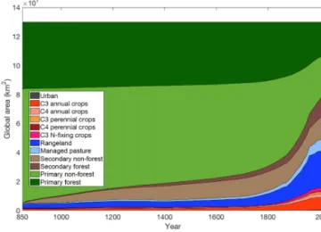
Figure 5.Evolution of various types of land cover and land use changes over the pre-industrial millennium.

(HYDE3.2, Klein Goldewijk, 2016). Within HYDE3.2, grazing lands are now sub-divided into managed pasture and rangeland categories, and irrigated land also includes a sub- category of land flooded for paddy rice. Within LUH2, cropland area is sub-divided into five crop functional types based on data from Monfreda et al. (2008) and from the Food and Agricultural Organization of the United Nations (FAO). The temporal evolution of the various types is displayed in Fig. 5.

LUH2 includes a new representation of shifting cultivation rates and patterns and also includes new layers of manage- ment information such as irrigated area and industrial fer- tiliser usage.

As wood was the primary fuel and an important construction material for nearly all societies in the pre-industrial world, LUH2 includes new scenario reconstructions of wood consumption for the period 850 to 2014 CE. To build these scenarios, an estimate of a baseline wood demand following McGrath et al. (2015) was compiled. To account for differences between continents and technology-induced changes in consumption patterns over time, the wood demand was scaled by historical, country-level estimates of gross domes- tic product (GDP) (Maddison, 2003; Bolt and van Zanden, 2014) (see Appendix A5.1 for details).

As in PMIP3-CMIP5, the default land use data set is at the lower end of the spread in estimates of early agricultural area indicated by other reconstructions (Pongratz et al., 2008; Kaplan et al., 2011). In turn, the lower estimate of early agricultural area at the beginning of the last millennium im- plies larger land-use-induced land cover changes over time to match the land cover distribution of the industrial era (see Schmidt et al., 2012). To allow an assessment of the substantial uncertainties associated with reconstructing historical land use, while at the same time remaining consistent with the format of the default data set, maximum and minimum alternative reconstructions of the LUH2 data set will also be provided during the course of PMIP4. In particu-