Effects of Detached Seaweeds on Structure and Function of Arctic

(1)

fmars-08-575885 February 19, 2021 Time: 19:1 # 1

ORIGINAL RESEARCH published: 25 February 2021 doi: 10.3389/fmars.2021.575885

Edited by:

Susana Carvalho, King Abdullah University of Science and Technology, Saudi Arabia

Reviewed by:

Francesca Rossi, Centre National de la Recherche Scientifique (CNRS), France Christian Wiencke, Alfred Wegener Institute Helmholtz Centre for Polar and Marine Research (AWI), Germany David M. Paterson, University of St Andrews, United Kingdom

*Correspondence:

María José Díaz maguirre@awi.de

Specialty section:

This article was submitted to Marine Ecosystem Ecology, a section of the journal Frontiers in Marine Science

Received:24 June 2020 Accepted:04 February 2021 Published:25 February 2021 Citation:

Díaz MJ, Buschbaum C, Renaud PE and Molis M (2021) Effects of Detached Seaweeds on Structure and Function of Arctic Intertidal Soft-Bottom Communities.

Front. Mar. Sci. 8:575885.

doi: 10.3389/fmars.2021.575885

Effects of Detached Seaweeds on Structure and Function of Arctic

Intertidal Soft-Bottom Communities

María José Díaz^1,2* , Christian Buschbaum³, Paul E. Renaud^4,5and Markus Molis^1,6

1Section of Functional Ecology, Alfred Wegener Institute, Helmholtz-Zentrum für Polar- und Meeresforschung, Bremerhaven, Germany,²Faculty of Biology and Chemistry, University of Bremen, Bremen, Germany,³Wadden Sea Station Sylt, Alfred Wegener Institute, Helmholtz-Zentrum für Polar- und Meeresforschung, Bremerhaven, Germany,⁴Akvaplan-niva, Fram Centre for Climate and the Environment, Tromsø, Norway,⁵Department of Arctic Biology, University Centre in Svalbard, Longyearbyen, Norway,⁶Department of Arctic and Marine Biology, UiT The Arctic University of Norway, Tromsø, Norway

Expected lower sea-ice cover and increased storm frequency have led to projections of an increase in seaweed detritus in Arctic marine systems in the near future. To assess whether detached seaweed affects structural and functional traits of species assemblages in soft-bottom habitats, comparable experiments were run in two intertidal sites (Longyearbyen and Thiisbukta) on Svalbard. At each site, we fixed nets containing the locally dominating seaweeds Saccharina latissima and Desmarestia aculeata (Thiisbukta) orFucussp. (Longyearbyen) to intertidal mud flats. Empty nets were fixed as procedural controls at both sites. After 2.5 months, one sediment core was taken from each manipulated plot and the number of individuals, dry mass, and average length of each encountered animal taxon were recorded. The same measurements were taken from cores collected from unmanipulated areas at each site, both at the start and end of the experiment. Abundance data were used to calculate estimates of diversity (Shannon-index, evenness, and taxon richness), while initial and final average length measurements were used to estimate taxon-specific growth. Log response ratios of initial and final abundance in unmanipulated areas were used to estimate magnitude and direction of the effect of change in community traits over time, serving as a reference to log response ratios estimating manipulated seaweed effects. In Longyearbyen, the presence of detached seaweeds reduced abundance and dry mass by, on average, 46 and 70%, respectively, compared to unmanipulated benthic communities. In Thiisbukta, the presence of seaweeds enhanced evenness, on average by 16%, but reduced abundance and growth of benthic fauna by, on average, 31 and 86%, respectively.

Seaweed effects were generally smaller in Thiisbukta than in Longyearbyen. At both sites, time effects were generally opposite in direction to those caused by the seaweed treatments, yet of similar or larger magnitude. Through reversing temporal dynamics of several of the tested community traits, detached seaweeds strongly modified the structure and functioning of soft-bottom species assemblages at both intertidal sites.

We suggest that the detected effects possibly result from seaweed-induced changes in environmental conditions and/or physical disturbance as underlying processes.

Keywords: Svalbard, habitat connectivity, disturbance, climate change, biodiversity, benthos, Arctic biota, Biotic drivers

Frontiers in Marine Science | www.frontiersin.org 1 February 2021 | Volume 8 | Article 575885

(2)

INTRODUCTION

Over the past 50 years, Arctic warming has exceeded the global average by a factor of two (Parkinson and Comiso, 2013). In Svalbard, summer and winter temperatures have increased by 0.35 and 1.58^◦C per decade, respectively, since 1971 (Hansen- Bauer et al., 2019), faster than in most other regions on Earth.

Global warming may strongly impact Arctic marine ecosystems by promoting a poleward shift in species distributions (Molinos et al., 2015; Hastings et al., 2020) and altered predator-prey relationships (Arctic Monitoring and Assessment Programme [AMAP], 2017). Despite being the primary recipient of warming- induced changes in fluxes of energy and matter (Eakins and Sharman, 2010), the coastal zone of the Arctic has been considered “systematically understudied” (Fritz et al., 2017).

Hence, to improve predictions on the consequences of climate change on nearshore Arctic ecosystems, it is essential to identify the direct and indirect drivers of coastal ecology and unravel their mode of action.

One direct consequence of a warmer Arctic is the decline in sea-ice thickness, extent, and persistence (Serreze and Meier, 2018; Hansen-Bauer et al., 2019). On the one hand, this causes an increase in cumulative photosynthetic active irradiance underwater (Scherrer et al., 2018), leading to better conditions for photoautotrophs (Clark et al., 2013). Benthic seaweed are considered prime profiteers of sea-ice loss in polar seas (Filbee- Dexter et al., 2019) and this notion is corroborated by empirical evidence on the positive relationships between decreasing sea- ice cover and (i) increasing seaweed abundance in two Svalbard fjords (Kortsch et al., 2012), (ii) an extension of kelp depth range (Krause-Jensen et al., 2012), and (iii) increased biomass production of kelp in Greenland (Krause-Jensen et al., 2012) and Svalbard (Bartsch et al., 2016) in recent years. On the other hand, the loss of protective sea-ice will also intensify the level of wave exposure (e.g.,Vermaire et al., 2013;Filbee-Dexter et al., 2019) and, hence, mechanical stress on the biota of Arctic coastal zones (Krause-Jensen and Duarte, 2014). On rocky shores, this will apply to many species of seaweed, in particular kelp and intertidal algae, which comprise some of the largest sessile organisms present. Kelp detachment rates generally exceed 50%

of their annual biomass production (Krumhansl and Scheibling, 2012) and will potentially increase in the future due to the predicted increase in the frequency and intensity of storms at higher latitudes (Sepp and Jaagus, 2011).

Dislodged seaweeds may disperse long distances before accumulating on-shore or in deeper basins (Harrold et al., 1998).

For instance, Filbee-Dexter et al. (2018) reported that detrital kelp was present in half of the observations made at depths of 65–85 m in a fjord in northern Norway, i.e., below the vertical distribution limit of attached conspecifics (Filbee-Dexter et al., 2019). As such, detached seaweeds serve as vectors connecting rocky shores with intertidal as well as subtidal habitats, including sedimentary shores, where they can affect the ecology of recipient communities in a number of ways (Krumhansl and Scheibling, 2012). First and most intensely studied, detached seaweeds may be an detrital food source for recipient benthic communities (Filbee-Dexter and Scheibling, 2012; Renaud et al., 2015), which

may modify food web structure of the subsidized communities (e.g.,Piovia-Scott et al., 2011). In Antarctica, for instance,Norkko et al. (2004)demonstrated thatPhyllophoradrift accumulation has a structuring role on soft-sediment communities through organic food subsidies. Second, detached seaweeds increase structural complexity, particularly in shallow sedimentary areas, thereby providing refuge for epibenthic organisms from predators such as fish in subtidal habitats (Langtry and Jacoby, 1996; Norkko and Bonsdorff, 1996b) or wading birds in the intertidal (Lewis et al., 2003). Third, movements of detached seaweeds may physically disturb sediment-dwelling animals, leading to a decrease in the number of taxa and individuals (Petrowski et al., 2016). Finally,Norkko and Bonsdorff (1996a) andCardoso et al. (2004)reported that oxygen deficiencies in the sediment arose upon extended periods of seaweed coverage in the Baltic Sea and Atlantic coast of Portugal, respectively.

In sharp contrast to the temperate zone, the ecology of intertidal communities in the Arctic has been understudied.

The few exceptions to this are nearly exclusively observational studies with little evidence about the underlying processes (reviewed inMolis et al., 2019). Climate-driven projections of change in Arctic marine systems suggest that stranded seaweeds will be of greater relevance in the future, through e.g., the contribution of organic matter, access to shelter for mobile predators, mechanical disturbance or impeding water and oxygen flow. However, their effects on the function and structure of polar intertidal communities are unknown. Here, we use manipulative experiments conducted in two Svalbard fjords to test the hypothesis that the presence of detached seaweeds will affect structure and functioning of intertidal benthic assemblages.

In addition, we strive for some level of generality in quantifying magnitude and direction of the effects of the presence of detached seaweeds on structural (diversity, total abundance, species composition) and functional traits (growth, biomass) of soft-bottom animal communities. Changes in manipulated plots are compared in magnitude and direction with the changes in time (i.e., between start and end of the experiment).

MATERIALS AND METHODS Study Sites

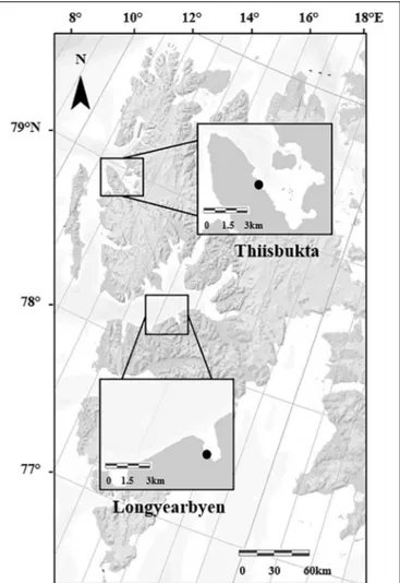
This study was conducted on two intertidal sedimentary shores in Svalbard, Norway (Figure 1). The first site, “Longyearbyen”

(N 78.22351^◦, E 15.67043^◦) is located in Adventfjorden, which is one of the southern arms of Isfjorden. Two rivers, Adventelva and Longyearelva, discharge into the innermost part of Adventfjorden. The intertidal area studied is an extended plain of sand and mud (Elverhøi et al., 1983) with an average tidal amplitude of 2.1 m. Measurements at the University Centre in Svalbard (UNIS) CTD station in Adventalen reveal annual fluctuations in sea surface temperature between 1.1 and 8^◦C and in salinity between 31.7 and 35.3 units. Located approximately 100 km north of Longyearbyen, the second site,

“Thiisbukta” (N 78.92798^◦, E 11.90344^◦), is on the southern shore of Kongsfjorden. The substrate here is fine sand mixed with coarse silt (mean ± SD grain size: 67.8 ± 25.0 µm)

(3)

Díaz et al. Effects of Detached Seaweeds on Arctic Communities

(Ambrose and Leinaas, 1988;Bick and Arlt, 2005). Temperature and salinity at 0–5 m water depth ranged from 2.9 to 7.7^◦C and 31.8–35.1, respectively (Fischer et al., 2018). Both parameters are affected by glacial discharge into Kongsfjorden (Svendsen et al., 2002). The average tidal amplitude in Kongsfjorden is 1.8 m (Svendsen et al., 2002).

Experimental Design and Set-Up

To evaluate the effects of detached seaweeds on structure and functioning of intertidal soft-bottom communities, a factorial experiment with complete randomized blocks was set up in Thiisbukta on 23 May and in Longyearbyen on 1 June 2017.

Each experiment was installed during one low tide at ca. 1 m above mean low tide level, leaving plots emerged during each low tide for approx. 4 h. At each site, six blocks were established at a minimum distance of 7 m to the nearest block. Each block (3.5 × 3.5 m) contained three treatments in duplicate (= six experimental units [EUs] per block), resulting in 36 EUs in total per site. In each block, treatments were randomly allocated to

FIGURE 1 |Map of the Svalbard Archipelago with marked study areas, and the black points indicate the study sites Longyearbyen and Thiisbukta (Norwegian Polar Institute/https://geokart.npolar.no/).

EUs (50×50 cm) which were separated by a minimum distance of 1 m (Figure 2). The first treatment simulated the presence of detached seaweeds (= seaweed mat). In Longyearbyen, the intertidal algaFucussp. was the only seaweed encountered, while in Thiisbukta, stranded seaweeds were composed of a mix of S. latissima(70%) andD. aculeata(30%). Twelve seaweed mats were produced by filling 12 black polyethylene nets (50×50 cm, with 8 cm mesh size) on average with 1300 ± 50 g (± SD) of naturally available detached seaweeds (as described in the previous sentence) that were collected during low tide from the intertidal of each site. The second treatment conferred the assessment of artifacts (= procedural control), by deploying two empty nets per block. To permanently fix nets to the ground, six iron bars (35 cm length with a 5 cm long top end bend) were pushed completely into the sediment along the net margin, including each corner of a net. The third treatment consisted of unmanipulated areas. The experiments in Thiisbukta and Longyearbyen ran until 8 and 23 August 2017, respectively.

Collection and Processing of Samples

Two sediment cores were taken from each unmanipulated area of each block at the start and at the end of the experiment (n = 2 samples per block × 6 blocks = 12 at each site and each time point). Moreover, one sample was taken from the center of each procedural control (n= 2×6) and below each seaweed mat (n = 2 × 6) at the end of the experiment. All samples were collected by pushing a sediment corer of 5.4 cm diameter 10 cm deep into the sediment (method adopted from Petrowski et al., 2016). Samples were transported within 1 h of collection to UNIS (Longyearbyen) or the Marine Laboratory in Ny-Ålesund (Thiisbukta) and stored at 4^◦C until processing (maximum of 48 h after sampling). Processing started by gently

FIGURE 2 |Schematic spatial arrangement (not to scale) of a block hosting duplicate experimental units (quadrates) of each “Detached seaweed”

treatment (dark gray), procedural control (light gray), and unmanipulated areas (white). Arrows with numbers indicate distances. Dashed line indicates intended block margin.

(4)

rinsing each core with a slow-flowing jet of seawater over a sieve with 0.5 mm mesh size to isolate organisms from the sediment. All intact, living animals were identified to the lowest possible taxonomic level, usually to species level, using a stereomicroscope. Headless polychaete fragments were omitted from abundance data to minimize the risk of overestimating polychaete abundances, but included for biomass quantification.

To estimate structural community responses, abundance, taxon richness, Shannon index (to natural logarithm), and Pielou’s evenness of each sample were calculated.

To quantify growth, maximum length of 10 undamaged individuals of each taxon of each sample was measured to the nearest 1 mm at the beginning (then only unmanipulated areas could be sampled) and end of the experiment (from unmanipulated areas and plots covered with an empty net or a seaweed mat). For taxa with <10 individuals per sample, the lengths of all individuals were recorded and the average length of each taxon per sample calculated. Taxon-specific estimates of change in length were calculated as (L_f – Li)/Li, where L_f and Li are the average length of organisms collected at the end and start of the experiment, respectively. For each sample, all taxon- specific estimates of change in length were summed to yield a replicate measurement of length change (hereafter growth) for statistical analyses. After drying all organisms of a sample at 60^◦C to constant weight, dry mass was quantified to the nearest 0.001 g with a laboratory balance (Mettler-Toledo). At the end of the experiment, average (±SD) seaweed residual biomass of each EU hosting a seaweed mat treatment was 116 g (± 44) in Longyearbyen and 105 g (± 55) in Thiisbukta. In each of two plots of the detached seaweed treatment in Thiisbukta, one specimen (4.3 and 5.1 cm total length) of Arctic staghorn sculpin (Gymnocanthus tricuspis) was found among algal remains.

Data Analysis

Following editorial recommendations in a special issue of “The American Statistician” on statistical inference (Vol. 73, No. S1), we avoid using the term “statistically significant” and any of its variants (Wasserstein et al., 2019). Furthermore, we opted not to usep-values in making dichotomous decisions at the level of α≤0.05 rather we consideredp-values as a continuous metric of probability that the calculated value of a test statistic occurred by chance alone, given that the null hypothesis is correct (Crawley, 2013, p. 753). Where homoscedasticity of residuals was likely, data were square root transformed to meet the assumptions.

We calculated with mixed model ANOVAs whether (i) treatment effects of (i) seaweeds (two levels, fixed: seaweed- cover plots vs. unmanipulated areas) or (ii) an artifact (2 levels, fixed: empty net-covered plots vs. unmanipulated areas) on taxon richness, Pielou’s evenness, Shannon index, abundance, dry mass, and growth were independent of the location of blocks (six levels, random) at the study site (see “S × B”

interaction inAppendix Table A1), using the R package “GAD”

(Sandrini-Neto and Camargo, 2012). Subsequently, we assessed three types of effects for each of the six above listed response variables. Firstly the effect of detached seaweeds was evaluated by comparing data collected in seaweed-covered plots and unmanipulated areas (hereafter seaweed effect). Secondly the

artifact effect was assessed by comparing data collected in net-covered plots and unmanipulated areas (hereafter artifact).

Differences in the values of a response between both treatments indicate that the net itself may have an effect on that community response. Thirdly the underlying time effect was quantified for each response variable, except growth for which this was not possible, by comparing data collected in unmanipulated areas at the end and start of the experiment (hereafter time effect). The time effect constitutes a measure of natural change and serves as a reference for seaweed effects, which resulted from the manipulation. For each community response, we calculated five statistical metrics to evaluate the likelihood of an effect. (i) With a Student’s t-test we estimated the value of the test statistic t and its probability (p), using the function “t-test” of the R package “stats” v3.5.1 (Pinheiro et al., 2018). (ii) Test power of t-tests was quantified, using the “pwr.t.test” function of the R package “pwr.2” v1.0 (Lu et al., 2017). (iii) The minimum false positive risk (mFPR), for which the prior probability of there being a real effect was set according to the recommendation by Colquhoun (2019) to 0.5. The mFPR estimates the probability (scale 0–

1) of obtaining an observed test statistic by chance alone.

It was calculated with the “calc.FPR” function, provided in the script “Cushny-t-test+FPR.R” (SupplementalColquhoun, 2019). (iv) The Bayes factor (BFA0), a ratio indicating the likelihood of data fit under the alternative relative to the null hypothesis, using the “ttest.tstat” function of the R package “BayesFactor” v0.9.12–4.2 (Morey et al., 2018). (v) The average log response ratio (LRR) as the decadal logarithm of the quotient of means of the above primary and secondary treatments (see above description on seaweed effect, artifact, and time effect) as nominator and denominator, respectively, using the “escalc” function of the R package “metafor” v2.0- 0 (Viechtbauer, 2010). Average LRRs were plotted with their 95% confidence interval (CI) using the “forest” function in “metafor.”

Normality of residuals was formally checked with the Shapiro-Wilks test and graphically by quantile-quantile plots. Homogeneity of variances was formally checked with Cochran’s test using the “C-test” function of the R package

“GAD” v1.1.1 and graphically through missing trends in the residuals with fitted values (Crawley, 2013, p. 405).

Heteroscedasticity inflates the type II error rate and, thus needs to be considered only where treatment effects occur (Underwood, 1997). This was the case in four tests (marked by a T in Tables 2, 3). For each site, we separately tested for seaweed effects as well as artifacts and time effects on taxon composition by calculating the respective Bray-Curtis similarity indices on untransformed relative abundances.

Using relative abundances of taxa rather than the absolute value of abundances provides an unbiased measurement on compositional differences by excluding differences in overall counts (Greenacre, 2018). We run three separate mixed model PERMANOVAs (9999 permutations) to calculate the probability of main and interactive effects of block (6 levels, random) with either (i) seaweed treatments (2 levels, fixed:

seaweed-covered vs. unmanipulated plots), or (ii) artifact

(5)

fmars-08-575885February19,2021Time:19:1#5

Díazetal.EffectsofDetachedSeaweedsonArcticCommunities

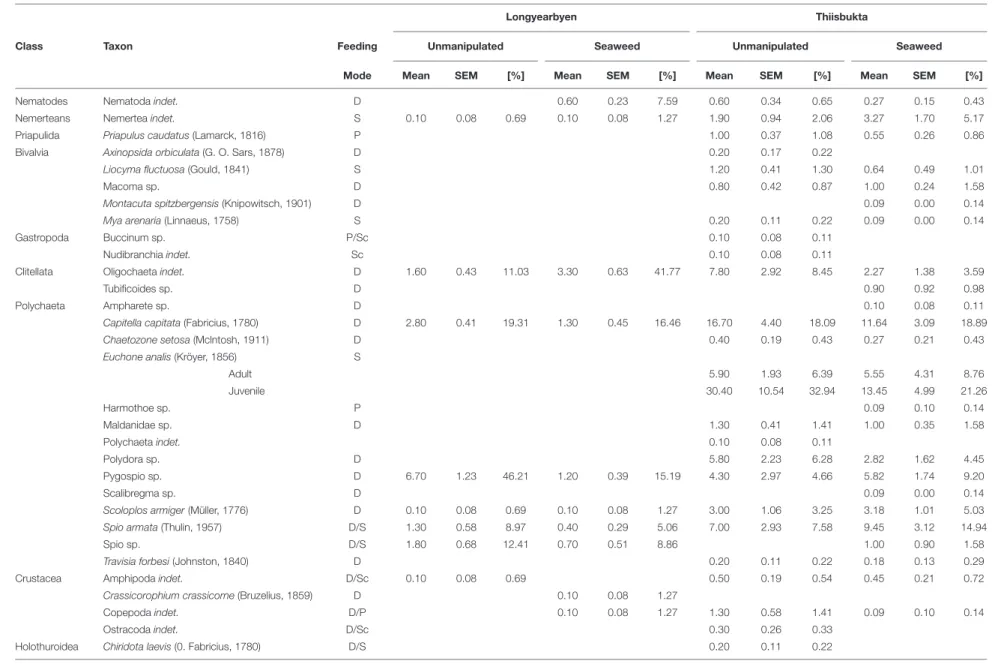
TABLE 1 |Mean and standard error of the mean (SEM) number of individuals of each taxon encountered in samples taken from plots covered with detached seaweeds and unmanipulated areas at the end of 83–81 days experiments in Longyearbyen and Thiisbukta, respectively.

Longyearbyen Thiisbukta

Class Taxon Feeding Unmanipulated Seaweed Unmanipulated Seaweed

Mode Mean SEM [%] Mean SEM [%] Mean SEM [%] Mean SEM [%]

Nematodes Nematodaindet. D 0.60 0.23 7.59 0.60 0.34 0.65 0.27 0.15 0.43

Nemerteans Nemerteaindet. S 0.10 0.08 0.69 0.10 0.08 1.27 1.90 0.94 2.06 3.27 1.70 5.17

Priapulida Priapulus caudatus(Lamarck, 1816) P 1.00 0.37 1.08 0.55 0.26 0.86

Bivalvia Axinopsida orbiculata(G. O. Sars, 1878) D 0.20 0.17 0.22

Liocyma fluctuosa(Gould, 1841) S 1.20 0.41 1.30 0.64 0.49 1.01

Macoma sp. D 0.80 0.42 0.87 1.00 0.24 1.58

Montacuta spitzbergensis(Knipowitsch, 1901) D 0.09 0.00 0.14

Mya arenaria(Linnaeus, 1758) S 0.20 0.11 0.22 0.09 0.00 0.14

Gastropoda Buccinum sp. P/Sc 0.10 0.08 0.11

Nudibranchiaindet. Sc 0.10 0.08 0.11

Clitellata Oligochaetaindet. D 1.60 0.43 11.03 3.30 0.63 41.77 7.80 2.92 8.45 2.27 1.38 3.59

Tubificoides sp. D 0.90 0.92 0.98

Polychaeta Ampharete sp. D 0.10 0.08 0.11

Capitella capitata(Fabricius, 1780) D 2.80 0.41 19.31 1.30 0.45 16.46 16.70 4.40 18.09 11.64 3.09 18.89

Chaetozone setosa(Mclntosh, 1911) D 0.40 0.19 0.43 0.27 0.21 0.43

Euchone analis(Kröyer, 1856) S

Adult 5.90 1.93 6.39 5.55 4.31 8.76

Juvenile 30.40 10.54 32.94 13.45 4.99 21.26

Harmothoe sp. P 0.09 0.10 0.14

Maldanidae sp. D 1.30 0.41 1.41 1.00 0.35 1.58

Polychaetaindet. 0.10 0.08 0.11

Polydora sp. D 5.80 2.23 6.28 2.82 1.62 4.45

Pygospio sp. D 6.70 1.23 46.21 1.20 0.39 15.19 4.30 2.97 4.66 5.82 1.74 9.20

Scalibregma sp. D 0.09 0.00 0.14

Scoloplos armiger(Müller, 1776) D 0.10 0.08 0.69 0.10 0.08 1.27 3.00 1.06 3.25 3.18 1.01 5.03

Spio armata(Thulin, 1957) D/S 1.30 0.58 8.97 0.40 0.29 5.06 7.00 2.93 7.58 9.45 3.12 14.94

Spio sp. D/S 1.80 0.68 12.41 0.70 0.51 8.86 1.00 0.90 1.58

Travisia forbesi(Johnston, 1840) D 0.20 0.11 0.22 0.18 0.13 0.29

Crustacea Amphipodaindet. D/Sc 0.10 0.08 0.69 0.50 0.19 0.54 0.45 0.21 0.72

Crassicorophium crassicorne(Bruzelius, 1859) D 0.10 0.08 1.27

Copepodaindet. D/P 0.10 0.08 1.27 1.30 0.58 1.41 0.09 0.10 0.14

Ostracodaindet. D/Sc 0.30 0.26 0.33

Holothuroidea Chiridota laevis(0. Fabricius, 1780) D/S 0.20 0.11 0.22

Empty cells indicate absence of organisms. Feeding mode classification: D, deposit feeder; S, suspension feeder; P, predator; Sc, scavenger.

“%” = proportion of individuals of a taxon to the total number of individuals encountered in all samples of this treatment, n = 12, “Unmanipulated” = absence of detached seaweeds, “Seaweed” = presence of detached seaweeds.

FrontiersinMarineScience|www.frontiersin.org5February2021|Volume8|Article575885

(6)

TABLE 2 |Longyearbyen.

Response Effect t P power mFPR BFA0 Shap Coch

Richness Seaweed 1.60 0.123 0.36 0.366 0.79 0.042 0.051

Artifact –0.19 0.855 0.05 0.663 0.29 0.025 0.169

Time 7.35 <0.001 1.00 0.000 >500 0.013 0.454

Evenness Seaweed 0.78 0.442 0.12 0.595 0.37 <0.001 0.002

Artifact –0.36 0.723 0.06 0.652 0.30 0.352 0.169

Time 2.27 0.035 0.61 0.162 1.78 0.031 0.005

Shannon Seaweed 1.42 0.171 0.29 0.428 0.65 0.088 0.014

Artifact –0.11 0.917 0.05 0.665 0.29 0.192 0.332

Time 7.99 <0.001 1.00 0.000 >1,000 0.457 0.738

Biomass Seaweed (T) 3.30 0.003 0.91 0.022 7.84 0.410 0.621

Artifact 0.27 0.791 0.06 0.658 0.30 0.003 0.591

Time (T) 3.15 0.005 0.88 0.031 5.48 0.051 0.036

Abundance Seaweed 2.72 0.013 0.78 0.072 3.38 0.313 0.440

Artifact 0.24 0.814 0.06 0.660 0.30 0.355 0.881

Time 2.70 0.014 0.77 0.077 3.08 0.150 0.274

Growth Seaweed na na na Na na na na

Artifact 3.88 <0.001 0.97 0.006 18.05 0.985 0.273

Summary of statistical analyses of univariate responses. t = test statistic of Student’s t-test, p = probability of test statistic t, power = probability of making a type II error (Student’s t-test), mFPR = minimum false positive risk as the probability that the result is due to chance, BFA0= Bayes factor as evidence for the alternative hypothesis, Shap = p-value of Shapiro-Wilks test for normality, Coch = p-value of Cochran’s-test.

Clear results sensuDushoff et al. (2019)in bold font. (T) = data transformed by square root, na = not analyzed due to artifact and block×treatment interactions, n = 12.

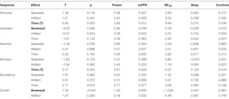
TABLE 3 |Thiisbukta.

Response Effect T p Power mFPR BFA0 Shap Cochran

Richness Seaweed 1.39 0.178 0.28 0.437 0.63 0.263 0.415

Artifact 1.21 0.241 0.22 0.493 0.52 0.208 0.392

Time (T) 3.60 0.002 0.95 0.012 9.69 0.015 0.036

Evenness Seaweed –3.03 0.006 0.86 0.038 5.30 0.328 0.570

Artifact –0.47 0.645 0.08 0.642 0.31 0.752 0.209

Time –1.61 0.122 0.36 0.364 0.83 0.634 0.007

Shannon Seaweed –1.30 0.206 0.86 0.464 5.29 0.836 0.883

Artifact 0.41 0.686 0.07 0.647 0.31 0.651 0.032

Time 0.30 0.765 0.36 0.656 0.83 0.571 0.215

Biomass Seaweed –1.60 0.123 0.31 0.366 0.80 <0.001 0.031

Artifact –1.94 0.065 0.49 0.253 1.18 0.004 0.022

Time (T) 3.17 0.005 0.91 0.034 5.57 0.125 0.070

Abundance Seaweed 1.97 0.062 0.50 0.245 1.22 0.008 0.007

Artifact 0.91 0.372 0.15 0.569 0.41 0.132 0.889

Time 2.71 0.014 0.77 0.077 3.08 0.064 0.126

Growth Seaweed 7.33 <0.001 1.00 0.000 >1,000 0.244 0.381

Artifact 1.07 0.295 0.19 0.530 0.46 0.361 0.149

Summary of statistical analyses of univariate responses. t = test statistic of Student’s t-test, p = probability of test statistic t, power = probability of making a type II error (Student’s t-test), mFPR = minimum false positive risk as the probability that the result is due to chance, BFA0= Bayes factor as evidence for the alternative hypothesis, Shap = p-value of Shapiro-Wilks test for normality, Coch = p-value of Cochran’s-test. Clear results sensuDushoff et al. (2019)in bold font. (T) = data transformed by square root, n = 12.

treatments (2 levels, fixed: empty net vs. unmanipulated plots), or (iii) time treatments (2 levels, fixed: unmanipulated plots at the start and end of the experiment), using the “adonis”

function of the R package “vegan” v2.5–6 (Oksanen et al., 2018). When the probability of a treatment×block interaction was>0.25, the analysis was repeated after pooling the variance of the interaction term with the residual variance of the full

model (Quinn and Keough, 2002). We generated biplots with the “plot” function of R “base” package to illustrate (i) treatment effects along both principle components explaining most of the variation of the data and (ii) loading values for up to 10 of the most influential taxa. All calculations and plotting were done with RStudio Version 1.0.136 (RStudio Team, 2016).

(7)

RESULTS

We identified a total of 31 taxa (11 at Longyearbyen and 30 at Thiisbukta). At both sites, the soft-bottom fauna was dominated by polychaetes. In total, 7 (64%) and 18 (52%) polychaete taxa were encountered in Longyearbyen and Thiisbukta, respectively.

In Longyearbyen,Pygospiospec.,Capitella capitata, oligochaetes, andSpiosp. were the most abundant taxa across all treatments (Table 1). Average abundance of oligochaetes was twofold higher in seaweed-covered plots than in unmanipulated areas. In contrast, the abundance ofPygospiosp.,Spiosp., andC.capitata was in seaweed-covered plots 18, 39, and 46%, respectively, of their abundance in unmanipulated areas. In Thiisbukta, C.

capitata,Spio armata,Pygospiosp., and oligochaetes, i.e. almost the same taxa as in Longyearbyen, contributed strongest to infauna abundance (Table 1). The abundance of oligochaetes and C. capitata in seaweed-covered plots was, on average, 29 and 69%, respectively, of their abundance in unmanipulated areas. Contrarily, the abundance of each,S.armata, andPygospio sp. increased 1.35-fold in seaweed-covered plots compared to unmanipulated areas. For the tube-dwelling polychaeteEuchone analis, which was absent in Longyearbyen, we were able to discriminate between juveniles and adults. When we considered the abundance of both life stages combined, E.analis was the most abundant taxon in Thiisbukta (Table 1). The abundance of juveniles was more strongly reduced by seaweed cover than that of adults, with average declines of 57 and 6%, respectively, relative to unmanipulated areas.

Univariate Response Variables

Block Effects

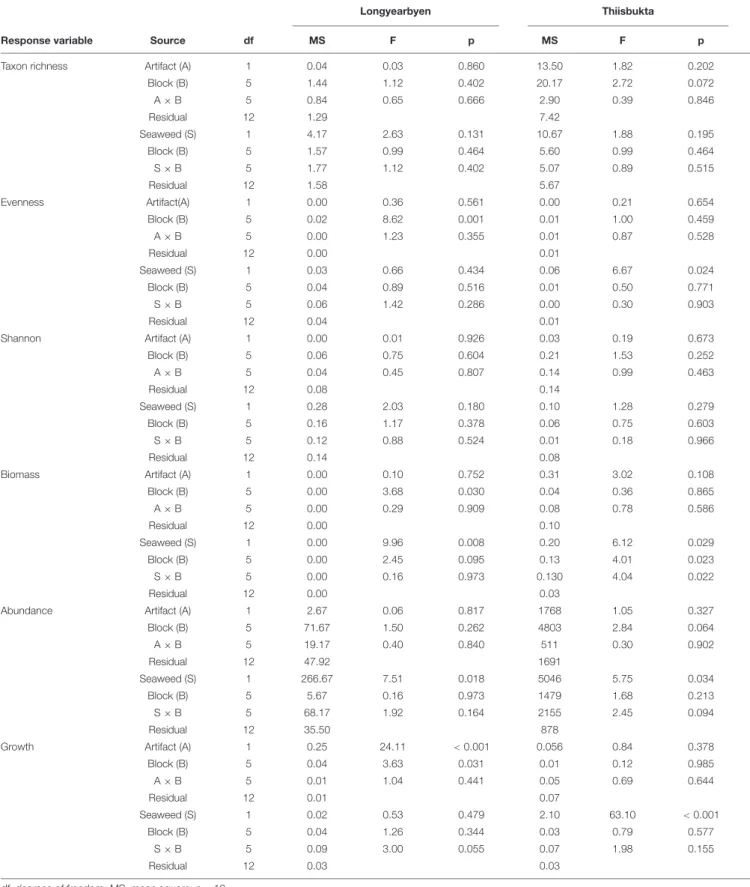
Main block effects are likely for biomass (Longyaerbyen) as well as taxon richness and abundance (both Thiisbukta) (Appendix Table A1), but these results only indicate that these responses varied among some or all blocks. Main block effects do not affect the interpretation of the effects of fixed factors, while the existence of a seaweed×block interaction indicates that seaweed effects on measured responses are dependent on location of plots within the study site. A “treatment×block” interaction seems unlikely for all response variables except biomass in Thiisbukta (Appendix Table A1).

Artifacts

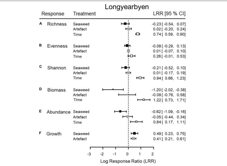
Only for growth in Longyearbyen did statistical analyses support a difference between unmanipulated plots and procedural controls, based on low probability of the t-statistic, underpinned by high test power, low mFPR, and large BFA0 (Table 2). Thus results indicated that these data were about 18 times more likely to occur under the alternative hypothesis of procedural control effects. Furthermore, the LRR of the artifact effect on growth points in the same direction and is of similar magnitude as the LRR of the seaweed effect (Figure 3F), providing strong evidence that the seaweed effect on growth in Longyearbyen was mainly driven by the net itself. As a consequence, we did not perform statistical analyses on Longyearbyen growth data, but plotted the data. For the remaining response variables we found a generally high probability of the t-statistic, although we also found low

test power and a high false positive risk. Furthermore, with the exception of biomass in Thiisbukta, average LRRs were near zero (treatment “Artifact” in Figures 3,5) and BFA0 values in favor of the null hypothesis (Tables 2,3). All this suggests that the net itself had little influence on any detected seaweed effect for all univariate response variables except growth in Longyearbyen.

Diversity Measures

In Longyearbyen, the difference among seaweed treatments is statistically unclear for taxon richness, evenness, and Shannon- index (Table 2), given (i) a test power ≤ 0.36, (ii) a low magnitude of seaweed effects (Figures 3A–C,4A–C), and (iii) a minimum probability of≥37% that results occurred by chance alone (mFRP in Table 2). Furthermore, Bayes factors (BFA0

in Table 2) of 0.8 (taxon richness), 0.4 (evenness), and 0.7 (Shannon-index), indicate that the data were (1/0.8) = 1.25, (1/0.4) = 2.5, and (1/0.7) = 1.4 times, respectively, as likely under the null hypothesis as they are under the alternative hypothesis.

In contrast, the time effect on taxon richness and Shannon-index, but not evenness, showed clear differences between samples taken in unmanipulated areas at the start and end of the experiment (Table 2). A BF_A0>500 for taxon richness and Shannon-index together with maximum test power and lowest possible mFPRs are decisively in favor of the alternative hypothesis (Table 2).

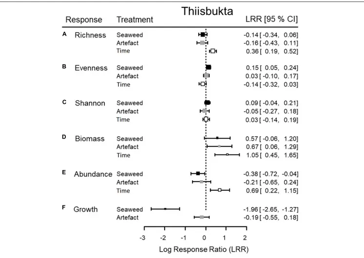
This view is supported by the large, positive time effect of both response variables (Treatment “Time” Figures 3A,C 4A,C). In Thiisbukta, a seaweed effect on taxon richness and Shannon- index was not well supported, due to low test power, a probability of >44% that results occurred by chance (Table 3), and the small effect size (Treatment “Seaweed”Figures 5A,C,6A,C). For evenness, however, a low mFPR, moderate test power, and large Bayes factor support the alternative hypothesis of an, albeit small, seaweed effect (Table 3 andFigures 5B, 6B). Only for taxon richness did a time effect seem plausible (Figures 5,6), given a moderate LRR, high test power, and low false positive risk of the test (Table 3“Richness”).

Biomass, Abundance, and Growth

In Longyearbyen, a strong negative effect of seaweed cover on dry mass (Figures 3D,4D) shows up as the data were 7.8 times more likely to occur under the alternative hypothesis and the minimum probability to obtain the test result by change is 2.2% (Table 2).

Similarly, statistical support exists for a strong time effect on biomass (Table 2) that is of comparable magnitude to the seaweed effect but in the opposite direction (Figures 3, 4D). Regarding total abundance, there is ambiguous statistical evidence for a negative seaweed effect, given the large effect size, a 3.4 times higher likelihood of the alternative hypothesis but also a 7.2%

minimum probability of getting this result by chance (Table 2 and Figures 3E, 4E). The magnitude of the time effect on abundance is comparable to the seaweed effect, but again in the opposite direction (Figures 3E,4E), yet based on equivocal statistical evidence (Table 2). In Thiisbukta, the observed seaweed effect on biomass (Figures 5D, 6D) is statistically unclear due to low test power and a minimum probability of almost 37%

that the result has occurred by chance (Table 3). Furthermore, comparable effect sizes between the seaweed effect and the artifact

(8)

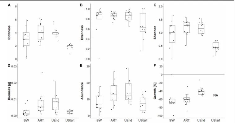
FIGURE 3 |Longyearbyen. Median (thick horizontal line)±SEM (box), 95% confidence interval (vertical line), and sample-wise values (points) of taxon richness(A), evenness(B), Shannon-index(C), biomass(D), abundance(E), and growth(F)of the benthic fauna in core samples (21 cm²surface area) taken in

seaweed-covered (SW), procedural controls (ART), unmanipulated areas at end (UEnd) and unmanipulated area at start (UStart). For growth, “NA” = data not available for areas unmanipulated at start.n=12.

(Figures 5,6D) suggest that the net itself may have caused the observed increase in biomass in seaweed-covered plots. However, there is clear statistical support for a time effect on biomass (Table 3andFigures 5,6D). With respect to abundance, there is no clear seaweed effect, given that the data are 1.2:1 in favor of the alternative hypothesis, a minimum probability of 25% to obtain the test statistic by chance, and low test power (Table 3).

Despite a large effect size (Figures 5,6E) statistical evidence for a positive time effect on abundance is equivocal (Table 3). There is ample statistical support for a strong reduction in growth of animals in seaweed-covered plots relative to fauna sampled in unmanipulated areas (Table 3andFigures 5,6F).

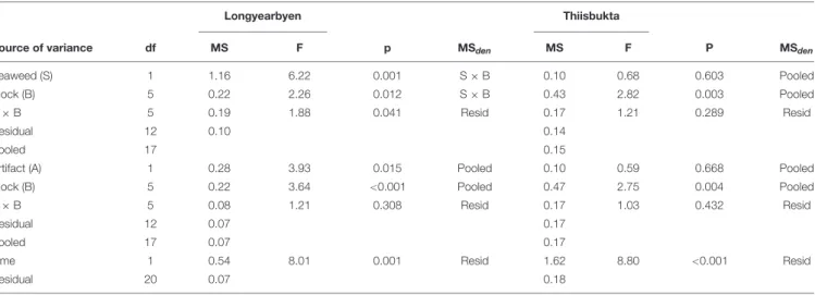
Taxonomic Composition

In Longyearbyen, there is a low probability of the test statistic of the seaweed effect (Table 4). This is, however, also the case for the artifact indicating that the seaweed effect on taxonomic composition may be caused by the net itself. There is also a low probability of the test statistic of the time comparison. Most of the taxa contribute equally strongly to the observed time separation in taxonomic composition of the soft-bottom assemblage in Longyearbyen (Figure 7A). In Thiisbukta, the high probability of the test statistic, given the hypothesis of no differences in species composition between seaweed-covered and unmanipulated plots as well as between net-covered and unmanipulated plots indicates that seaweed cover was unlikely to modify the taxonomic composition of the soft-bottom community. In contrast, a timing

difference in taxonomic composition is very likely (Table 4). The taxa contributing strongest to this change includeMacomasp., Pygospiosp.,P. caudatus, andE. analis(Figure 7B).

DISCUSSION

Time effects were detected for each response variable, often at both sites. This indicates that the duration of the experiment was sufficiently long to allow the development of detectable change in studied community traits. Hence, it seems unlikely that absence of a seaweed effect at the end of the experiment results from the test duration being too short.

Functional Community Responses

Both in Longyearbyen and Thiisbukta, dry mass of infauna increased in unmanipulated areas over the course of the experiment, indicating that living conditions were generally favorable for faunal settlement, growth, and/or immigration at both study sites during the experiment. Besides temporal changes in Longyearbyen, higher mean final dry mass of infauna in unmanipulated areas than in seaweed-covered plots suggests that the presence of seaweeds interfered with infauna biomass accrual. Reduction in biomass accrual in seaweed-covered plots in Longyearbyen was of the same magnitude as the temporal increase in biomass accrual in unmanipulated plots. The lack of a net increase in biomass in seaweed-covered plots might be due to a direct interference of seaweed cover with the

(9)

FIGURE 4 |Longyearbyen. Mean (square) and 95% confidence interval (CI, horizontal whiskers) of logarithmic response ratios (LRR) to quantify the effect of (i) seaweed presence (“Seaweed”; seaweed-covered vs. unmanipulated, black), (ii) procedural controls (“Artifact”; empty net-covered vs. unmanipulated, gray), and (iii) changes in unmanipulated areas over the course of the experiment (“Time”; unmanipulated end vs. unmanipulated start, white), for six(A–F)responses. Dashed line = level of no effect,n=12.

availability of food or the capacity of organisms to capture food.

Moreover, the presence of detached seaweeds may indirectly affect infauna biomass accrual through hampered settlement of fauna or enhanced consumption of fauna due to an accumulation for predators seeking shelter under detached seaweeds (pers.

obs. M Molis). However, an increase in the abundance of some taxa (e.g., oligochaetes) in seaweed-covered plots compared to unmanipulated areas suggests that an accumulation of biomass occurred also in seaweed-covered plots, but was compensated by the loss of several taxa, such asPygospiosp. andC.capitata.

The observed seaweed-mediated decline in net biomass could principally result from numerical responses (e.g., immigration and mortality of individuals), altered performance such as growth rate, or both. Our data suggest two reasons why the presence of seaweeds mainly affected numerical responses. First, magnitude and direction of the seaweed effect on growth (as a proxy of performance) closely match the artifact effect, suggesting the presence of a net rather than seaweeds as a driver of growth.

Second, the seaweed-induced reduction in abundance (as a

surrogate of numerical responses) at the end of the experiment (Figure 2E, “Seaweed”) was comparable in magnitude to the temporal increase in abundance (Figure 2E, “Time”), paralleling the above described developments on biomass.

Several plausible explanations exist regarding this strong numerical response of infauna in seaweed-covered plots. First, seaweed thalli may mechanically interfere with soft-bottom organisms in at least two ways. On the one hand, thalli may obstruct the flow of water transporting food from the water column to the substrate (barrier effect), potentially affecting the supply of food for suspension feeders or recruitment of pelagic larvae. The number of juvenileE. analisin seaweed-covered plots, for instance, was half of that in unmanipulated areas. On the other hand, thallus movements may force infauna to seek refuge in less disturbed areas. Although we fixed all nets with their bottom-facing part to the substrate, scouring of the substrate by wave-induced mat movements were possible.Petrowski et al.

(2016) showed for a subtidal soft-bottom community near Thiisbukta that even sporadic movements of a single kelp thallus

(10)

FIGURE 5 |Thiisbukta. Mean (square) and 95% confidence interval (horizontal whiskers) of logarithmic effect ratios (LRR) to quantify the effect of (i) seaweed presence (“Seaweed”; seaweed-covered vs. unmanipulated, black), (ii) procedural controls (“Artifact”; empty net-covered vs. unmanipulated, gray), and (iii) changes in unmanipulated areas over the course of the experiment (“Time”; unmanipulated end vs. unmanipulated start, white), for six(A–F)responses. Dashed line = level of no effect,n= 12.

can reduce total abundance, yet, to a somehow lesser extent than in the present study. This suggests that the continuous presence of a seaweed mat generates, compared to the fugitive movements of a single thallus, additional conditions (see below) that strengthen the loss of individuals.

Second, animals in seaweed-covered sediments may experience stronger predation pressure as a result of modified interactions among predators. For instance, vegetation-rich and, thus, structurally complex habitats may moderate antagonistic interactions among predators (Finke and Denno, 2006). Likewise, accumulations of detached seaweeds increase the structural complexity of notorious structurally simple soft-bottom areas.

Seaweed-induced habitat complexity could reduce encounter and capture rates between epibenthic predators and their consumers such as seabirds, particularly during low tide. Discovering two sea scorpions (M. scorpius) in seaweed-covered plots at the end of this experiment indicates that detached seaweeds provide shelter for epibenthic consumers. Higher densities of epibenthic consumers associated with accumulation of seaweed detritus, also known as wracks, have also been reported from

temperate systems (e.g., Langtry and Jacoby, 1996; Norkko and Bonsdorff, 1996b). As a consequence of seaweed-induced concentration of epibenthic predators, predation-induced mortality may increase for infauna below a seaweed mat.

Alternatively, but not mutually exclusive, predation-induced mortality of infauna may also increase under seaweed mats due to an impaired ability of infauna prey to detect foraging epibenthic predators. Empirical support for higher foraging success in structurally complex soft-bottom habitats exists for predatory whelks (Ferner et al., 2009). Moreover, infauna may perceive the close proximity to seaweed mat-associated epibenthic consumers as predation risk. The latter has been shown to induce movements of prey to more safe food patches, even if these were less nutritious (reviewed in Lima, 1998;

Weissburg et al., 2002).

Third, the presence of a seaweed mat could alter abiotic conditions such as oxygen and sulfide concentration in the sediment, as it has been documented in the Baltic Sea (Norkko and Bonsdorff, 1996a). Although we did not measure oxygen levels, the level of oxygen depletion, inferred from the depth

(11)

FIGURE 6 |Thiisbukta. Median (thick horizontal line)±SEM (box), 95% confidence interval (vertical line), and sample-wise values (points) of taxon richness(A), evenness(B), Shannon-index(C), biomass(D), abundance(E), and growth(F)of the benthic fauna in core samples (21 cm²surface area) taken in

seaweed-covered (SW), procedural controls (ART), unmanipulated areas at end (UEnd) and unmanipulated area at start (UStart). For growth, “NA” = data not available for areas unmanipulated at start.n= 12.

TABLE 4 |Summary of PERMANOVA results based on 9999 permutations of Bray–Curtis similarities calculated of relative abundances of taxa. Mixed model two-way analyses (seaweed effect and artifact) were reanalyzed if the respective treatment×block interaction showedp≥0.25, by pooling residual variance and that of the interaction term of the full model.

Longyearbyen Thiisbukta

Source of variance df MS F p MSden MS F P MSden

Seaweed (S) 1 1.16 6.22 0.001 S×B 0.10 0.68 0.603 Pooled

Block (B) 5 0.22 2.26 0.012 S×B 0.43 2.82 0.003 Pooled

S×B 5 0.19 1.88 0.041 Resid 0.17 1.21 0.289 Resid

Residual 12 0.10 0.14

Pooled 17 0.15

Artifact (A) 1 0.28 3.93 0.015 Pooled 0.10 0.59 0.668 Pooled

Block (B) 5 0.22 3.64 <0.001 Pooled 0.47 2.75 0.004 Pooled

A×B 5 0.08 1.21 0.308 Resid 0.17 1.03 0.432 Resid

Residual 12 0.07 0.17

Pooled 17 0.07 0.17

Time 1 0.54 8.01 0.001 Resid 1.62 8.80 <0.001 Resid

Residual 20 0.07 0.18

MSdenindicates MS of the source of variance used as denominator to calculate the F-value. Resid = Residuals, n = 12.

at which blackened sediments occurred was comparable among cores taken from seaweed-covered and seaweed-free plots.

Therefore, it seems unlikely that oxygen depletion was the cause of lower animal abundance in the sediment beneath seaweed mats. However, we cannot rule out that decaying seaweeds modified water quality in such ways that forced infauna to abandon seaweed-covered plots.

Fourth, seaweed detritus impacts have never been studied in Arctic environments but there is considerable insight available from similar experiments in other regions. The lability and decomposition time of the macroalgal species used, and whether the wrack represents one or several species can have significant and complex effects on macrofaunal community effects (Bishop and Kelaher, 2008, 2013; Rodil et al., 2008, but

(12)

FIGURE 7 |Biplots showing two principal components (= black axes) explaining 65.9% (Logyearbyen) and 29% (Thiisbukta) of the total variation in Bray-Curtis similarity of relative taxon abundances between communities sampled in unmanipulated areas prior to (white dots) and at the end of the experiments (black dots) in Longyearbyen(A)and Thiisbukta(B). Loading values (= gray axes) of up to 10 taxa most strongly affected by seaweed temporally. Gray arrows = loading vectors for separate taxa (red font: Amph, amphipods; Ccap,Capitella capitata; Cset,Chaetozone setosa; Eana,Euchone analis; Lflu,Liocyma fluctuosa; Maco,Macomasp.;

Nema, nematodes; Neme, Nemertea; Olig, oligochaetes; Poly, polychaetes; Pcau,Priapulus caudatus; Pygo,Pygospiosp.; Sarm,Scoloplos armiger; Sp_arm,Spio armata; Sspe,Spiosp.; Tubi, Tubificoides).

see Olabarria et al., 2010 who shows similar effects regardless of seaweed mixture). An isotope labeling experiment indicated transfer of wrack carbon and nitrogen to macrofaunal consumers, but not to the bulk sediment pools (Rossi, 2007). There are conflicting results as to impacts on other sediment parameters, including microphytobenthos (Bishop and Kelaher, 2008; Olabarria et al., 2010). Our study used different wrack composition in the two intertidal sites, and it is likely that the different treatments interacted with other site-specific parameters, including sediment grain size, but the objective here was to expose ambient substrate to relevant (not identical) treatments. Both experiments showed substantial effects on macrofaunal community structure and biomass accumulation, suggesting a more general impact of wrack echoing studies from more temperate latitudes. A more detailed study of impacts of specific wrack composition is beyond the scope of this investigation, but could reveal interesting functional responses to e.g., impacts of changing wrack composition due to climatic change (c.f.Rodil et al., 2008).

Structural Community Responses

In Longyearbyen, evenness and, more strongly, taxon richness contributed to the seaweed effect on the Shannon-index.

However, seaweed effects on all three diversity measures were small compared to the respective time effects. The combination of a small seaweed effect on diversity and a strong seaweed effect on abundance suggests that most taxa experienced relatively similar levels of seaweed-induced reductions in abundance.

A disproportionately stronger seaweed effect on the abundance

of one or a few taxa should have lowered evenness more strongly than observed (Figure 2B). The absence of seaweed effects on taxonomic composition at both sites corroborates this interpretation. Therefore, it seems likely that the mechanism(s) through which seaweed mats reduced infauna abundance affects most taxa relatively equally, i.e., is of low species-specificity. Or put in other words, most of the taxa seem to be equally vulnerable.

A mechanical disturbance represents a non-discriminating ecological driver, supporting the interpretation that seaweed effects may have be caused by barrier effects or thallus movements. On this note, encountered taxa in Longyearbyen lacked shells or similar protective structures, indicating that comparable levels of susceptibility to mechanical disturbance from moving seaweed thalli prevailed in this community.

Moreover, the trophic impact of generalist consumers features another form of a low-discriminating ecological driver that could explain reduction in abundance of similar relative strength across encountered taxa of infauna, as the feeding impact of generalists is often guided by the relative abundance of prey. With Hyas araneusandM.scorpius we encountered two epibenthic consumers inside our seaweed mats that have been classified as abundant generalists in Thiisbukta (Brand and Fischer, 2016;

Brand and Fischer, pers. comm).

Comparison Between Sites

Opposite aggregate seaweed effects were observed between sites in four of the six tested response variables. Furthermore, the magnitude of seaweed effects was, except for evenness, only half

(13)

as large in Thiisbukta as in Longyearbyen. Comparable amounts of seaweed biomass in seaweed-covered plots at both sites suggest, however, that similar between-site treatment strength prevailed in manipulated plots. In unmaniplated plots, naturally occurring detached seaweeds were not excluded so that site-specific differences in their residence time could have differently affected the magnitude of seaweed effects in both sites. In fact, in Kongsjfiord, Petrowski et al. (2016) documented that detached seaweed covered, on average, 11%

of the seafloor at a shallow sedimentary site. Yet, time effects in unmanipulated areas in Thiisbukta were comparable to (biomass and total abundance) or smaller than in Longyearbyen.

This suggests that naturally occurring detached seaweeds affected community traits in unmanipulated areas in Thiisbukta similarly (biomass and total abundance) or less strongly than in Longyearbyen. Consequently, the difference in seaweed cover between unmanipulated areas and seaweed-covered plots, i.e., the treatment effect, was higher in Thiisbukta than Longyearbyen, should have resulted in a higher seaweed effect in Thiisbukta, too. As this was clearly not the case, variation in naturally occurring seaweeds between both sites seems very unlikely to confound site-specific differences in the seaweed effect. Alternatively, site-specific community responses to seaweed-cover were perhaps diversity-driven. In diverse vascular plant communities, for instance,Tilman and Downing (1994) documented stronger resistance of productivity to perturbations such as drought than in species-poor assemblages.

Similarly, a review by Stachowicz et al. (2007) indicates experimental support on a strong prevalence of positive effects of biodiversity on the stability and resilience of benthic communities. Possibly, the diverse community in Thiisbukta had greater abilities to buffer seaweed-induced reduction in animal biomass than the species-poor assemblage of animals in Longyearbyen. Theoretical (Naeem, 1998) and empirical (Pillar et al., 2013) evidence suggest that functional redundancy begets ecological stability. With respect to feeding modes, for instance, each of the four functional groups (Table 1) is represented by at least two taxa in Thiisbukta, while in Longyearbyen two groups (suspension and deposit feeders) include only one taxon.

The role of detached seaweeds as a vector connecting rocky with sedimentary shores, and even terrestrial ecosystems, is well established (e.g., Piovia-Scott et al., 2019), with the majority of studies reporting on kelp detritus-fueled food webs below the euphotic zone (reviewed in Krumhansl and Scheibling, 2012; Renaud et al., 2015). Contrarily, reduced performance in Thiisbukta and biomass accrual in seaweed-covered plots in Longyearbyen indicate that detached seaweeds do not only function as food subsidy.

Mechanical thallus effects (barrier effects and/or disturbance), altered environmental conditions due to seaweed decay, and possible indirect effects on predation rates may have separately or collectively provoked net loss of infauna and, as such, modified prey abundance and distribution.

Hence, the presence of detached seaweeds may have strong bottom-up effects on coastal food webs. The resulting patchiness of prey availability may affect epibenthic predator mobility. Residence time of blue crabs (Callinectes sapidus), for instance, is shorter if prey is more patchily distributed (Clark et al., 2000), leading to higher mobility of C. sapidus, and hence, greater detection risk by their visually foraging enemies, offering scope for cascading effects onto higher trophic levels.

The results of this study suggest that accumulations of detached seaweeds have the potential to affect species composition and functioning of intertidal soft-bottom communities. This study is one of a few examples of manipulative experiments designed to gain a mechanistic understanding on the drivers of community regulation in coastal Arctic systems.

DATA AVAILABILITY STATEMENT

The raw data supporting the conclusions of this article will be made available by the authors upon request.

AUTHOR CONTRIBUTIONS

MD, CB, and MM conceived and designed the experiments, performed the experiments and sampling. MD and MM analyzed the data. CB, PR, and MM contributed reagents, materials, and analysis tools. MD, CB, PR, and MM wrote the manuscript.

All authors contributed to the article and approved the submitted version.

FUNDING

MD was funded by the National Agency for Research and Development (ANID)/Scholarship Program/DOCTORATE SCHOLARSHIPS CHILE/2015–72160110. Intramural financial support has been received by the AWI expedition fund.

ACKNOWLEDGMENTS

We are grateful for logistical support of AWIPEV staff, in particular to Verena Mohaupt, Benoit Laurent, and Christelle Guesnon. We thank for indispensable help during field work by Amanda Raud, Anna, and Maciej Ejsmond. Technical support by UNIS staff is greatly acknowledged.

SUPPLEMENTARY MATERIAL

The Supplementary Material for this article can be found online at: https://www.frontiersin.org/articles/10.3389/fmars.

2021.575885/full#supplementary-material