doi: 10.3389/feart.2020.00023
Edited by:
Maurine Montagnat, Centre National de la Recherche Scientifique (CNRS), France
Reviewed by:
Jesper Sjolte, Lund University, Sweden Neige Calonne, UMR 3589 Centre National de Recherches Météorologiques (CNRM), France
*Correspondence:
Dorothea Elisabeth Moser dorothea.moser@wwu.de Johannes Freitag Johannes.Freitag@awi.de
Specialty section:
This article was submitted to Cryospheric Sciences, a section of the journal Frontiers in Earth Science
Received:28 July 2019 Accepted:24 January 2020 Published:12 February 2020
Citation:
Moser DE, Hörhold M, Kipfstuhl S and Freitag J (2020) Microstructure of Snow and Its Link to Trace Elements and Isotopic Composition at Kohnen Station, Dronning Maud Land, Antarctica.
Front. Earth Sci. 8:23.
doi: 10.3389/feart.2020.00023
Microstructure of Snow and Its Link to Trace Elements and Isotopic
Composition at Kohnen Station, Dronning Maud Land, Antarctica
Dorothea Elisabeth Moser1,2* , Maria Hörhold1, Sepp Kipfstuhl1and Johannes Freitag1*
1Alfred-Wegener-Institut, Helmholtz-Zentrum für Polar- und Meeresforschung (AWI), Bremerhaven, Germany,2Institut für Geologie und Paläontologie, University of Münster, Münster, Germany
Understanding the deposition history and signal formation in ice cores from polar ice sheets is fundamental for the interpretation of paleoclimate reconstruction based on climate proxies. Polar surface snow responds to environmental changes on a seasonal time scale by snow metamorphism, displayed in the snow microstructure and archived in the snowpack. However, the seasonality of snow metamorphism and accumulation rate is poorly constrained for low-accumulation regions, such as the East Antarctic Plateau. Here, we apply core-scale microfocus X-ray computer tomography to continuously measure snow microstructure of a 3-m deep snow core from Kohnen Station, Antarctica. We compare the derived microstructural properties to discretely measured trace components and stable water isotopes, commonly used as climate proxies. Temperature and snow height data from an automatic weather station are used for further constraints. Dating of the snow profile by combining non-sea-salt sulfate and density crusts reveals a seasonal pattern in the geometrical anisotropy. Considering seasonally varying temperature-gradient metamorphism in the surface snow and the timing of the anisotropy pattern observed in the snow profile, we propose the anisotropy to display the deposition history of the site. An annually varying fraction of deposition during summer months, ranging from no or negative deposition to large deposition events, leads to the observed microstructure and affects trace components as well as stable water isotopes.
Keywords: snow microstructure, anisotropy, snow metamorphism, deposition seasonality, microfocus X-ray computer tomography, Kohnen Station, Antarctica
INTRODUCTION
Ice cores from polar ice sheets serve as climate archives and deep ice cores retrieved from Antarctica reveal a wealth of information on past climatic conditions (e.g. EPICA Community Members, 2006;Jouzel et al., 2007;Lüthi et al., 2008;Steig et al., 2013). Snow layers deposited on the ice- sheet’s surface carry chemical and physical proxy information for atmospheric and environmental conditions of the time of their formation. Retrieving these climate proxies from ice cores allows to reconstruct past changes in earth’s climate history from annual to glacial-interglacial time scales (e.g.Brook and Buizert, 2018;Münch and Laepple, 2018). More specifically, stable water isotopes
are a well-established proxy for past air temperature variations in Greenland (e.g.White et al., 1997;Vinther et al., 2010;Furukawa et al., 2017; Zheng et al., 2018) and Antarctica (e.g. Masson- Delmotte et al., 2008; Stenni et al., 2017). Composition and concentration of trace elements give insight into aerosol source areas, atmospheric circulation, and deposition processes (e.g.
Legrand and Mayewski, 1997;Hoshina et al., 2016;Iizuka et al., 2016). Sodium has proven to be a reliable tracer of sea spray in a variety of studies from Dronning Maud Land, Antarctica (e.g.
Sommer et al., 2000;Weller and Wagenbach, 2007), or Dome C, Antarctica (e.g. Wolff et al., 2010; Udisti et al., 2012). Sulfate concentrations in central Antarctica vary seasonally mainly due to varying aerosol fluxes from biogenic, volcanic and sea-salt emissions (e.g.Göktas et al., 2002;Iizuka et al., 2004;Kaufmann et al., 2010). The non-sea-salt fraction of sulfate is assumed to originate from marine, biogenic dimethylsulfide production (e.g.
Legrand, 1995;Göktas et al., 2002).
Unbiased annually and seasonally resolved ice-core records rely on regular snow deposition, evenly distributed throughout the year (e.g. Jouzel et al., 1997). However, a reconstruction of seasonal cycles of ice-core proxies in low-accumulation regions such as the East Antarctic Plateau is impeded by precipitation intermittency (e.g. Helsen et al., 2005; Persson et al., 2011; Laepple et al., 2018), wind-driven redistribution of snow (e.g. Laepple et al., 2016; Münch et al., 2016), and interannual changes in the accumulation rate (e.g.Hoshina et al., 2014). Redistribution of the snow deposits, for example, causes mechanical mixing of trace elements in the snow (e.g. Jonsell et al., 2007; Hoshina et al., 2014). While the above processes hamper a continuous recording of all proxies over time, post- depositional firn diffusion (e.g. Johnsen, 1977), vapor exchange (e.g.Town et al., 2008;Ritter et al., 2016;Touzeau et al., 2016;
Casado et al., 2018) or sublimation of surface snow (e.g.Ekaykin et al., 2002; Pang et al., 2019) can additionally alter original climate signals of stable water isotopes in the snow. Altogether, profiles of stable water isotopes and trace elements retrieved from the East Antarctic Plateau may display discontinuous records and do not necessarily represent the mean conditions during snowfall (e.g.Noone et al., 1999;Wolff et al., 2005;Kameda et al., 2008).
A site-specific assessment of processes forming the proxy record is vital (e.g.Fujita et al., 2011;Hoshina et al., 2014).
The snow layers deposited on the ice sheet do not only record chemical constitutions of the atmosphere but also contain information on deposition and post-depositional processes in their microstructures (e.g.Palais et al., 1982;Alley, 1988;Groot Zwaaftink et al., 2013). Due to seasonally varying snowfall conditions, snow density can exhibit a seasonal pattern, when spatial variability is considered (e.g.Laepple et al., 2016;Schaller et al., 2016). Strong wind events can lead to high-density layers as tracers of dune formations (e.g. Birnbaum et al., 2010;
Proksch et al., 2015). When snow surfaces are exposed to the atmosphere including wind polishing and insolation, thin crusts and glazed surfaces of high density form (e.g. Koerner, 1971;
Fegyveresi et al., 2018).
In addition to density, the snow microstructure displays signatures from temperature-gradient metamorphism imprinted in different parameters such as grain size (e.g.Picard et al., 2012),
specific surface area (e.g. Carlsen et al., 2017), or crystal fabric orientation (e.g. Calonne et al., 2017). Since air temperatures at the surface vary daily (seasonally), whereas snowpack temperatures change much slower at several centimeters (meters) depth, respectively, an alternating vertical temperature gradient is induced in the snow (e.g. Brun et al., 2011). This gradient leads to preferred vertical transport of water vapor within the snow, which imposes vertical anisotropy in the ice matrix and connected physical properties (e.g. Schneebeli and Sokratov, 2004; Calonne et al., 2014, 2017). Especially in the low- accumulation areas of the East Antarctic Plateau, the prolonged exposure times of surface snow to temperature gradients foster the formation of anisotropic structures like depth hoar (e.g. Mosley-Thompson et al., 1985; Courville et al., 2007;
Hörhold et al., 2009).
To understand the formation of climate records based on the deposition history of snow layers containing proxies and to interpret ice-core-proxy records from East Antarctic sites, combined analyses of physical and chemical surface-snow parameters are essential (e.g. Palais et al., 1982;Hoshina et al., 2014). Here, we aim to reveal a detailed deposition history of a snowpack profile from Kohnen Station, Dronning Maud Land, Antarctica.
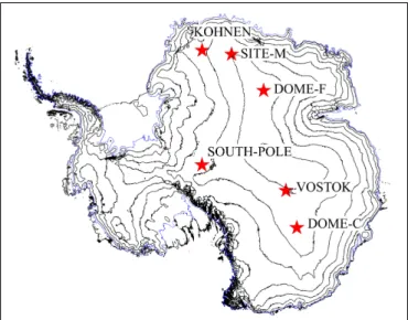
Kohnen Station is located in the Atlantic sector of the East Antarctic Plateau at 75◦000S 00◦040E (Figure 1). It lies 500 km off the coast at an elevation of 2892 m above sea level. The station was built as a summer station in 1998/99 during the European Project for Ice Coring in Antarctica (EPICA) and used as the logistic platform for the drilling of the deep ice core EDML (Drücker et al., 2002). Since it is situated about 10 km SW of an ice divide, the ice flows with low surface velocities of up to∼1 m per year (Wesche et al., 2007).
An automatic weather station (AWS 9) provides detailed information about the weather conditions at Kohnen since the late 90s, including 2-m air temperature, wind speed, and snow
FIGURE 1 |Map of Antarctica including our study area and other ice-core drilling sites for comparison; elevation model according toHowat et al. (2019).
height (Reijmer and Van Den Broeke, 2003;Helsen et al., 2005).
The summer 2-m air temperature varies between−16 and−36◦C with pronounced diurnal cycles of−10 to−15◦C, whereas winter temperature drops down to−70◦C. However, warm low-pressure air masses interrupt the cold winter period and give reason for air temperatures up to−30◦C. Generally, the region is characterized by light katabatic winds downslope the ice divide. These stable weather conditions are superimposed by near-coastal, synoptic developments that occasionally lead to strong wind events at Kohnen Station (Reijmer and Van Den Broeke, 2003). Wind speeds>10 m s−1are associated with snowdrift and occasionally followed by dune formation (Birnbaum et al., 2010).
The accumulation rate, derived from firn core records, averages to 62 kg m−2a−1 over the last two centuries (Oerter et al., 2000).Medley et al. (2018)have documented a continuous increase to ∼75 kg m−2a−1 over the last 50 years. Compared to other sites on the East Antarctic plateau (Figure 1), this is relatively high accumulation. For example, it is two to three times higher than at Site M (36–53 kg m−2a−1, Karlöf et al., 2005), Dome C (∼25 kg m−2a−1, Stenni et al., 2016), Dome Fuji (27.3 ± 1.5 kg m−2a−1, Kameda et al., 2008), or Vostok (20–24 kg m−2a−1,Ekaykin et al., 2002;Touzeau et al., 2016). On the other hand, the accumulation rate at Kohnen Station is below
∼100 kg m−2a−1, which Hoshina et al. (2016) have proposed as lower resolution limit of seasonal cycles in major-ion and δ18O profiles.
While the estimated accumulation rate is in the upper range found on the East Antarctic Plateau, the following studies indicate that processes related to low accumulation are highly relevant at Kohnen. Neighboring profiles of density and stable water isotopes are poorly correlated in the low-accumulation Kohnen area (Laepple et al., 2016; Münch et al., 2016).
Surface roughness ranges in the same order of magnitude as accumulation rate (Laepple et al., 2016), and intermittent (re-) deposition (Helsen et al., 2005) as well as sporadic formation of barchan dunes have been reported (Birnbaum et al., 2010;
Proksch et al., 2015). Further, Münch et al. (2017) showed in a trench study that the stable water isotopic record at Kohnen is decoupled from the local temperature, even after spatially averaging over several profiles.
In this study, we present a multi-parameter analysis of a top-3-m snow profile retrieved from Kohnen Station.
We compare sub-millimeter-resolved microstructure records of density, crusts, and structural anisotropy with discrete measurements of sulfate, sodium, andδ18O of the same profile as well as AWS 9 data. Our findings highlight the interplay of the (post-)deposition history of the snow and proxy signal formation at this low-accumulation site on the East Antarctic Plateau.
MATERIALS AND METHODS Snow Sampling
In January 2015 during the Austral summer season, a 50-m long and 3.4-m deep trench (T15-1) was excavated and sampled for temporal and spatial analysis of stable water isotopes (Münch et al., 2017). The trench T15-1 was located about 500 m southeast
of the EDML deep-drilling site. Snow sampling for the present study was performed in the undisturbed snowpack at the first sampling position (0 m) of T15-1, a few centimeters next to the sampling of Münch et al. (2017). To retrieve a 3-m profile of snowpack, three carbon-fiber tubes (liners) of 1 m length, 10 cm diameter, and 0.1 cm wall thickness were carefully pushed into the snow. After each push, we checked that snow surfaces inside and surrounding the liner were consistent to guarantee sampling without compression. The second and third meters were sampled on freshly prepared surfaces 10 cm laterally displaced to the former liner positions without vertical overlaps. Then, the snow- filled liners were cut out sideward from the trench wall. We sealed their top and bottom faces with plastic bags and stored them in isolated transport boxes. At the end of the summer field season, the frozen samples were shipped home, stored at
−28◦C and analyzed in the cold lab at AWI, Bremerhaven, in April–May 2016.
Core-Scale Microfocus X-Ray Computer Tomography
First, the snow filled liners are non-destructively analyzed by the means of a core-scale microfocus X-ray computer tomograph (ice-µCT). The device is specially designed for ice core applications and methodologically based on microfocus X-ray computer tomography (Freitag et al., 2013). It is placed in a radiation-protected walk-in cold lab at −14◦C so that no additional construction is needed to keep the sample frozen during the measurements. Main components of the ice-µCT are a 140 kV X-ray source, a rotation desk with a sample holder and a 20×40 cm detector unit operating in fourfold-binned mode with 1000×2000 pixels in this specific application. All components are mounted on movable axes placed on air bearings. Spindle positioning allows the control of lateral and vertical movements of source and detector with displacements of up to 1.1 m traverse path. To avoid damage and to hold the snow core vertically aligned on the sample stage, the snow is kept inside the liners.
Density
The 2D density profile is generated with the ice-µCT operating in fly-by-mode. Thereby, radioscopic images are continuously captured during a synchronous upward movement of X-ray source and detector from bottom to top along the vertical axis of the snow-liner. The recorded stack of ∼2000 images provides information on integrated X-ray attenuation over beam paths with different off-axis angles through the snow sample. We use only the centerlines and the two adjacent pixel lines from each image to generate an image composite.
It compiles the X-ray attenuation in horizontal layers with a vertical resolution of 110 µm. Aiming to transfer X-ray attenuation to density information, we measure the attenuation of pure ice blocks with defined dimensions at the start of every snow-scan (Freitag et al., 2013). The replicate calibration takes into account instability plus aging of the X-ray source and improves the accuracy of the density estimates. In fact, the averaged densities of the ice-µCT profiles differ only ± 5 kg m−3 from bulk densities based on weight and volume with the same uncertainty band. Since the first
0.1 m of the upper liner filled with drifting snow during trench sampling, this section is not representative for the microstructure record.
Structural Parameters
All structural parameters are derived from 3D-volume reconstructions of the snow liners. For this, we perform ice-µCT measurements in a helical scan mode especially developed for vertically aligned objects like snow or ice cores. Starting at the top of the sample, X-ray source and detector move downward in a stop-and-go mode while the sample rotates stepwise.
During conventional CT measurements, the sample rotates 360◦ before source and detector positions change. Comparing these 3D measurement set-ups, the helical mode avoids cone-beam artifacts leading to depth-dependent segmentation errors. For a full 3D reconstruction of one snow liner, a series of∼35,000 images is taken. Its spatial resolution is 57 µm in lateral and vertical direction. The reconstructed volume image is segmented in ice and air fraction using an Otsu-threshold after smoothing with a 3×3×3 median filter (Otsu, 1979). A comparison of the 3D and 1D density shows only slight deviations<10 kg m−3 for all available depth intervals and confirms the accuracy of image segmentation. Subsequently, 3D structural parameters are derived from a running volume window of 1000×1000 ×77 voxels, corresponding to 5.7 ×5.7×0.44 cm in size. After the measurement campaign, we realized that the oversized tube holder in the beamline had reduced image quality in the lower 0.2 m of each snow core. Thus, we excluded these depth intervals from the analysis.
Detection of Crusts
Crusts are thin layers of heavily sintered grains. They are one- tenth of a millimeter thick, which is of the order of the diameter of one grain. In principle, they are visible as density peaks in a density profile with 110µm vertical resolution. However, not all crusts lie perpendicular to the vertical axis and therefore are hard to detect as sharp spikes in the density profile. To account for their irregular shape, we additionally inspect the segmented 3D volume reconstructions. We visually check each layer for localized, dense ice clusters embedded in a regular pattern of the porous ice matrix. If such an anomaly extends in adjacent layers over the entire horizontal area, the feature is defined as a crust.
Mean Chord Length and Geometrical Anisotropy The mean chord length (MCL) of the ice matrix is defined as the mean over all intersections of an object within a volume along a certain direction. Here, we calculate the MCLs of the ice phase in two horizontal directions (MCLX, MCLY) and in vertical direction (MCLZ) within a running volume window of 5.7 ×5.7× 0.44 cm along the snow profile. The upper limits for MCLX,Y,Zare the window dimensions with the lowest bound of 0.44 cm in z-direction. All truncated chord lengths with direct contact to the border faces of the running window are not considered. Horizontal directions are arbitrary directions.
The calculated values are assigned to the mean depth of the running volume window. Note that CT reconstructions are not
able to resolve grain boundaries, and chord lengths are not strictly synonymous with grain or crystallite size dimensions (Freitag et al., 2008).
In this study, we define geometrical anisotropyaas a ratio between the horizontal and the vertical MCL. Thereby, we use the mean of MCLX and MCLY as the best estimate for the horizontal chord length. Then, geometric anisotropy a can be calculated using
a= MCLx+ MCLy 2×MCLz
A value of a = 1 means that the ice matrix of the snow is geometrical isotropic in horizontal and vertical direction. A value ofa >1 refers to a horizontally elongated ice matrix, a value ofa <1 points to a vertically elongated ice matrix. Vertically elongated structures are expected in snow affected by vertically oriented temperature-gradient metamorphism. We note that this calculation of anisotropy differs from previous studies (e.g.Löwe et al., 2013; Calonne et al., 2014), in which a is the vertical component over the horizontal one.
Discrete Measurements of Stable Water Isotopes and Trace Components
In order to measure impurities and isotopic composition, the core is cut into discrete samples at an interval of 1.1 cm. We stabilize the core segments in a stainless-steel trough and sequentially cut samples with a ceramic knife. While the knife transects the snow, we extract inner sample material by screwing in a bottle of 6.3 cm diameter. Due to the brevity of contact with ambient air, this inner part is considered uncontaminated. A range of ion concentrations is measured by means of ion chromatography (Thermo Fisher Scientific Co., ICS2100).
Here, we specifically focus on sodium and sulfate. Based on their concentrations, we compute the non-sea-salt sulfate (nss- SO42−
) fraction by subtracting the sea salt contribution from bulk sulfate concentration (Göktas et al., 2002).
[nss-SO42−] = [SO42−] −0.252× [Na+]
The outer part of the snow samples is analyzed regarding stable water isotopic composition by means of cavity ring- down spectroscopy (Gupta et al., 2009), using commercially available Picarro instruments. The data are calibrated against in-house standards and corrected for memory effects as well as drift during measurements (Van Geldern and Barth, 2012). The measurements are reported against the international standard of Vienna Standard Mean Ocean Water (V-SMOW). The precision is in the range of 0.1hforδ18O.
Temperature and Snow Height Data From AWS 9
We use the 2-m air temperature record of the weather station AWS 9, 500 m northwest of our sampling site, to derive daily temperatures and temperature gradients, i.e. the difference between daily temperature minimum and maximum. The snow height sensor record is analyzed for relative changes in the surface height. Thereby, a decreasing distance between the
sensor and the snow surface implies deposition. The annual change in height is fitted linearly and counted as cumulative deposition at the surface. In this study, we specifically assess the fraction of deposition over the summer season. In this regard, we define a narrow 4-month summer window from November to February and a broader 6-month summer period from September equinox to March equinox, respectively. Snow height changes within these intervals are hereafter referred to as summer deposition. In order to determine the expected summer deposition, we assume equally distributed deposition throughout the year, calculate the portion of total annual deposition for each month, and subsequently compute the four-fold and sixfold portion, respectively. Afterward, we compare observed changes in snow height during summer months to the expected summer deposition. If the observed fraction of deposition matches the expected deposition, the ratio equals 1. If less (more) deposition is observed than expected, the ratio is smaller (larger) than 1.
RESULTS
Physical Properties and Features of the Profile
Density
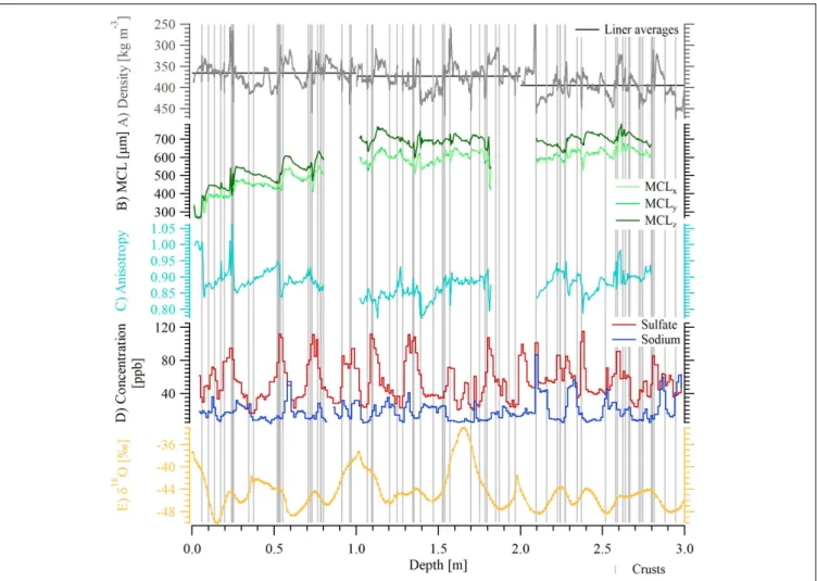
The density profile of the uppermost 3-m snowpack at Kohnen Station is characterized by strong variations (Figure 2A). Single values range between 250 and 450 kg m−3. The snowpack is composed of cm-thick layers, each displaying a specific density value. The differences in density between adjacent layers range between 50 and 100 kg m−3. The liner average density values rise from 366 kg m−3 (liner 1) to 394 kg m−3 (liner 3). This overall increase of 30 kg m−3 is smaller than the observed changes among adjacent layers, indicating that the compaction within the first 3 m is negligible in comparison to the inter-layer variations on a cm scale.
Crusts
Crusts are evident as sharp high-density peaks on a sub- millimeter scale (Figure 2A). In total, we counted 75 crusts in both the 1D and 3D reconstruction and indicate them as vertical lines inFigure 2. Extent and tilt of such crusts are visible in the 3D volume reconstruction (Figure 3). They often appear in close conjunction with thin layers of very low density. Approximately 40% of the detected crusts cluster in multi-crust sections, which appear localized in 10–12 horizons throughout the profile.
Layer Thickness
We find the cm-thick layers in the density record to be typically separated by crusts (Figure 2A). Therefore, we use crusts to separate single (density) layers and derive the thickness of the deposits. Our layer separation technique by the means of crusts is independent of absolute density values and avoids the arbitrary definition of thresholds as separation markers. The resulting frequency distribution of layer thickness, given as the distance between two adjacent crusts, is displayed on a logarithmic scale (Figure 4). The layer thickness distribution follows roughly a bimodal distribution, separating sections with multiple thin
crusts on the left-hand side from a thickness distribution of layers without intersecting crusts on the right-hand side (Figure 4).
Both distributions are fitted by Gaussian functions. A small contribution of extraordinary large layer thickness at the upper tail of the latter distribution is excluded from the Gaussian fits.
We interpret these few sections as layers not confined by crusts but differing levels of density. The layer thickness distributions for the multi-crust layers center at 0.8 cm and 68% of the layers range between 0.2 and 3 cm. For deposited layers with defined single crusts as borders, the median lies at 4 cm with 68% ranging between 2 and 9 cm. Since the local accumulation rate of 70–
80 kg m−2a−1equals∼20 cm of snow per year, the derived mean layer thickness of 4 cm snow implies that the snow at Kohnen Station is deposited during five to six events per year, i.e. the snow profile consists of event-based deposits like at 0.24–0.54 m depth (Figure 2A). However, we note that deposition is not equal to precipitation.
Mean Chord Lengths
The MCLs MCLX, MCLY, and MCLZ increase from ∼300 to
∼600µm in the uppermost meter (Figure 2B) and then remain approximately constant until 3 m depth. The record shows a recurring pattern of sharp increases in MCL followed by a steady decline, for example, at 0.24–0.54 m depth. In the following, we refer to this pattern as saw-tooth pattern. It is more pronounced in the vertical MCLZ than in the other two directions, with a mean offset of 75µm and the largest difference just after each sharp increase. In the uppermost meter, for example at 0.24–
0.54 m depth, this MCL pattern is by no means visible in the density data. In the third meter, however, one can observe a gradual increase in density in parallel with a decrease in MCL, e.g. at 2.28–2.50 m depth.
Anisotropy
The geometric anisotropy record of the ice matrix starts with values around 1, indicating isotropic snow at the surface (Figure 2C). Below, we find the saw-tooth pattern introduced by a varying difference between vertical and horizontal MCL values. The first saw tooth begins 0.1 m below the surface with an abrupt drop to 0.85, a moderate vertical anisotropy. This jump is followed by a smooth increase with depth, until it reaches values of ≥1 in a thin layer. The saw-tooth pattern is repeated three times within the first meter of the profile and recurs at 1.4–1.6 and 2.3–2.5 m depth (Figure 2C). Thereby, the vertical extent of the saw tooth ranges from 0.10 to 0.25 m, and minor substructures exist, for example, at 0.52–0.7 and 2.37–2.52 m depth. At 1.1–
1.4 and 1.6–1.8 m depth, the anisotropy stays at almost constant values. Apart from a thin layer at 0.23 m depth, the anisotropy values are<1 throughout the profile and result from vertically elongated structures of the ice matrix.
Chemical Properties of the Profile
Sulfate concentration varies periodically between a base level of nearly 40 ppb and peaks up to 115 ppb throughout the profile (Figure 2D). Between 14 and 17 peaks can be counted.
Most of them have a broad base, but some rise sharply or display double peaks. We find sulfate peaks linked with the sharp
FIGURE 2 |Microstructure, trace elements, and isotopic composition displayed against depth from the single snow profile near Kohnen Station.(A)Density retrieved from a 2D radioscopic scan composite, and liner averages, note the reversed axis.(B)Mean chord lengths alongx-,y-, andz-axis (MCLX, MCLY, MCLZ) of the ice phase based on a 3D volume scan, color code according to the legend.(C)Geometric anisotropy based on a 3D volume scan and derived from MCL.
(D)Total sulfate (red) and sodium (dark blue) concentrations from discrete measurements.(E)Stable water isotopicδ18O measured discretely; surface crust positions are indicated by light gray markers.
jumps in anisotropy and crust positions, for example, at 0.53 m depth. The nss-SO42− record closely resembles the behavior of bulk sulfate.
Sodium concentrations range between minimum 4 and 40 ppb. The mean concentration is 20 ppb (Figure 2D).
Intervals of minor and higher sodium concentration alternate continuously. Some sodium intervals like at 2.2 m depth are bounded by distinct concentration changes. The vertical extent of specific sodium concentration values tends to correlate with (density) layers as defined from the crust profile (Figures 2A,D).
For example, homogeneously elevated sodium concentrations at 1.4–1.54 m depth are abruptly taken over by a depleted sodium plateau at 1.54–1.71 m depth. These sodium signals correspond two intervals of increasing and decreasing density at the according depth.
The values of δ18O range between −50 and −33h with a mean of −44h (Figure 2E). We identify 12 ± 1 cycles in the snow profile. As displayed at 1.2–1.4 and 2.6–2.8 m depth, some of them are of small amplitude and occur as
double peaks. Prominent high and broad peaks exist around 1.0 and 1.7 m depth.
Air Temperatures and Summer Deposition
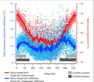
Based on mean daily temperatures measured over the period from the year 2000 to 2015, the average annual cycle ranges from −24◦C in summer to −50◦C in winter (Figure 5). Even temperatures down to −70◦C are common during winter.
Temperature differences between day and night in the range of 10–15◦C occur in spring and autumn, when the sun warms the air during daytime, but the low angle of the sun causes cold nights.
The annual snow height change averages 22.5 cm over the entire observation period 2000–2015. Thus, 7.5 cm snow and 11.25 cm snow are expected during the 4-month and 6-month summer season, respectively. However, the fraction of deposition derived from the snow height sensor reveals inhomogeneous deposition of snow during the summer months (Figures 6,7D).
FIGURE 3 |3D section of a crust at∼0.26 m depth; color code: white = ice, black = air.
FIGURE 4 |Bimodal Gaussian distribution of logarithmic layer thickness for the deposited layers of the snow profile near Kohnen Station; the mean layer thickness in multi-crust-clusters centers at 0.8 cm; layers confined by single crusts have an average thickness of 4 cm; sections separated by changes in density but without internal crusts lie at the top tail of the Gaussian distribution.
In the Austral summers 2005–2006, 2007–2008, and 2010–2011, more deposition than expected was recorded at the AWS 9. In other years, like 2002–2005, 2009–2010, or 2013–2015, the site experienced much less deposition or even erosion during the
FIGURE 5 |Daily air temperature measurements of the years 2000–2015 (red dots) derived from AWS 9 and averaged to obtain an average annual cycle (red thick line); the difference between daily minimum and maximum temperature was calculated accordingly (blue); gray bars indicate a narrow, 4-month and a broader, 6-month summer period for summer deposition evaluation below (see text), color code according to the legend.
FIGURE 6 |Summer deposition of the years 2000–2015 derived from the AWS 9 snow height sensor displayed against time; dashed lines indicate the expected summer deposition, bars show the observed summer deposition;
color code: light gray = 4-month summer period November–February, dark gray = 6-month summer period from September equinox to March equinox.
summer months. Assuming uniform deposition throughout the year, the 4-month summer period receives on average 52% and the 6-month summer half-year 74% of the deposition expected.
Though we note that the AWS snow height sensor is only a point measurement and lacks information about the spatial variability of deposition, it gives evidence for a trend of weaker summer deposition.
Dating
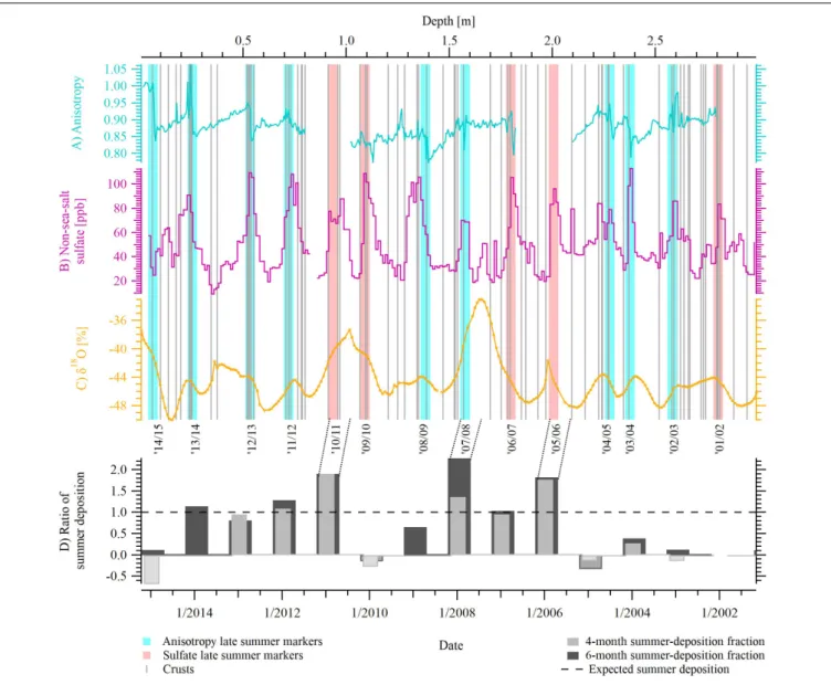
In order to date the snow profile, we combine nss-SO42− concentration and surface crust positions (Figure 7). We
FIGURE 7 |Comparison of(A)geometric anisotropy,(B)non-sea-salt sulfate, and(C)stable water isotoeδ18O; summer markers are based on seasonality in geometric anisotropy and completed using sulfate peaks;(D)ratio between expected and observed snow accumulation during the 4-month and 6-month summer period derived from AWS 9; color code according to legend.
interpret nss-SO42−peaks as a late summer-to-fall signal because atmospheric nss-SO42−concentration at Kohnen Station peaks in summer, January–February (Piel et al., 2006; Weller and Wagenbach, 2007), whereas elevated nss-SO42−
concentration in ice cores are markers of fall (Göktas et al., 2002). Following previous studies on the East Antarctic Plateau (Koerner, 1971;
Ren et al., 2004;Hoshina et al., 2014), density crusts were applied as summer markers, because strong solar insolation during this season fosters their formation. Based on the agreement of these two parameters, we identify 14–15 summer layers in our snow profile, and the snow profile covers the period from 2002 until 2015 (Figure 7). Comparing our dating approach with the anisotropy record, we find the jumps in anisotropy to coincide with summer-to-fall markers of crusts and nss-SO42− peaks throughout the profile (Figure 7).
DISCUSSION
Seasonal Anisotropy and Deposition
The observed co-variation of microstructural anisotropy with the peaks of nss-SO42− and crusts implies a seasonal pattern in the snow microstructure. Here, we discuss possible reasons and mechanisms for the repeated formation of microstructural anisotropy and its saw-tooth shape.
Previous studies have shown that vertical anisotropy in the snowpack results from temperature-gradient metamorphism (Srivastava et al., 2010; Calonne et al., 2017). The effective heat conductivity of snow results from several aspects such as structure, density, history of the snow pack, and applied temperature (Satyawali et al., 2008; Calonne et al., 2019). The latter varies on a daily and seasonal time scale as recorded by
the AWS (Figure 5). Accordingly, a macroscopic temperature gradient persists in the snow column (Picard et al., 2012;Pinzer et al., 2012; Calonne et al., 2014), which can be as high as 25–
50◦Cm−1 on a daily time scale. Such conditions are similar to gradients applied in laboratory experiments (Pfeffer and Mrugala, 2002; Riche et al., 2013), leading to a gradual formation of chain-like structures in vertical direction and depth hoar.
In order to explain the observed saw-tooth-shaped anisotropy profile, a snow layer must be exposed to a persistent temperature gradient over a certain period. Then, the impact of the gradient and the formation of anisotropy is strongest at the surface and penetrates deeper into the snowpack with decreasing strength (e.g. Colbeck, 1989; Picard et al., 2012; Calonne et al., 2014), leading to the observed gradual decrease with depth. Since we find surface crusts, formed by sun radiation and wind polishing in times of non-deposition (e.g. Gow, 1965; Koerner, 1971), clustered in depth intervals of strongest anisotropy, we suggest that, while the gradient is applied to the snowpack, no new deposition is added on top. The sharp drop in anisotropy, indicating an interruption of the previous temperature-gradient regime, could be a combination of decreased water vapor pressure, i.e. a temperature decrease toward the end of summer, and new snow on top.
With respect to the timing of the repeated anisotropy formation, we note that the intensity of metamorphism depends on both the ambient temperature and the diurnal gradient (Colbeck, 1989; Fukuzawa and Akitaya, 1991; Kamata et al., 1999). While absolute temperatures at Kohnen Station are highest during summer and enable larger water-vapor-pressure gradients in the snowpack, gradients are strongest during spring and autumn (Figure 5). Thus, anisotropic growth could occur from spring to autumn, depending on when the snow is exposed at the surface over a longer period. At the South Pole, anisotropic depth hoar has been designated as stratigraphic marker of late summer to autumn (Gow, 1965;Koerner, 1971).
Considering the overall warmer mean air temperatures during summer and the observed large gradients in the spring and autumn, the conditions favoring enhanced temperature-gradient metamorphism at Kohnen appear in the summer months.
The repetitive saw-tooth pattern in anisotropy indicates not only periodic conditions favoring metamorphism but points to the daily gradient as reason for anisotropy formation. A saw tooth with the observed, vertical extent of 0.1–0.25 m can result from the limited penetration depth of the daily gradient and solar radiation (Colbeck, 1989). Furthermore, the saw-tooth pattern imprinted at the surface would probably experience modification, if enhanced temperature-gradient metamorphism took place at greater depth due to a seasonal-induced gradient. However, we also find the pattern at depths of 1.4–1.6 and 2.3–2.5 m.
We hypothesize that the formation of the observed anisotropy pattern is related to inhomogeneous deposition in summer, i.e.
precipitation intermittency. Arguments are (a) the dating, where we find peak anisotropy to coincide with summer-to-fall peaks in nss-SO42− and clusters of crusts, (b) the combination of highest mean air temperatures and strong gradients favoring grain growth in summer to fall, and (c) the irregular summer deposition derived from AWS 9: We find sometimes very reduced
or even negative amount of deposition, i.e. erosion. On the other hand, we find years with higher-than-expected values of summer deposition, such as in the summers 2007/2008 and 2010/2011 (Figures 6,7D). In the snow profile, these years can be linked to depth intervals with homogenous anisotropy lacking a saw tooth, comparably highδ18O values, and lower nss-SO42− concentrations with multiple peaks (Figure 7D).
From AWS 9 data, we know that no or negative deposition over the entire summer is only an extreme case of the trend to weaker summer deposition. Considering the case of occasional summer deposition, the initial anisotropy of the surface snow is low but develops faster than the anisotropy of the overburden snow. Thus, summer snow can reach the same anisotropy values after a certain time of exposure. We note that, in order to generate a steady saw-tooth pattern over all summer snow layers, exposure time and strength of temperature-gradient metamorphism must be balanced. Otherwise, the anisotropy profile shows a more step-like, sub-structured behavior. Since our anisotropy profile exhibits minor substructures in the saw- tooth pattern at 0.52–0.72 and 2.37–2.52 m depth, it permits such an interpretation. Altogether, we propose that the development of a saw tooth points to phases of non-deposition, as the combined observation of microstructure, impurities, crusts, and AWS allows of such hypothesis.
Besides a formation during discontinuities in precipitation, the saw-tooth pattern in anisotropy can also develop in consequence of surface undulations. Wind-induced dune layers are exposed at the surface even after new snowfall fills up the intermediate troughs. Consequently, surface snow exposure to temperature gradients is prolonged and may generate a saw tooth in anisotropy. This additional formation factor cannot be neglected because dune formation is evident at Kohnen Station, and the spatial variability of accumulation on the East Antarctic plateau is large (Frezzotti et al., 2005;Fujita et al., 2011).
Implications for Chemical Proxies
Considering the discontinuous character of snow deposition at our site and the observed tendency for decreased summer deposition, we can evaluate not only the derived microstructure but also the impurity concentration profiles in the snowpack. We here do not intend to discuss fluxes of aerosols to the snow but discuss the deposition history of trace component concentrations and what we can learn about deposition mechanisms.
As sulfate peaks go along with surface crusts and jumps of anisotropy in this profile (Figures 2,7), sulfate and nss-SO42−
concentrations could be related to the deposition conditions at the end of summer. The peak found in the summer-to-fall transition is then related to the deposition of new snow after a deposition-free period, i.e. it cumulates in the new snow.
This could either indicate increased atmospheric concentrations during summer, which are just collected within the snow of the late summer-to-fall deposition, or it indicates a seasonal peak of sulfate in the fall rather than summer, which is directly displayed in the snow profile. At Dome Fuji, Iizuka et al. (2004) demonstrated non-sea-salt sulfate minima during summer and proposed a diurnal sublimation-condensation
mechanism as explanation. However, this mechanism has not been observed at Kohnen Station so far. To disclose the enrichment process of sulfate in the surface snow at Kohnen Station, a timely resolved analysis of the exact timing of the sulfate with respect to the microstructure is necessary.
However, its cannot be retrieved at this point due to the discrete, vertical sampling resolution of 1.1 cm, the ± 1 cm uncertainty in depth assignments, and the sub-millimeter dimensions of crusts.
Since plateaus with homogeneous sodium concentration record are frequently linked to the extent of (density) layers (Figure 2), we propose that specific (density) layers carry a specific chemical load. This load depends on their deposition in consequence of precipitation or wind-driven redistribution (Groot Zwaaftink et al., 2013;Hoshina et al., 2014). Combined analyses of density and sodium concentration could therefore help to distinguish whether a snow record displays a deposition history based on few-events-only or a continuous deposition throughout the year.
The stable water isotope record seems to be affected by the proposed precipitation intermittency (this snow profile, and Münch et al., 2017). For example, in the years 2003–2005, 2008–
2009, or 2009–2010 with little-to-no summer deposition, we find depletedδ18O signatures during summer. Complementary, we observe less depleted δ18O values in the years 2007–2008 and 2010–2011 with larger summer deposition, supporting the AWS-derived finding of more, warmer summer snow deposition in these years. Indeed, warm temperature periods during synoptic events are associated with increased amounts of precipitation (Helsen et al., 2005). This indicates that the retrieved stable water isotope record and the related annual mean values from Kohnen Station could be dominated by few deposition events.
Among other processes affecting the isotope records in East Antarctica (Neumann et al., 2005;Town et al., 2008; Hoshina et al., 2014;Ritter et al., 2016;Casado et al., 2018;Laepple et al., 2018), the here derived precipitation intermittency could partly explain the previously observed decoupling of δ18O from the annual mean air temperature record (Münch et al., 2017).
Comparison of Accumulation Rate and Precipitation Intermittency to Previous Studies
Comparing our findings to previous meteorological studies at Kohnen Station, our dating approach leads to 4–5 years per meter and confirms recent accumulation-rate estimates of 0.2–0.25 m of snow per year (Medley et al., 2018). In greater detail, Reijmer and Van Den Broeke (2003)stated that both small snowfall events of 1–2 cm thickness and synoptic precipitation >5 cm contribute to the annual accumulation at the site. Our bimodal distribution of layer thickness, centering at 0.8 and 4 cm, also suggests two modes of accumulation (Figure 4). With approximately five (density) layers per year, our microstructure profile resembles previous estimates of three to five synoptic snowfall events per year (Noone et al., 1999;
Birnbaum et al., 2006; Schlosser et al., 2010). However, the
number of layers could also originate from post-depositional redistribution. Synoptic snowfall conditions in conjunction with wind can lead to dune formation, and Birnbaum et al.
(2010) suggest an annual frequency of three to eight dune formation events of 4 ±2 cm each. For now, a discrimination between deposition of layers resulting from precipitation and layers resulting from wind-redistribution remains unclear in our density profile.
On the other hand, the expression of a precipitation or deposition intermittency in the Kohnen area, appearing in snow microstructure and proxy concentration variations measured in the snow, has not been documented yet. Previous studies of Reijmer and Van Den Broeke (2003) andHelsen et al. (2005) have discussed both against and for a seasonality of precipitation around the Kohnen Station, respectively. Thus, our seasonal interpretation of the repeated anisotropy saw-tooth remains controversial, even though it agrees with AWS data and field observations of S. Kipfstuhl throughout the last 15 years.
Comparison to Other Sites
In this study, we applied the combination of non-sea-salt sulfate, typically used at high-accumulation sites (Minikin et al., 1998), and surface crusts, previously used at low- accumulation sites like the South Pole (Gow, 1965; Koerner, 1971), to date the snow profile. In contrast to findings of Hoshina et al. (2014) at Dome Fuji, the crust record at Kohnen Station alone is not unambiguous, but multi-crust layers are concentrated in depth intervals of large non- sea-salt sulfate and anisotropy (Figure 7). This illustrates that Kohnen Station is not typical for the East Antarctic Plateau, but that its annual accumulation rate at the upper end of the low-accumulation range allows for distinct snow characteristics (Hoshina et al., 2016). Transferring our interpretation of anisotropy to other sites on the East Antarctic Plateau is challenging because most of them receive even less accumulation than Kohnen Station, and the temporal and spatial variability of precipitation is large (Ekaykin et al., 2002; Kameda et al., 2008; Stenni et al., 2016). Longer exposure times at the surface could amplify the impact of temperature-gradient metamorphism at other sites. However, anisotropic structures may be readily destroyed, if snow deposits persistently undergo wind redistribution. Whether microstructural anisotropy develops and is preserved under various environmental conditions on the East Antarctic Plateau needs site-specific investigation.
CONCLUSION
With this study, we aim to give insight into the deposition history of the East Antarctic snowpack near Kohnen Station and to better understand the processes shaping climate proxy records in ice cores from sites with low to moderate accumulation rates. Therefore, we have performed combined measurements of microstructure, trace elements, and stable water isotopes on a 3-m snow core retrieved at Kohnen Station and
used meteorological data from AWS 9. A very prominent feature of the microstructure profile is the recurring saw-tooth pattern in geometric anisotropy formed by (daily) temperature- gradient metamorphism. Combining the microstructural record with chemical and meteorological information, we draw the following conclusions: (1) the anisotropy saw- tooth develops seasonally and confirms a summer-to-fall dating approach based on nss-SO42−
concentration and clusters of surface crusts at Kohnen Station; (2) snow microstructure indicates deposition intermittency with an underrepresentation of summer snow, which is supported by snow height measurements of the automatic weather station; and (3) summer deposition intermittency strongly affects the interpretation of climate proxy parameters: it determines the recording of sulfate and sodium in the snow deposits in various ways, and stable water isotopes show a systematic bias toward the winter season or interannual variations decoupled from climatic changes. After all, this multi-parameter study discloses a yearly resolved record instead of a solely layered snowpack. To elaborate the site- specific potential of snow-microstructure information for the interpretation of climate proxy records at other East Antarctic sites, further investigations in low-accumulation areas will be necessary. The quantification of deposition hiatus based on microstructure would be of particular interest because years of missing snow are difficult to judge so far.
DATA AVAILABILITY STATEMENT
δ18O, trace element profiles and the derived microstructure data will be made available in the PANGAEA data library. Raw CT data of this article will be made available by the authors to any qualified researcher. Requests to access the datasets should be directed to JF.
AUTHOR CONTRIBUTIONS
SK, JF, MH, and DM conceptualized the study. DM and JF conducted the ice-µCT measurements. DM, JF, and MH contributed to the interpretation of the results and wrote the first draft of the manuscript. All authors contributed to the manuscript revision and read and approved the submitted version.
ACKNOWLEDGMENTS
We thank the reviewers for their constructive comments, which have improved our manuscript substantially. We also thank C.
Reijmer for providing daily data from AWS 9, which is operated by the University of Utrecht. Furthermore, we want to thank B. Twarloh, T. Bluszcz, and Y. Schlomann for conducting the measurements on stable water isotopes and ion concentrations.
REFERENCES
Alley, R. B. (1988). Concerning the deposition and diagenesis of strata in polar firn.
J. Glaciol.34, 283–290. doi: 10.3189/S0022143000007024
Birnbaum, G., Brauner, R., and Ries, H. (2006). Synoptic situations causing high precipitation rates on the antarctic plateau: observations from Kohnen Station, Dronning Maud Land. Antarct. Sci. 18, 279–288. doi: 10.1017/
S0954102006000320
Birnbaum, G., Freitag, J., Brauner, R., König-Langlo, G., Schulz, E., Kipfstuhl, S., et al. (2010). Strong-wind events and their influence on the formation of snow dunes: observations from Kohnen station, Dronning Maud Land, Antarctica.
J. Glaciol.56, 891–902. doi: 10.3189/002214310794457272
Brook, E. J., and Buizert, C. (2018). Antarctic and global climate history viewed from ice cores.Nature558, 200–208. doi: 10.1038/s41586-018-0172-175 Brun, E., Six, D., Picard, G., Vionnet, V., Arnaud, L., Bazile, E., et al. (2011).
Snow/atmosphere coupled simulation at Dome C, Antarctica.J. Glaciol.57, 721–736. doi: 10.3189/002214311797409794
Calonne, N., Flin, F., Geindreau, C., Lesaffre, B., and Rolland Du Roscoat, S. (2014).
Study of a temperature gradient metamorphism of snow from 3-D images:
time evolution of microstructures, physical properties and their associated anisotropy.Cryosphere8, 2255–2274. doi: 10.5194/tc-8-2255-2014
Calonne, N., Milliancourt, L., Burr, A., Philip, A., Martin, C. L., Flin, F., et al. (2019). Thermal conductivity of snow, firn, and porous ice from 3-D image-based computations.Geophys. Res. Lett.46, 13079–13089. doi: 10.1029/
2019GL085228
Calonne, N., Montagnat, M., Matzl, M., and Schneebeli, M. (2017). The layered evolution of fabric and microstructure of snow at point Barnola, Central East Antarctica.Earth Planet. Sci. Lett.460, 293–301. doi: 10.1016/j.epsl.2016.11.041 Carlsen, T., Birnbaum, G., Ehrlich, A., Freitag, J., Heygster, G., Istomina, L., et al.
(2017). Comparison of different methods to retrieve optical-equivalent snow grain size in central Antarctica.Cryosphere11, 2727–2741. doi: 10.5194/tc-11- 2727-2017
Casado, M., Landais, A., Picard, G., Münch, T., Laepple, T., Stenni, B., et al. (2018).
Archival processes of the water stable isotope signal in East Antarctic ice cores.
Cryosphere12, 1745–1766. doi: 10.5194/tc-12-1745-2018
Colbeck, S. C. (1989). Snow-crystal growth with varying surface temperatures and radiation penetration.J. Glaciol.35, 23–29. doi: 10.3189/002214389793701536 Courville, Z. R., Albert, M. R., Fahnestock, M. A., Cathles, I. M., and Shuman,
C. A. (2007). Impacts of an accumulation hiatus on the physical properties of firn at a low-accumulation polar site.J. Geophys. Res. Earth Surf.112, 1–11.
doi: 10.1029/2005JF000429
Drücker, C., Wilhelms, F., Oerter, H., Frenzel, A., Gernandt, H., and Miller, H. (2002). “Design, transport, construction, and operation of the summer base Kohnen for ice-core drilling in Dronning Maud Land, Antarctica,” in Proceedings of the Fifth International Workshop on Ice Drilling Technology (Nagaoka: Nagaoka University of Technology), 302–312.
Ekaykin, A. A., Lipenkov, V. Y., Barkov, N. I., Petit, J. R., and Masson-Delmotte, V.
(2002). Spatial and temporal variability in isotope composition of recent snow in the vicinity of Vostok station, Antarctica: implications for ice-core record interpretation.Ann. Glaciol.35, 181–186. doi: 10.3189/172756402781816726 EPICA Community Members (2006). One-to-one coupling of glacial climate
variability in greenland and Antarctica.Nature444, 195–198. doi: 10.1038/
nature05301
Fegyveresi, J. M., Alley, R. B., Muto, A., Orsi, A. J., and Spencer, M. K. (2018).
Surface formation, preservation, and history of low-porosity crusts at the WAIS Divide site, West Antarctica.Cryosphere12, 325–341. doi: 10.5194/tc-12-325- 2018
Freitag, J., Kipfstuhl, S., and Faria, S. H. (2008). The connectivity of crystallite agglomerates in low-density firn at Kohnen station, Dronning Maud Land, Antarctica.Ann. Glaciol.49, 114–119. doi: 10.3189/172756408787814852 Freitag, J., Kipfstuhl, S., and Laepple, T. (2013). Core-scale radioscopic imaging:
a new method reveals density-calcium link in Antarctic firn.J. Glaciol.59, 1009–1014. doi: 10.3189/2013JoG13J028
Frezzotti, M., Pourchet, M., Flora, O., Gandolfi, S., Gay, M., Urbini, S., et al. (2005).
Spatial and temporal variability of snow accumulation in East Antarctica from traverse data.J. Glaciol.51, 113–124. doi: 10.3189/172756505781829502 Fujita, S., Holmlund, P., Andersson, I., Brown, I., Enomoto, H., Fujii, Y., et al.
(2011). Spatial and temporal variability of snow accumulation rate on the East Antarctic ice divide between Dome Fuji and EPICA DML.Cryosphere5, 1057–1081. doi: 10.5194/tc-5-1057-2011
Fukuzawa, T., and Akitaya, E. (1991). An experimental study on the growth rates of depth hoar crystals at high temperature gradients (I).Low Temp. Sci. Ser. A 50, 9–14.
Furukawa, R., Uemura, R., Fujita, K., Sjolte, J., Yoshimura, K., Matoba, S., et al.
(2017). Seasonal-scale dating of a shallow ice core from greenland using oxygen isotope matching between data and simulation.J. Geophys. Res. Atmos.122, 10873–10887. doi: 10.1002/2017JD026716
Göktas, F., Fischer, H., Oerter, H., Weller, R., Sommer, S., Miller, H., et al. (2002).
A glaciochemical characterization of the new EPICA deep-drilling site on Amundsen-isen, dronning Maud Land, Antarctica.Ann. Glaciol.35, 347–354.
doi: 10.3189/172756402781816474
Gow, A. J. (1965). On the accumulation and seasonal stratification of snow at the South Pole.J. Glaciol.5, 467–477. doi: 10.1017/S002214300001844X Groot Zwaaftink, C. D., Cagnati, A., Crepaz, A., Fierz, C., MacElloni, G., Valt,
M., et al. (2013). Event-driven deposition of snow on the Antarctic Plateau:
analyzing field measurements with snowpack.Cryosphere7, 333–347. doi: 10.
5194/tc-7-333-2013
Gupta, P., Noone, D., Galewsky, J., Sweeney, C., and Vaughn, B. H. (2009).
Demonstration of high-precision continuous measurements of water vapor isotopologues in laboratory and remote field deployments using wavelength- scanned cavity ring-down spectroscopy (WS-CRDS) technology. Rapid Commun. Mass Spectrom.23, 2534–2542. doi: 10.1002/rcm.4100
Helsen, M. M., Van de Wal, R. S. W., Van Den Broeke, M. R., As, D., Va1eijer, H. A. J., and Reijmer, C. H. (2005). Oxygen isotope variability in snow from western dronning Maud Land, Antarctica and its relation to temperature.Tellus B Chem. Phys. Meteorol.57, 423–435. doi: 10.3402/tellusb.v57i5.16563 Hörhold, M. W., Albert, M. R., and Freitag, J. (2009). The impact of accumulation
rate on anisotropy and air permeability of polar firn at a high-accumulation site.
J. Glaciol.55, 625–630. doi: 10.3189/002214309789471021
Hoshina, Y., Fujita, K., Iizuka, Y., and Motoyama, H. (2016). Inconsistent relationships between major ions and water stable isotopes in Antarctic snow under different accumulation environments.Polar Sci.10, 1–10. doi: 10.1016/j.
polar.2015.12.003
Hoshina, Y., Fujita, K., Nakazawa, F., Iizuka, Y., Miyake, T., Hirabayashi, M., et al.
(2014). Effect of accumulation rate on water stable isotopes of near-surface snow in inland Antarctica.J. Geophys. Res.119, 274–283. doi: 10.1002/2013JD020771 Howat, I. M., Porter, C., Smith, B. E., Noh, M.-J., and Morin, P. (2019). The reference elevation model of Antarctica.Cryosphere13, 665–674. doi: 10.5194/
tc-13-665-2019
Iizuka, Y., Fujii, Y., Hirasawa, N., Suzuki, T., Motoyama, H., Furukawa, T., et al.
(2004). SO2-4 minimum in summer snow layer at Dome Fuji, Antarctica, and the probable mechanism.J. Geophys. Res. Atmos.109:4138. doi: 10.1029/
2003jd004138
Iizuka, Y., Ohno, H., Uemura, R., Suzuki, T., Oyabu, I., Hoshina, Y., et al. (2016).
Spatial distributions of soluble salts in surface snow of East Antarctica.Tellus Ser. B Chem. Phys. Meteorol.68:29285. doi: 10.3402/tellusb.v68.29285 Johnsen, S. J. (1977). “Stable isotope homogenization of polar firn and ice,”
in Proceedings of Symposium on Isotopes and Impurities in Snow and Ice, International Association of Hydrological Sciences, Commission of Snow and Ice, I.U.G.G. XVI, Wallingford.
Jonsell, U., Hansson, M. E., and Mörth, C. M. (2007). Correlations between concentrations of acids and oxygen isotope ratios in polar surface snow.Tellus Ser. B Chem. Phys. Meteorol.59, 326–335. doi: 10.1111/j.1600-0889.2007.00272.
x
Jouzel, J., Alley, R. B., Cuffey, K. M., Dansgaard, W., Grootes, P., Hoffmann, G., et al. (1997). Validity of the temperature reconstruction from water isotopes in ice cores.J. Geophys. Res. Ocean.102, 26471–26487. doi: 10.1029/97JC01283 Jouzel, J., Masson-Delmotte, V., Cattani, O., Dreyfus, G., Falourd, S., Hoffmann,
G., et al. (2007). Orbital and millennial antarctic climate variability over the past 800,000 years.Science317, 793–796. doi: 10.1126/science.1141038 Kamata, Y., Sokratov, S. A., and Sato, A. (1999). “Temperature and temperature
gradient dependence of snow recrystallization in depth hoar snow,” inAdvances in Cold-Region Thermal Engineering and Sciences, eds K. Hutter, Y. Wang, and H. Beer ((Heidelberg: Springer), 395–402. doi: 10.1007/bfb0104197
Kameda, T., Motoyama, H., Fujita, S., and Takahashi, S. (2008). Temporal and spatial variability of surface mass balance at Dome Fuji, East Antarctica, by the stake method from 1995 to 2006.J. Glaciol.54, 107–115. doi: 10.3189/
002214308784409062
Karlöf, L., Isaksson, E., Winther, J.-G., Gundestrup, N., Meijer, H. A. J., Mulvaney, R., et al. (2005). Accumulation variability over a small area in east Dronning Maud Land, Antarctica, as determined from shallow firn cores and snow pits:
some implications for ice-core records.J. Glaciol.51, 343–352. doi: 10.3189/
172756505781829232
Kaufmann, P., Fundel, F., Fischer, H., Bigler, M., Ruth, U., Udisti, R., et al. (2010).
Ammonium and non-sea salt sulfate in the EPICA ice cores as indicator of biological activity in the Southern Ocean.Quat. Sci. Rev.29, 313–323. doi:
10.1016/j.quascirev.2009.11.009
Koerner, R. M. (1971). A stratigraphic method of determining the snow accumulation rate at plateau station, Antarctica, and application to south pole- queen maud land traverse 2, 1965-1966.Antarct. Ice Stud.2, 225–238. doi:
10.1029/AR016p0225
Laepple, T., Hörhold, M., Münch, T., Freitag, J., Wegner, A., and Kipfstuhl, S.
(2016). Layering of surface snow and firn at Kohnen Station, Antarctica: noise or seasonal signal?J. Geophys. Res. Earth Surf.121, 1849–1860. doi: 10.1002/
2016JF003919
Laepple, T., Münch, T., Casado, M., Hoerhold, M., Landais, A., and Kipfstuhl, S. (2018). On the similarity and apparent cycles of isotopic variations in East Antarctic snow pits.Cryosphere12, 169–187. doi: 10.5194/tc-12-169-2018 Legrand, M. (1995). Sulphur-derived species in polar ice: a review.Ice Core Stud.
Glob. Biogeochem. Cycles30, 91–119. doi: 10.1007/978-3-642-51172-1-5 Legrand, M., and Mayewski, P. (1997). Glaciochemistry of polar ice cores: a review.
Rev. Geophys.35, 219–243. doi: 10.1029/96RG03527
Löwe, H., Riche, F., and Schneebeli, M. (2013). A general treatment of snow microstructure exemplified by an improved relation for thermal conductivity.
Cryosphere7, 1473–1480. doi: 10.5194/tc-7-1473-2013
Lüthi, D., Le Floch, M., Bereiter, B., Blunier, T., Barnola, J. M., Siegenthaler, U., et al.
(2008). High-resolution carbon dioxide concentration record 650,000-800,000 years before present.Nature453, 379–382. doi: 10.1038/nature06949 Masson-Delmotte, V., Hou, S., Ekaykin, A., Jouzel, J., Aristarain, A., Bernardo,
R. T., et al. (2008). A review of antarctic surface snow isotopic composition:
observations, atmospheric circulation, and isotopic modeling. J. Clim.21, 3359–3387. doi: 10.1175/2007JCLI2139.1
Medley, B., McConnell, J. R., Neumann, T. A., Reijmer, C. H., Chellman, N., Sigl, M., et al. (2018). Temperature and snowfall in western queen maud land increasing faster than climate model projections.Geophys. Res. Lett.45, 1472–1480. doi: 10.1002/2017GL075992
Minikin, A., Legrand, M., Hall, J., Wagenbach, D., Kleefeld, C., Wolff, E., et al.
(1998). Sulfur-containing species (sulfate and methanesulfonate) in coastal Antarctic aerosol and precipitation.J. Geophys. Res. Atmos.103, 10975–10990.
doi: 10.1029/98JD00249
Mosley-Thompson, E., Kruss, P. D., Thompson, L. G., Pourchet, M., and Grootes, P. (1985). Snow stratigraphic record at South pole: potential for paleoclimatic reconstruction.Ann. Glaciol.7, 26–33. doi: 10.3189/S0260305500005863 Münch, T., Kipfstuhl, S., Freitag, J., Meyer, H., and Laepple, T. (2016). Regional
climate signal vs. local noise: a two-dimensional view of water isotopes in Antarctic firn at Kohnen Station, Dronning Maud Land.Clim. Past12, 1565–
1581. doi: 10.5194/cp-12-1565-2016
Münch, T., Kipfstuhl, S., Freitag, J., Meyer, H., and Laepple, T. (2017). Constraints on post-depositional isotope modifications in East Antarctic firn from analysing temporal changes of isotope profiles.Cryosphere11, 2175–2188. doi: 10.5194/
tc-11-2175-2017
Münch, T., and Laepple, T. (2018). What climate signal is contained in decadal- to centennial-scale isotope variations from Antarctic ice cores?Clim. Past14, 2053–2070. doi: 10.5194/cp-14-2053-2018
Neumann, T. A., Waddington, E. D., Steig, E. J., and Grootes, P. M. (2005). Non- climate influences on stable isotopes at Taylor Mouth, Antarctica.J. Glaciol.51, 248–258. doi: 10.3189/172756505781829331
Noone, D., Turner, J., and Mulvaney, R. (1999). Atmospheric signals and characteristics of accumulation in dronning Maud Land, Antarctica.J. Geophys.
Res. Atmos.104, 19191–19211. doi: 10.1029/1999JD900376
Oerter, H., Wilhelms, F., Jung-Rothenhausler, F., Goktas, F., Miller, H., Graf, W., et al. (2000). Accumulation rates in Dronning Maud Land, Antarctica, as revealed by dielectric-profiling measurements of shallow firn cores.Ann.
Glaciol.30, 27–34. doi: 10.3189/172756400781820705
Otsu, N. (1979). A threshold selection method from gray-level histograms.IEEE Trans. Syst. Man. Cybern.9, 62–66. doi: 10.1109/TSMC.1979.4310076