SFB 649 Discussion Paper 2014-065
A Theory of Price
Adjustment under Loss Aversion
Steffen Ahrens*
Inske Pirschel**
Dennis J. Snower***
* Technische Universität Berlin, Germany
** Kiel Institute for the World Economy, Germany
***Christian-Albrechts University, Germany
This research was supported by the Deutsche
Forschungsgemeinschaft through the SFB 649 "Economic Risk".
http://sfb649.wiwi.hu-berlin.de ISSN 1860-5664
SFB 649, Humboldt-Universität zu Berlin
S FB
6 4 9
E C O N O M I C
R I S K
B E R L I N
A Theory of Price Adjustment under Loss Aversion ∗
Steffen Ahrens
a,b, Inske Pirschel
b,c, and Dennis J. Snower
b,c,daTechnische Universität Berlin, Straße des 17. Juni 135, 10623 Berlin, Germany
bKiel Institute for the World Economy, Kiellinie 66, 24105 Kiel, Germany
cChristian-Albrechts University, Kiel, Wilhem-Seelig-Platz 1, 24118 Kiel, Germany
dCEPR and IZA
October 30, 2014
Abstract
We present a new partial equilibrium theory of price adjustment, based on con- sumer loss aversion. In line with prospect theory, the consumers’ perceived utility losses from price increases are weighted more heavily than the perceived utility gains from price decreases of equal magnitude. Price changes are evaluated rel- ative to an endogenous reference price, which depends on the consumers’ ratio- nal price expectations from the recent past. By implication, demand responses are more elastic for price increases than for price decreases and thus firms face a downward-sloping demand curve that is kinked at the consumers’ reference price.
Firms adjust their prices flexibly in response to variations in this demand curve, in the context of an otherwise standard dynamic neoclassical model of monopolistic competition. The resulting theory of price adjustment is starkly at variance with past theories. We find that - in line with the empirical evidence - prices are more sluggish upwards than downwards in response to temporary demand shocks, while they are more sluggish downwards than upwards in response to permanent demand shocks.
JEL classification: D03, D21, E31, E50.
Keywords: price sluggishness, loss aversion, state-dependent pricing
∗This paper is part of the Kiel-INET research group on new economic thinking. We thank the participants at the 18th Spring Meeting of Young Economists 2013 in Aarhus (Denmark), the 2013 Annual Meeting of the German Economic Association in Düsseldorf (Germany), and the Scottish Economic Society Annual Conference 2014 in Perth (Scotland) for fruitful discussions. Steffen Ahrens acknowledges support by the Deutsche Forschungsgemeinschaft (DFG) through the CRC 649 “Economic Risk.”
E-mail: steffen.ahrens@tu-berlin.de (S. Ahrens), inske.pirschel@ifw-kiel.de (I. Pirschel),
dennis.snower@ifw-kiel.de (D.J. Snower).
1 Introduction
This paper presents a theory of price sluggishness based on consumer loss aversion, along the lines of prospect theory (Kahnemann and Tversky, 1979). The theory has distinctive implications, which are starkly at variance with major existing theories of price adjustment. In particular, the theory implies that prices are more sluggish up- wards than downwards in response to temporary demand shocks, while they are more sluggish downwards than upwards in response to permanent demand shocks.
These implications turn out to be consonant with recent empirical evidence. Though this evidence has not thus far attracted much explicit attention, it is clearly implicit in a range of influential empirical results. For instance, Hall et al. (2000) document that firms mostly accommodate negative temporary demand shifts by temporary price cuts, yet they are reluctant to temporarily increase their prices in response to positive tem- porary demand shifts. Furthermore, the empirical evidence provided by Kehoe and Midrigan (2008) indicates that temporary price reductions are - on average - larger and much more frequent than temporary price increases, implying that prices are relatively downward responsive.
By contrast, in the event of a permanent demand shock, the empirical evidence points towards a stronger upward flexibility of prices for a wide variety of industrialized countries (Kandil, 1995, 1996, 1998, 2001, 2002a,b 2010; Weise, 1999; Karras 1996;
Karras and Stokes 1999) as well as developing countries (Kandil, 1998).
While current theories of price adjustment (e.g. Taylor, 1979; Rotemberg, 1982;
Calvo, 1983; among many others) fail to account for these empirical regularities, this paper offers a possible theoretical rationale.
The basic idea underlying our theory is simple. Price increases are associated with utility losses for consumers, whereas price decreases are associated with utility gains.
In the spirit of prospect theory, losses are weighted more heavily than gains of equal magnitude. Consequently, demand responses are more elastic to price increases than to price decreases. The result is a kinked demand curve1, for which the kink depends on the consumers’ reference price. In the spirit of K˝oszegi and Rabin (2006), we model the reference price as the consumers’ rational price expectations. We assume that con- sumers know, with a one period lag, whether any given demand shock is temporary or permanent. Permanent shocks induce changes in the consumers’ rational price expec- tations and thereby in their reference price, while temporary shocks do not.
Given the demand shock is temporary, the kink of the demand curve implies that sufficiently small shocks do not affect the firm’s price. This is the case of price rigidity.
For larger shocks, the firm’s price will respond temporarily, but the size of the response will be asymmetric for positive and negative shifts of equal magnitude. Since negative shocks move the firm along the relatively steep portion of the demand curve, prices decline stronger to negative shocks than they increase to equiproportionate positive shocks.
By contrast, given the demand shock is permanent, the firm can foresee not only the change in demand following its immediate pricing decision, but also the resulting change in the consumers’ reference price. A rise in the reference price raises the firms’
long-run profits (since the reference price is located at the kink of the demand curve),
1Modeling price sluggishness by means of a kinked demand curve is of course a well-trodden path.
Sweezy (1939) and Hall and Hitch (1939) modeled price rigidity in an oligopolistic framework along these lines. In these models, oligopolistic firms do not change their prices flexibly because of their expected asymmetric competitor’s reactions to their pricing decisions. A game theoretic foundation of such model is presented by Maskin and Tirole (1988).
whereas a fall in the reference price lowers long-run profits, a phenomenon which we term the reference-price updating effect. On this account, firms are averse to initiating permanent price reductions. By implication, prices are more sluggish downwards than upwards for permanent demand shocks.
These results are extremely important for the conduct of monetary policy, since they imply that the sign of the asymmetry of price adjustment depends on the per- sistence of the underlying demand shock. In particular, if temporary demand shocks are interpreted as non-persistent and permanent demand shocks as fully persistent, our analysis implies that there exists a balance point (i.e. an intermediate degree of per- sistence of the shock) at which the asymmetry reverses. For shocks less persistent than the balance point prices are more sluggish upwards than downwards, while they are more sluggish downwards than upwards for more persistent shocks. Whether the degree of persistence at the balance point is relatively high or low depends on the ad- justment speed of the reference price and on the firm’s discount factor. An increase in the adjustment speed of the reference price, as well as in the firm’s discount factor, strengthens the role of the reference-price updating effect, increasing upward flexibility and downward sluggishness at any given positive persistence of the shock. Therefore, the balance point will be associated with a lower level of persistence. To the best of our knowledge, there is no other paper studying the ramifications of the persistence of the demand shock for asymmetric price adjustment.
The paper is structured as follows. Section 2 reviews the relevant literature. Section 3 presents our general model setup and in Section 4 we analyze the effects of various demand shocks on prices, both analytically and numerically. Section 5 concludes.
2 Relation to the Literature
We now consider the empirical evidence suggesting that prices respond imperfectly and asymmetrically to exogenous positive and negative shocks of equal magnitude, and that the implied asymmetry depends on whether the shock is permanent or temporary.
There is much empirical evidence for the proposition that, with regard to perma- nent demand shocks, prices are generally more responsive to positive shocks than to negative ones. For example, in the context of monetary policy shocks, Kandil (1996, 2002b), Kandil (1995), and Weise (1999) find support for the United States over a large range of different samples. Moreover, Kandil (1995) and Karras and Stokes (1999) sup- ply evidence for large panels of industrialized OECD countries, while Karras (1996) provides evidence for developing countries. In the case of the United States, Kandil (2001, 2002a) shows that the asymmetry also prevails in response to permanent gov- ernment spending shocks. Kandil (1999, 2006, 2010), on the other hand, looks directly at permanent aggregate demand shocks and also confirms the asymmetry for a large set of industrialized countries as well as for a sample of disaggregated industries in the United States. Comparing a large set of industrialized and developing countries, Kandil (1998) finds that the asymmetry is even stronger for many developing countries compared to industrialized ones.
In addition to the asymmetric price reaction in response to permanent demand shocks, the above studies also find an asymmetric reaction of output. They show that output responds significantly less to permanent positive demand shocks relative to neg- ative ones. This asymmetry – which is also predicted by our model (as shown below) – is further documented by a large body of empirical literature that explicitly focuses on output. For example, DeLong and Summers (1988), Cover (1992), Thoma (1994), and
Ravn and Sola (2004) show for the United States that positive changes in the rate of money growth induce much weaker output reductions than negative changes in the rate of money supply. Morgan (1993) and Ravn and Sola (2004) confirm this asymmetry, when monetary policy is conducted via changes in the federal funds rate. Additional evidence is provided by Tan et al. (2010) for Indonesia, Malaysia, the Philippines, and Thailand and by Mehrara and Karsalari (2011) for Iran.
There is also significant empirical evidence for the proposition that, with regard to temporary demand shocks, prices are generally less responsive to positive shocks than to negative ones. For example, the survey by Hall et al. (2000) indicates that firms re- gard price increases as response to temporary increases in demand to be among the least favorable options. Instead, firms rather employ more workers, extend overtime work, or increase capacities. By contrast, managers of firms state that a temporary fall in demand is much more likely to lead to a price cut. Further evidence for the asymmetry in response to temporary demand shocks is provided by Kehoe and Midrigan (2008), who analyze temporary price movements at Dominick’s Finer Foods retail chain with weekly store-level data from 86 stores in the Chicago area. They find that temporary price reductions are much more frequent than temporary price increases and that, on average, temporary price cuts are larger (by a factor of almost two) than temporary price increases. However neither of these studies empirically analyzes the asymmetry characteristics of the output reaction in the face of temporary demand shocks.
Despite this broad evidence, asymmetric reactions to demand shocks have been unexplored by current theories of price adjustment. Neither time-dependent pricing models (Taylor, 1979; Calvo, 1983), nor state-dependent adjustment cost models of (S,s)type (e.g., Sheshinski and Weiss, 1977; Rotemberg, 1982; Caplin and Spulber, 1987; Caballero and Engel, 1993, 2007; Golosov and Lucas, 2007; Gertler and Leahy, 2008; Dotsey et al., 2009; Midrigan, 2011) are able to account for the asymmetry properties in price dynamics in response to positive and negative exogenous temporary and permanent shifts in demand.2
In this paper we offer a new theory of firm price setting resting on consumer loss aversion in an otherwise standard model of monopolistic competition. The resulting theory provides a novel rationale for the above empirical evidence on asymmetric price sluggishness. Although there is no hard evidence for a direct link from consumer loss aversion to price sluggishness, to the best of our knowledge, there is ample evidence that firms do not adjust their prices flexibly in order to avoid harming their customer relationships (see, e.g., Fabiani et al. (2006) for a survey of euro area countries, Blinder et al. (1998) for the United States3, and Hall et al. (2000) for the United Kingdom).4
Furthermore, there is extensive empirical evidence that customers are indeed loss averse in prices. Kalwani et al. (1990), Mayhew and Winer (1992), Krishnamurthi et al.
(1992), Putler (1992), Hardie et al. (1993), Kalyanaram and Little (1994), Raman and
2Once trend inflation is considered, menu costs can generally explain that prices are more downward sluggish than upwards (Ball and Mankiw, 1994). By contrast, our model does not rely on the assumption of trend inflation.
3In their survey, Blinder et al. (1998) additionally find clear evidence that the pricing of those firms for which the fear of antagonizing their customers through price changes plays an important role is relatively upward sluggish. Unfortunately, the authors do no distinguish between temporary and permanent shifts in demand in their survey questions.
4Further evidence for OECD countries is provided by, for example, Fabiani et al. (2004) for Italy, Loupias and Ricart (2004) for France, Zbaracki et al. (2004) for the United States, Alvarez and Hernando (2005) for Spain, Amirault et al. (2005) for Canada, Aucremanne and Druant (2005) for Belgium, Stahl (2005) for Ger- many, Lünnemann and Mathä (2006) for Luxembourg, Langbraaten et al. (2008) for Norway, Hoeberichts and Stokman (2010) for the Netherlands, Kwapil et al. (2010) for Austria, Martins (2010) for Portugal, Ólafsson et al. (2011) for Iceland, and Greenslade and Parker (2012) for the United Kingdom.
Bass (2002), Dossche et al. (2010), and many others find evidence for consumer loss aversion with respect to many different product categories available in supermarkets.
Furthermore, loss aversion in prices is also well documented in diverse activities such as restaurant visits (Morgan, 2008), vacation trips (Nicolau, 2008), real estate trade (Genesove and Mayer, 2001), phone calls (Bidwell et al., 1995), and energy use (Griffin and Schulman, 2005; Adeyemi and Hunt, 2007; Ryan and Plourde, 2007).
In our model, loss-averse consumers evaluate prices relative to a reference price.
K˝oszegi and Rabin (2006, 2007, 2009) and Heidhues and K˝oszegi (2005, 2008, 2014) argue that reference points are determined by agents’ rational expectations about out- comes from the recent past. There is much empirical evidence suggesting that reference points are determined by expectations, in concrete situations such as in police perfor- mance after final offer arbitration (Mas, 2006), in the United States TV show "Deal or no Deal" (Post et al., 2008), with respect to domestic violence (Card and Dahl, 2011), in cab drivers’ labor supply decisions (Crawford and Meng, 2011), or in the effort choices of professional golf players (Pope and Schweitzer, 2011). In the con- text of laboratory experiments, Knetsch and Wong (2009) and Marzilli Ericson and Fuster (2011) find supporting evidence from exchange experiments and Abeler et al.
(2011) do so through an effort provision experiment. Endogenizing consumers’ refer- ence prices in this way allows our model to capture that current price changes influence the consumers’ future reference price and thereby affect the demand functions via what we call the "reference-price updating effect." This effect rests on the observation that firms tend to increase the demand for their product by raising their consumers’ refer- ence price through, for example, setting a "suggested retail price" that is higher than the price actually charged (Thaler, 1985; Putler, 1992). These pieces of evidence are consonant with the assumptions underlying our analysis. Our analysis works out the implications of these assumptions for state-dependent price sluggishness in the form of asymmetric price adjustment for temporary and permanent demand shocks.
There are only a few other papers that study the implications of consumer loss aversion on firms’ pricing decisions. In an early account of price rigidity in response to demand and cost shocks has been presented by Sibly (2002, 2007). In a static environ- ment, Sibly (2002, 2007) shows that a monopolist may not change prices if she faces loss averse consumers with fixed, exogenously given reference prices. In their partic- ularly insightful contributions, Heidhues and K˝oszegi (2008) and Spiegler (2012) ana- lyze static monopolistic pricing decisions to cost and demand shocks under the assump- tion that the reference price is determined as a consumer’s recent rational expectations personal equilibrium in the spirit of K˝oszegi and Rabin (2006). Spiegler (2012) shows that incentives for price rigidity are even stronger for demand shocks compared to cost shocks. We follow Heidhues and K˝oszegi (2008) and Spiegler (2012) and assume en- dogenous rational expectations reference price formation, but, by contrast, consider a dynamic approach to the pricing decision of a monopolistically competitive firm facing loss averse consumers. Our dynamic approach confirms earlier findings that consumer loss aversion engenders price rigidity and allows us to study the asymmetry charac- teristics of pricing reactions to temporary and permanent demand shocks of different sign. Another study close to ours is Popescu and Wu (2007); although they analyze optimal pricing strategies in repeated market interactions with loss averse consumers and endogenous reference prices, they do not analyze the model’s reaction to demand shocks.
Finally, this paper offers a new microfounded rationale for state-dependent pricing.
The importance of state-dependence for firms’ pricing decisions is well documented.
For instance, in the countries of the euro area (Fabiani et al., 2006; Nicolitsas, 2013),
Scandinavia (Apel et al., 2005; Langbraaten et al., 2008; Ólafsson et al., 2011), the United States (Blinder et al., 1998), and Turkey ( ¸Sahinöz and Saraço˘glu, 2008), ap- proximately two third of the firms’ pricing decisions are indeed driven by the current state of the environment.5Menu costs, by contrast, are clearly rejected as a significant driver for deferred price adjustments in each of the empirical studies above.
3 Model
We incorporate reference-dependent preferences and loss aversion into an otherwise standard model of monopolistic competition. Consumers are price takers and loss averse with respect to prices. They evaluate prices relative to their reference prices, which depend on their rational price expectations. Prices higher than the reference price are associated with utility losses, while prices lower than the reference price are associated with utility gains. Losses are weighted more heavily than gains of equal magnitude. Firms are monopolistic competitors, supplying non-durable differentiated goods. Firms can change their prices freely in each period to maximize their profits.
3.1 Consumers
We follow Sibly (2007) and assume that the representative consumer’s period-utility Ut depends positively on the consumption of n imperfectly substitutable nondurable goodsqi,t withi∈(1, . . . ,n)and negatively on the "loss-aversion ratio"(pi,t/ri,t), i.e.
the ratio of the pricepi,tof goodito the consumer’s respective reference priceri,tof the good. The loss-aversion ratio, which describes how the phenomenon of loss aversion enters the utility function, may be rationalized in terms of (i) Thaler’s transaction utility (whereby the total utility that the consumer derives from a good is in part determined by how the consumer evaluates the quality of the financial terms of the acquisition of the good (Thaler, 1991)), (ii) Okun’s implicit firm-customer contracts (whereby firms and customers implicitly agree on fair and stable prices despite fluctuations in demand (Okun, 1981)), or (iii) Rotemberg’s customer anger or regret (Rotemberg 2005, 2010).
Further approaches that describe reference-dependence in the consumer’s utility func- tion in terms of a ratio of actual prices to references prices are McDonald and Sibly (2001, 2005) in the context of loss aversion with respect to wages and Sibly (1996, 2002) in the context of loss aversion with respect to prices and quality.6
The consumer’s preferences in period t are represented by the following utility function:
Ut(q1,t, ...,qn,t) =
"
n
∑
i=1pi,t ri,t
−µ
qi,t
!ρ#ρ1
, (1)
where 0<ρ <1 denotes the degree of substitutability between the different goods.
The parameterµis an indicator function of the form µ=
Γ for pi,t<ri,t, i.e. gain domain
∆ for pi,t>ri,t, i.e. loss domain , (2)
5However in the United Kingdom (Hall et al., 2000) and Canada (Amirault et al., 2004) state-dependence seems to be somewhat less important for firms’ pricing decision.
6Other examples in which prices directly enter the utility function are, for instance, Rosenkranz (2003) and Rosenkranz and Schmitz (2007) in the context of auctions and Popescu and Wu (2007), Nasiry and Popescu (2011), and Zhou (2011) in the context of customer loss aversion.
which describes the degree of the consumer’s loss aversion. For loss averse consumers,
∆>Γ, i.e. the utility losses from price increases are larger than the utility gains from price decreases of equal magnitude. The consumer’s reference priceri,t is formed at the beginning of each period. In the spirit of K˝oszegi and Rabin (2006), we assume that the consumer’s reference price depends on her lagged rational price expectation.
Demand shocks, which may or may not trigger price adjustment, materialize unexpect- edly in the course of the period and therefore do not enter the information set used by the consumer at the beginning of the period to form the reference price. Therefore, there is no instantaneous reaction of the reference price in the shock period even if the firm immediately adjusts its price in response to the shock. At the beginning of the next period, however, consumers update their infomation set and adjust their price ex- pectation accordingly (since they can now infer about the nature of the demand shock and the corresponding price change). While temporary price changes do not provoke a change in the consumer’s reference price7, the reference price changes in the period af- ter the occurrence of a permanent shock. Thus the consumer’s reference price is given byri,t=E[pi,t|It−1]. The consumer’s budget constraint is given by
n
∑
i=1pi,tqi,t=PtYt, (3) whereYtdenotes the consumer’s real income in periodt which is assumed to be con- stant andPtis the aggregate price index. For simplicity, we abstract from saving. This implies that consumers are completely myopic.8 In each period the consumer max- imizes her period-utility function (1) with respect to her budget constraint (3). The result is the consumer’s periodtdemand for the differentiated goodiwhich is given by
qi,t(pi,t,ri,t,µ) =Ptη pi,t
ri,t
−µ(η−1)
Yt
pηi,t, (4)
where η= 1−ρ1 denotes the elasticity of substitution between the different product varieties. The aggregate price indexPtis given by
Pt=
n
∑
i=1
pi,t
, pi,t
ri,t
−µ!1−η
1 1−η
. (5)
We assume that the number of firmsnis sufficiently large so that the pricing decision of a single firm does not affect the aggregate price index. Definingλ=η(1+µ)−µ, we can simplify equation (4) to
qi,t(pi,t,ri,t,λ) =rλi,t−ηp−λi,t PtηYt, (6) where the parameterλdenotes the price elasticity of demand, which depends onµand therefore takes different values for losses and gains. To simplify notation, we define
λ=
γ for pi,t<ri,t
δ for pi,t>ri,t , (7)
7Support for this assumption can be found in the example of sales, i.e. promotions, characterized by non- permanent price decreases, used by firms to temporarily increase consumers’ demand for their product (see e.g. Eichenbaum et al., 2011). Sales do not affect the consumers’ reference price. Otherwise firms would not conduct sales because any downward adjustment of the consumer’s reference price reduces long-run profits for the firm.
8Evidence to support this assumption is provided by Elmaghraby and Keskinocak (2003) who show that many purchase decisions of non-durable goods take place in economic environments which are characterized by myopic consumers.
withδ=η(1+∆)−∆>γ=η(1+Γ)−Γ. Equation (6) indicates that the consumer’s demand function for goodiis kinked at the reference priceri,t. The kink, lying at the intersection of the two demand curves qi,t(pi,t,ri,t,γ)andqi,t(pi,t,ri,t,δ), is given by the price-quantity combination
(pci,t,qci,t) =
ri,t,ri,t−ηPtηYt
, (8)
where "b" denotes the value of a variable at the kink. Changes in the reference price ri,tgive rise to a change of the position of the kink and also shift the demand curve as a whole. The direction of this shift depends on the sign of the differenceλ−η. We restrict our analysis toλ ≥η, i.e. we assume that an increase in the reference price shifts the demand curve outwards and vice versa.9
Needless to say, abstracting from reference-dependence and loss aversion in the consumer’s preferences represented by utility function (1), restores the standard text- book consumer demand function for a differentiated goodi, given by
qi,t(pi,t) =p−ηi,t PtηYt. (9) In what follows, we will use this standard model as a benchmark case, against which we compare the pricing decisions of a monopolistic competitive firm facing loss averse consumers.
3.2 Monopolistic Firms
Firms seek to maximize the discounted stream of current and future profits, taking into account the implications of their current pricing decision for the costumers’ reference price. For simplicity, we assume a two period time horizon. (This can serve as a rough approximation for forms of short-sightedness, such as hyperbolic discounting, when the first-period discount rate exceeds the second-period one.10)
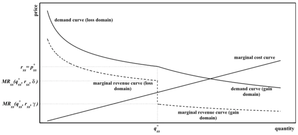
Allnfirms are identical, enabling us to drop the subscripti. In what follows we assume that the firm’s total costs are given byCt(qt) = c2qt2, where cis a constant, implying that marginal costs are linear in output:MCt(qt) =cqt. In the presence of loss aversion (δ>γ), the downward-sloping demand curve has a concave kink at the current reference price: pbt=rt. Thus the firm’s marginal revenue curve is discontinuous at the kink:
MRt(qt,rt,λ) =
1−1 λ
qt rt(λ−η)PtηYt
!−1
λ
, (10)
9The positive relationship between reference price and demand has become a common feature in the marketing sciences (e.g., Thaler, 1985; Putler, 1992; Greenleaf, 1995). It manifests itself, e.g., through the
"suggested retail price," by which raising the consumers’ reference price causes increases in demand (Thaler, 1985). Furthermore, Putler (1992) provides evidence that an extensive use of promotional pricing in the late 80’s had lead to an erosion in demand by lowering consumers’ reference prices.
10Many authors have shown that consumers’ discount rates are generally much higher in the short run than in the long run (e.g. Loewenstein and Thaler, 1989; Ainslie, 1992; Loewenstein and Prelec, 1992;
Laibson, 1996, 1997). Firm behavior is also often found to be short-sighted for the same reason. The theory of managerial myopia argues that managers often almost exclusively focus on short-term earnings (either because they have to meet certain goals or because their career advancement and compensation structure depends on the firm’s current performance), even if this has adverse long-run effects (Jacobson and Aaker, 1993; Graham et al., 2005; Mizik and Jacobson, 2007; Mizik, 2010). For a review of the early literature refer to Grant et al. (1996).
price
quantity qss∗
rss= pss∗
marginal revenue curve (gain domain)
demand curve (gain domain) marginal cost curve
marginal revenue curve (loss domain) demand curve (loss domain)
MRss(qss∗, rss, γ ) MRss(qss∗, rss, δ )
Figure 1: Initial steady state
withλ =γ for the gain domain and λ =δ for the loss domain, respectively. The interval[MRt(qbt,rt,γ), MRt(qbt,rt,δ)], whereMRt(qbt,rt,γ)<MRt(qbt,rt,δ), we call
“marginal revenue discontinuity”MRDt(qbt,rt,γ,δ).
We assume that in the initial steady state, the exogenously given reference price is rss. Furthermore, in the steady state the firm’s marginal cost curve intersects the marginal revenue discontinuity, as depicted in Figure 1. To fix ideas, we assume that initially the marginal cost curve crosses the midpoint of the discontinuity in the marginal revenue curve.11 This assumption permits us to derive the symmetry charac- teristics of the responses to positive and negative demand shocks. This implies that the firm’s optimal price in the initial steady statep∗ssis equal torss.12
4 Demand Shocks
The demand for each productiis subject to exogenous shocks, which may be temporary or permanent. These demand shocks, represented byεt, are unexpected and enter the demand function multiplicatively:
qt(pt,rt,λ,εt) =rt(λ−η)p−λt PtηYtεt. (11) The corresponding marginal revenue functions of the firm are
MRt(qt,rt,λ,εt) =
1−1 λ
qt
rt(λ−η)PtηYtεt
!−1
λ
. (12)
We consider the effects of a demand shock that hits the economy in period t=0.
The demand shock shifts the marginal revenue curve, along with the marginal revenue
11To satisfy this condition, the slope parametercof the marginal cost curve has to take the valuec=
1
2qss[MRt(qss,rss,γ) +MRt(qss,rss,δ)]
12The proof is straightforward: Letνbe an arbitrarily small number. Then for prices equal torss+νthe firm faces a situation in which marginal revenue is higher than marginal costs and decreasing the price would raise the firm’s profit, while for prices equal torss−νthe firm faces a situation in which marginal revenue is lower than marginal costs and increasing the price would raise the firm’s profit. Thusp∗ss=rsshas to be the profit maximizing price in the initial steady state.
discontinuityMRDt(qbt,rt,γ,δ,εt). We define a "small" shock as one that leaves the marginal cost curve passing through the marginal revenue discontinuity, and a "large"
shock as one that shifts the marginal revenue curve sufficiently so that the marginal cost curve no longer passes through the marginal revenue discontinuity.
The maximum size of a small shock for the demand function (11) is εt(λ) =
1−1
λ r1+ηt
cPtηYt
, (13)
i.e.εt(λ)is the shock size for which the marginal cost curve lies exactly on the bound- aries of the shifted marginal revenue discontinuityMRDt(qbt,rt,γ,δ,εt(λ)).13 In the analysis that follows, we will distinguish both between small and large demand shocks and between temporary and permanent demand shocks.
4.1 Temporary Demand Shocks
For a temporary (one-period) demand shock, the consumers’ reference price is not af- fected (since information reaches them with a one-period lag and they have rational expectations). Thus the firm’s price response to the shock is the same as that of a my- opic firm (which maximizes its current period profit).
Proposition 1:In response to a small temporary shock, prices remain rigid.
As noted, for a sufficiently small demand shockε0s≤ε0(λ)the marginal cost curve still intersects the marginal revenue discontinuity, i.e.MC0(qb0)∈MRD0 qb0,rss,γ,δ,ε0s
. Therefore, the prevailing steady state price remains the firm’s profit-maximizing price,14 i.e. p∗0=p∗ss, and we have complete price rigidity. By contrast, the profit-maximizing quantity changes toq∗0=r−ηss P0ηY0ε0s, thus the change of quantity is given by
∆q∗0= q∗0 q∗ss = ε0s
εss
=ε0s6=1. (14)
This holds true irrespective of the sign of the small temporary demand shock.
Proposition 2: In response to a large temporary shock, prices are more sluggish up- wards than downwards.
For a large shock, i.e.ε0l >ε0(λ), the marginal cost curve intersects the marginal revenue curve outside the discontinuity of the latter. Consequently both, a price and a quantity reaction are induced. The new profit-maximizing price of the firm is
p∗0= r(λ−η)ss P0ηY0ε0l q∗0
!λ1
, (15)
while its corresponding profit-maximizing quantity is q∗0=
1 c
1−1
λ λ+1λ
rss(λ−η)P0ηY0ε0l λ+11
, (16)
13Forε(δ), the marginal cost curve intersects the marginal revenue gap on the upper bound, whereas for ε(γ)it intersects it on the lower bound.
14Compare the proof from Section 3.2.
whereλ =δ for positive andλ=γfor negative shocks, respectively.
In comparison to the standard firm the price reaction of the firm facing loss-averse consumers in response to a large temporary demand shock is always smaller, whereas the quantity reaction is always larger. Additionally, prices and quantities are less re- sponsive to positive than to negative shocks. The intuition is obvious once we decom- pose the demand shock into the maximum small shock and the remainder:
ε0l =ε0(λ) +ε0rem. (17) From our theoretical analysis above, the maximum small shockε0(λ)has no price effects, but feeds one-to-one into demand. This holds true irrespective of the sign of the shock. By contrast, the remaining shockε0remhas asymmetric effects. Letq0be the quantity corresponding toε0(λ). Then the change in quantity in response toε0rem is given by
∆qrem0 =q∗0 q0=
ε0rem ε0(λ)
1 λ+1
. (18)
As can be seen from equation 18, the change of quantity in response toε0rem de- pends negatively onλ, the price elasticity of demand. Since by definitionδ >γ, the quantity reaction of the firm facing loss-averse consumers is smaller in response to large positive temporary demand shocks than to large negative ones. This however im- plies that prices are also less responsive to positive than to negative large temporary demand shocks, because the former move the firm along the relatively flat portion of the demand curve, whereas the latter move it along the relatively steep portion of the demand curve. This asymmetric sluggishness in the reaction to positive and negative large temporary demand shocks is a distinct feature of consumer loss aversion and stands in obvious contrast to the standard textbook case of monopoly pricing.
4.2 Permanent Demand Shocks
Now consider a permanent, demand shock that occurs in periodt=0. Whereas the firm is assumed to change its price immediately in response to this shock, consumers update their reference price in the following periodt=1, i.e.r1=E0[p1]. Consequently, for price increases (decreases) the demand curve shifts outwards (inwards) and the kink moves to
(pb1,qb1) = r1,(P1/r1)ηY1ε1
. (19)
An outward shift of the demand curve (initiated by an upward adjustment in the refer- ence price) increases the firm’s long-run profits, whereas an inward shift (initiated by a downward adjustment of the reference price) lowers them. We term this phenomenon the “reference-price updating effect.” The firm can anticipate this. Thus, it may have an incentive to set its price above the level that maximizes its profits in the shock period p00>p∗0, therewith exploiting (dampening) the outward (inward) shift of the demand curve resulting from the upward (downward) adjustment of the consumers’
reference price for positive (negative) permanent shocks.15 Whether this occurs de- pends on whether the firm’s gain from a price rise relative to p∗0in terms of future
15Needless to say, setting a price lower than optimal in the shock period with the aim to decrease the reference price permanently is not a preferable option for the firm.
Parameter Symbol Value
Discount rate β 0.99
Elasticity of substitution η 5 implying substitutability ρ 0.8 Price elasticity (gain domain) γ 6 Price elasticity (loss domain) δ 12
Loss aversion κ 2
Exogenous nominal income Y 1
Exogenous price index Pt 1
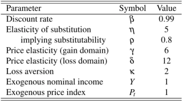
Table 1: Base calibration
profits (Π1(r1=p00)>Π1(r1=p∗0), due to the relative rise in the reference price) ex- ceeds the firm’s loss in terms of present profits (Π0(p00)<Π0(p∗0), since the pricep00 is not appropriate for maximizing current profit).
To analyze which effect dominates, we calibrate the model and solve it numerically.
4.3 Calibration
We calibrate the model for a quarterly frequency in accordance with standard values in the literature. We assume an annual interest rate of 4 percent, which yields a discount factorβ=0.99. We follow Schmitt-Grohé and Uribe (2007) and set the monopolistic markup to 25 percent, i.e.η=5, which is also close to the value supported by Erceg et al. (2000) and which implies that goods are only little substitutable, i.e.ρ=0.8. Since we imposeλ≥η, we setγ=6 in our base calibration. Loss aversion is measured by the relative slopes of the demand curves in the gain and loss domain, i.e. κ=δ
γ. The empirical literature on loss aversion in prices finds that losses induce demand reactions approximately twice as large as gains (Tversky and Kahnemann, 1991; Putler, 1992;
Hardie et al., 1993; Griffin and Schulman, 2005; Adeyemi and Hunt, 2007). Therefore, we setκ=2. The exogenous nominal incomeY and price indexPtare normalized to unity.16The base calibration is summarized in Table 1.
4.4 Numerical Simulation
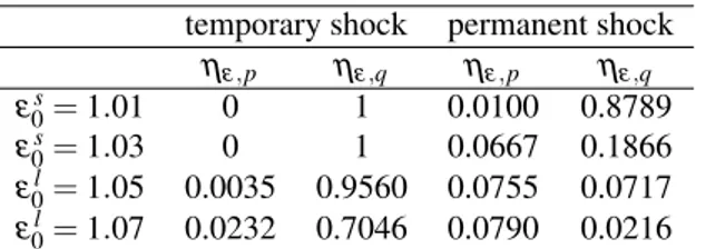
Tables 2 and 3 present the numerical results of our base calibration in the two-period model. In the tables we report the shock-arc-elasticities of price
ηeε,p=%∆p%∆ε and output
ηeε,q=%∆q%∆ε
in the period of the shockt=0 for positive and negative tempo- rary and permanent shocks for the firm facing loss averse consumers.
The results in Tables 2 and 3 confirm the theoretical analysis above for the tempo- rary shock, summarized in Propositions 1 and 2. However, not all of these results carry over in the case of permanent demand shocks.
Proposition 3:For all permanent shocks, prices are less sluggish upwards than down- wards.
In line with the theoretical analysis above, our numerical results in table 2 and 3 indicate that in the case of a permanent shock the firm exploits the "reference-price up-
16All results are completely robust to variations of these numerical values.
temporary shock permanent shock ηε,p ηε,q ηε,p ηε,q
ε0s=1.01 0 1 0.0100 0.8789
ε0s=1.03 0 1 0.0667 0.1866
ε0l=1.05 0.0035 0.9560 0.0755 0.0717 ε0l=1.07 0.0232 0.7046 0.0790 0.0216
Table 2: Shock elasticities of price and output int=0 to positive permanent demand shocks,ε0(γ) =1.0476
temporary shock permanent shock ηε,p ηε,q ηε,p ηε,q
ε0s=0.99 0 1 0 1
ε0s=0.97 0 1 0 1
ε0l=0.95 0.0072 0.9592 0.0012 0.9934 ε0l=0.93 0.0484 0.7264 0.0013 0.9927
Table 3: Shock elasticities of price and output int=0 to negative permanent demand shocks;ε0(δ) =0.9524
dating effect" and generally sets a price that is higher than the price it would optimally set in response to a temporary shock, i.e. p00>p∗0. For positive permanent demand shocks this implies that the pricing reaction of the firm is always stronger than for positive temporary demand shocks for both, small17 and large shocks18. By contrast, for negative permanent demand shocks firms either do not adjust their prices at all for sufficiently small shocks or to a considerably lower extent than for negative temporary shocks.
As a consequence, price sluggishness is considerably less pronounced for positive than for negative permanent demand shocks. The asymmetry of the price reaction to positive and negative shocks therefore reverses, when moving from temporary to permanent shocks. While this result may seem surprising at first glance, it is straight- forward intuitively: As noted, for temporary shocks, consumers abstract from updating their reference price. Therefore, the firm does not risk to suffer from a downward ad- justment of the consumers’ reference price, when encountering a temporary drop in demand with a price reduction. On the other hand, for positive temporary shocks, the firm cannot generate permanent increases in demand due to upward-adjustments of the reference price. Since consumers react more sensitive to price increases relative to price decreases, the price and quantity reactions are smaller for positive temporary shocks compared to negative ones. By contrast, for permanent demand shocks, the firm ex- ploits the positive "reference-price updating effect" which follows from price increases in response to positive shocks, whereas it tries to avoid the negative "reference-price updating effect" which follows from price decrease in response to negative shocks.19
17Of course, one can find a range of shocks, which are small enough to induce full price rigidity for permanent positive shocks. Due to the reference-price updating effect, this threshold is, however, very small.
Given the base calibration, the threshold value for a sufficiently small positive shock isε0(δ) =1.0087.
18Our numerical analysis indicates, however, that the positive reference-price updating effect is never strong enough to invalidate the general result that the pricing reaction of the firm facing loss averse consumers is more sluggish compared to the standard firm.
19Since the firm avoids price reductions, which lead to downward-adjustments in the reference price, but
5 Conclusion
In contrast to the standard time-dependent and state-dependent models of price slug- gishness, our theory of price adjustment is able to account for asymmetric price and quantity responses to positive and negative temporary and permanent shocks of equal magnitude. In contrast to the New Keynesian literature, our explanation of price adjust- ment is thoroughly microfounded, without recourse to ad hoc assumptions concerning the frequency of price changes or physical costs of price adjustments.
There are many avenues of future research. Consideration of heterogeneous firms and multi-product firms will enable this model to generate asynchronous price changes, as well as the simultaneous occurrence of large and small price changes, and heteroge- neous frequency of price changes across products. Extending the model to a stochastic environment will generate testable implications concerning the variability of individ- ual prices. Furthermore, our model needs to be incorporated into a general equilibrium setting to validate the predictions of our theory.
6 References
Abeler, J., A. Falk, L. Goette, and D. Huffman (2011). Reference points and effort provision. American Economic Review 101(2), 470-492.
Adeyemi, O.I. and L.C. Hunt (2007). Modelling OECD industrial energy demand:
Asymmetric price responses and energy-saving technical change. Energy Economics 29(4), 693-709.
Ainslie, G.W. (1992). Picoeconomics. Cambridge: Cambridge University Press.
Alvarez, L.J. and I. Hernando (2005). The price setting behavior of Spanish firms: Ev- idence from survey data. Working Paper Series 0538, European Central Bank.
Amirault, D., C. Kwan, and G. Wilkinson (2005). Survey of price-setting behaviour of Canadian companies. Bank of Canada Review - Winter 2004-2005, 29-40.
Apel, M., R. Friberg, and K. Hallsten (2005). Microfoundations of macroeconomic price adjustment: Survey evidence from Swedish firms. Journal of Money, Credit and Banking 37(2), 313-338.
Aucremanne, L. and M. Druant (2005). Price-setting behaviour in Belgium: What can be learned from an ad hoc survey? Working Paper Series 0448, European Central Bank.
Ball, L. and N.G. Mankiw (1994). Asymmetric price adjustment and economic fluctu- ations. Economic Journal 104(423), 247-261.
Bidwell, M.O., B.R. Wang, and J.D. Zona (1995). An analysis of asymmetric demand response to price changes: The case of local telephone calls. Journal of Regulatory Economics 8(3), 285-298.
conducts price reductions, which do not influence the reference price, loss aversion offers a simple rationale for the firm’s practice of “sales”(see e.g. Eichenbaum et al., 2011).
Blinder, A., E.R.D. Canetti, D.E. Lebow, and J.B. Rudd (1998). Asking about prices:
A new approach to understanding price stickiness. New York: Russel Sage Foundation.
Caballero, R.J. and E.M.R.A. Engel (1993). Heterogeneity and output fluctuations in a dynamic menu-cost economy. Review of Economic Studies 60(1), 95-119.
Caballero, R.J. and E.M.R.A. Engel (2007). Price stickiness in Ss models: New inter- pretations of old results. Journal of Monetary Economics 54(Supplement), 100-121.
Calvo, G.A. (1983). Staggered prices in a utility-maximizing framework. Journal of Monetary Economics 12(3), 383-398.
Caplin, A.S. and D.F. Spulber (1987). Menu costs and the neutrality of money. The Quarterly Journal of Economics 102(4), 703-725.
Card, D. and G.B. Dahl (2011). Family violence and football: The effect of unexpected emotional cues on violent behavior. The Quarterly Journal of Economics 126(1), 103- 143.
Cover, J.P. (1992). Asymmetric effects of positive and negative money-supply shocks.
The Quarterly Journal of Economics 107(4), 1261-1282.
Crawford, V.P. and J. Meng (2011). New York City cab drivers’ labor supply revisited:
Reference-dependent preferences with rational-expectations targets for hours and in- come. American Economic Review 101(5), 1912-1932.
DeLong, J.B. and L.H. Summers (1988). How does macroeconomic policy affect out- put? Brookings Papers on Economic Activity 19(2), 433-494.
Dixit, A.K. and J.E. Stiglitz (1977). Monopolistic competition and optimum product diversity. American Economic Review 67(3), 297-308.
Dossche, M., F. Heylen, and D. Van den Poel (2010). The kinked demand curve and price rigidity: Evidence from scanner data. Scandinavian Journal of Economics 112(4), 723-752.
Dotsey, M., R.G. King, and A.L. Wolman (2009). Inflation and real activity with firm level productivity shocks. 2009 Meeting Papers 367, Society for Economic Dynamics.
Eichenbaum, M., N. Jaimovich, and S. Rebelo (2011). Reference prices, costs, and nominal rigidities. American Economic Review 101(1), 234-262.
Elmaghraby, W. and P. Keskinocak (2003). Dynamic pricing in the presence of in- ventory considerations: Research overview, current practices, and future directions.
Management Science 49(10), 1287-1309.
Erceg, C.J., D.W. Henderson, and A.T. Levin (2000). Optimal monetary policy with staggered wage and price contracts. Journal of Monetary Economics 46(2), 281-313.
Fabiani, S., M. Druant, I. Hernando, C. Kwapil, B. Landau, C. Loupias, F. Martins, T.
Mathä, R. Sabbatini, H. Stahl, and A. Stockman (2006). What firm’s surveys tell us about price-setting behavior in the Euro area. International Journal of Central Banking 2(3), 1-45.
Fabiani, S., A. Gattulli, and R. Sabbatini (2004). The pricing behaviour of Italian firms:
New survey evidence on price stickiness. Working Paper Series 0333, European Cen- tral Bank.
Genesove, D. and C. Mayer (2001). Loss aversion and seller behavior: Evidence from the housing market. The Quarterly Journal of Economics 116(4), 1233-1260.
Gertler, M. and J. Leahy (2008). A Phillips curve with an Ss foundation. Journal of Political Economy 116(3), 533-572.
Golosov, M. and R.E. Lucas Jr. (2007). Menu costs and Phillips curves. Journal of Political Economy 115(2), 171-199.
Graham, J.R., C.R. Harvey, and S. Rajgopal (2005). The economic implications of corporate financial reporting. Journal of Accounting and Economics 40(1-3), 3-73.
Grant, S., S. King, and B. Polak (1996). Information externalities, share-price based incentives and managerial behaviour. Journal of Economic Surveys 10(1), 1-21.
Greenleaf, E.A. (1995). The impact of reference-price effects on the profitability of price promotions. Marketing Science 14(1), 82-104.
Greenslade, J.V. and M. Parker (2012). New insights into price-setting behaviour in the UK: Introduction and survey results. Economic Journal 122(558), F1-F15.
Griffin, J.M. and C.T. Schulman (2005). Price asymmetry in energy demand models:
A proxy for energy-saving technical change? The Energy Journal 0(2), 1-22.
Hall, R. and C. Hitch (1939). Price theory and business behaviour. Oxford Economic Papers 2(1), 12-45.
Hall, S., M. Walsh, and A. Yates (2000). Are UK companies’ prices sticky? Oxford Economic Papers 52(3), 425-446.
Hardie, B.G.S., E.J. Johnson, and P.S. Fader (1993). Modeling loss aversion and refer- ence dependence effects on brand choice. Marketing Science 12(4), 378-394.
Heidhues, P. and B. K˝oszegi (2005). The impact of consumer loss aversion on pricing.
CEPR Discussion Papers No. 4849, Centre for Economic Policy Research.
Heidhues, P. and B. K˝oszegi (2008). Competition and price variation when consumers are loss averse. American Economic Review 98(4), 1245-1268.
Heidhues, P. and B. K˝oszegi (2014). Regular prices and sales. Theoretical Economics 9(1), 217–251.
Hoeberichts, M. and A. Stokman (2010). Price setting behaviour in the Netherlands:
Results of a survey. Managerial and Decision Economics 31(2-3), 135-149.
Jacobson, R. and D. Aaker (1993). Myopic management behavior with efficient, but imperfect, financial markets : A comparison of information asymmetries in the U.S.
and Japan," Journal of Accounting and Economics 16(4), 383-405.
Kahneman, D. und A. Tversky (1979). Prospect theory: An analysis of decision under risk. Econometrica 47(2), 263-291.
Kalwani, M.U., C.K. Yim, H.J. Rinne, and Y. Sugita (1990). A price expectations model of customer brand choice. Journal of Marketing Research 27(3), 251-262.
Kalyanaram, G. and L.D.C. Little (1994). An empirical analysis of latitude of price ac- ceptance in consumer package goods. Journal of Consumer Research 21(3), 408-418.
Kandil, M. (1995). Asymmetric Nominal Flexibility and Economic Fluctuations. South- ern Economic Journal 61(3), 674-695.
Kandil, M. (1996). Sticky wage or sticky price? Analysis of the cyclical behavior of the real wage. Southern Economic Journal 63(2), 440-459.
Kandil, M. (1998). Supply-side asymmetry and the non-neutrality of demand fluctua- tions. Journal of Macroeconomics 20(4), 785-809.
Kandil, M. (1999). The asymmetric stabilizing effects of price flexibility: Historical evidence and implications. Applied Economics 31(7), 825-839.
Kandil, M. (2001). Asymmetry in the effects of US government spending shocks:
Evidence and implications. The Quarterly Review of Economics and Finance 41(2), 137-165.
Kandil, M. (2002a). Asymmetry in the effects of monetary and government spending shocks: Contrasting evidence and implications. Economic Inquiry 40(2), 288-313.
Kandil, M. (2002b). Asymmetry in economic fluctuations in the US economy: The pre-war and the 1946–1991 periods compared. International Economic Journal 16(1), 21-42.
Kandil, M. (2006). Asymmetric effects of aggregate demand shocks across U.S. indus- tries: Evidence and implications. Eastern Economic Journal 32(2), 259-283.
Kandil, M. (2010). The asymmetric effects of demand shocks: international evidence on determinants and implications. Applied Economics 42(17), 2127-2145.
Karras, G. (1996). Why are the effects of money-supply shocks asymmetric? Convex aggregate supply or “pushing on a string”? Journal of Macroeconomics 18(4), 605-619.
Karras, G. and H.H. Stokes (1999). On the asymmetric effects of money-supply shocks:
International evidence from a panel of OECD countries. Applied Economics 31(2), 227-235.
Kehoe, P.J. and V. Midrigan (2008). Temporary price changes and the real effects of monetary policy. NBER Working Papers 14392, National Bureau of Economic Re- search, Inc.
Knetsch, J.L. and W.-K. Wong (2009). The endowment effect and the reference state:
Evidence and manipulations. Journal of Economic Behavior & Organization 71(2), 407-413.
K˝oszegi, B. and M. Rabin (2006). A model of reference-dependent preferences. The Quarterly Journal of Economics 121(4), 1133-1165.
K˝oszegi, B. and M. Rabin (2007). Reference-dependent risk attitudes. American Eco- nomic Review 97(4), 1047-1073.
K˝oszegi, B. and M. Rabin (2009). Reference-dependent consumption plans. American Economic Review 99(3), 909-936.
Krishnamurthi, L., T. Mazumdar, and S.P. Raj (1992). Asymmetric response to price in consumer brand choice and purchase quantity decisions. Journal of Consumer Re- search 19(3), 387-400.
Kwapil, C., J. Scharler, and J. Baumgartner (2010). How are prices adjusted in re- sponse to shocks? Survey evidence from Austrian firms. Managerial and Decision Economics 31(2-3), 151-160.
Laibson, D. (1996). Hyperbolic discount functions, undersaving, and savings policy.
NBER Working Papers 5635, National Bureau of Economic Research, Inc.
Laibson, D. (1997). Golden eggs and hyperbolic discounting. The Quarterly Journal of Economics 112(2), 443-77.
Langbraaten, N., E.W. Nordbø, and F. Wulfsberg (2008). Price-setting behaviour of Norwegian firms - Results of a survey. Norges Bank Economic Bulletin 79(2), 13-34.
Loewenstein, G. and D. Prelec (1992). Anomalies in intertemporal choice: Evidence and an interpretation. The Quarterly Journal of Economics 107(2), 573-97.
Loewenstein, G. and R.H. Thaler (1989). Anomalies: Intertemporal choice. The Jour- nal of Economic Perspectives 3(4), 181-193.
Loupias, C. and R. Ricart (2004). Price setting in France: New evidence from survey data. Working Paper Series 0423, European Central Bank.
Lünnemann, P. and T.Y. Mathä (2006). New survey evidence on the pricing behaviour of Luxembourg firms. Working Paper Series 0617, European Central Bank.
Martins, F. (2010). Price stickiness in Portugal evidence from survey data. Managerial and Decision Economics 31(2-3), 123-134.
Marzilli Ericson, K.M. and A. Fuster (2011). Expectations as endowments: Evidence on reference-dependent preferences from exchange and valuation experiments. The Quarterly Journal of Economics 126(4), 1879-1907.
Mas, A. (2006). Pay, reference pay and police performance. The Quarterly Journal of Economics 121(3), 783-821.
Maskin, E. and J. Tirole (1988). A theory of dynamic oligopoly, II: Price competition, kinked demand curves, and Edgeworth cycles. Econometrica 56(3), 571-99.
Mayhew, G.E and R.S. Winer (1992). An empirical analysis of internal and external reference prices using scanner data. Journal of Consumer Research 19(1), 62-70.
McDonald, I.M. and H. Sibly (2001). How monetary policy can have permanent real effects with only temporary nominal rigidity. Scottish Journal of Political Economy 48(5), 532-46.
McDonald, I.M. and H. Sibly (2005). The diamond of macroeconomic equilibria and non-inflationary expansion. Metroeconomica 56(3), 393-409.
Mehrara, M. and A.R. Karsalari (2011). Asymmetric effects of monetary shocks on economic activities: The case of Iran. Journal of Money, Investment and Banking 20, 62-74.
Midrigan, V. (2011). Menu costs, multiproduct firms, and aggregate fluctuations.
Econometrica 79(4), 1139-1180.
Mizik, N. (2010). The theory and practice of myopic management. Journal of Market- ing Research 47(4), 594-611.
Mizik, N. and R. Jacobson (2007). Myopic marketing management: Evidence of the phenomenon and its long-term performance consequences in the SEO context. Mar- keting Science 26(3), 361-379.
Morgan, A. (2008). Loss aversion and a kinked demand curve: Evidence from con- tingent behaviour analysis of seafood consumers. Applied Economics Letters 15(8), 625-628.
Morgan, D.P. (1993). Asymmetric effects of monetary policy. Federal Reserve Bank of Kansas City Economic Review QII, 21-33.
Nasiry, N. and I. Popescu (2011). Dynamic pricing with loss-averse consumers and peak-end anchoring. Operations Research 59(6), 1361-1368.
Nicolau, J.L. (2008). Testing reference dependence, loss aversion and diminishing sen- sitivity in Spanish tourism. Investigationes Económicas 32(2), 231-255.
Nicolitsas, D. (2013). Price setting practices in Greece: Evidence from a small-scale firm-level survey. Working Papers 156, Bank of Greece.
Ólafsson, T.T., Á. Pétursdóttir, and K.Á. Vignisdóttir (2011). Price setting in turbulent times: Survey evidence from Icelandic firms. Working Paper No. 54, Central Bank of Iceland.
Okun, A.M. (1981). Prices and quantities: A macroeconomic analysis. Brookings In- stitution, Washington, DC.
Pope, D.G. and M.E. Schweitzer (2011). Is Tiger Woods loss averse? Persistent bias in the face of experience, competition, and high stakes. American Economic Review 101(1), 129-157.
Popescu, I. and Y. Wu (2007). Dynamic pricing strategies with reference effects. Op- erations Research 55(3), 413-429.
Post, T., M.J. van den Assem, G. Baltussen, and R.H. Thaler (2008). Deal or no deal?
Decision making under risk in a large-payoff game show. American Economic Review 98(1), 38-71.
Putler, D.S. (1992). Incorporating reference price effects into a theory of consumer choice. Marketing Science 11(3), 287-309.
Raman, K. and F.M. Bass (2002). A general test of reference price theory in the pres- ence of threshold effects. Tijdschrift voor Economie en Managerrient XLVII(2), 205- 226.
Ravn, M.O. and M. Sola (2004). Asymmetric effects of monetary policy in the United States. Federal Reserve Bank of St. Louis Review 86(5), 41-60.
Rosenkranz, S. (2003). The manufacturer’s suggested retail price. CEPR Discussion Papers 3954, C.E.P.R. Discussion Papers.
Rosenkranz, S. and P.W. Schmitz (2007). Reserve prices in auctions as reference points. Economic Journal 117(520), 637-653.
Rotemberg, J.J. (1982). Monopolistic price adjustment and aggregate output. Review of Economic Studies 49(4), 517-531.
Rotemberg, J.J. (2005). Customer anger at price increases, changes in the frequency of price adjustment and monetary policy. Journal of Monetary Economics 52(4), 829-852.
Rotemberg, J.J. (2010). Altruistic dynamic pricing with customer regret. Scandinavian Journal of Economics 112(4), 646-672.
Ryan, D.L. and A. Plourde (2007). A systems approach to modelling asymmetric de- mand responses to energy price changes. In: W. A. Barnett and A. Serletis (eds.), In- ternational Symposia in Economic Theory and Econometrics, Volume 18, pp. 183-224.
¸Sahinöz, S. and B. Saraço˘glu (2008). Price-setting behavior In Turkish industries: Ev- idence from survey data. The Developing Economies 46(4), 363-385.
Schmitt-Grohé, S. and M. Uribe (2007). Optimal simple and implementable monetary and fiscal rules. Journal of Monetary Economics 54(6), 1702-1725.
Sheshinski, E. and Y. Weiss (1977). Inflation and costs of price adjustment. Review of Economic Studies 44(2), 287-303.
Sibly, H. (1996). Consumer disenchantment, loss aversion and price rigidity. Papers 1996-12, Tasmania - Department of Economics.
Sibly, H. (2002). Loss averse customers and price inflexibility. Journal of Economic Psychology 23(4), 521-538.
Sibly, H. (2007). Loss aversion, price and quality. The Journal of Socio-Economics 36(5), 771-788.
Spiegler, R. (2012). Monopoly pricing when consumers are antagonized by unexpected price increases: A “cover version” of the Heidhues-K˝oszegi-Rabin model. Economic Theory 51(3), 695-711.
Stahl, H. (2005). Price setting in German manufacturing: New evidence from new sur- vey data. Working Paper Series 0561, European Central Bank.
Sweezy, P. (1939). Demand under conditions of oligopoly. The Journal of Political Economy 47(4), 568-573.
Tan, S.-H., M.-S. Habibullah, and A. Mohamed (2010). Asymmetric effects of mon- etary policy in ASEAN-4 economies. International Research Journal of Finance and Economics 44, 30-42.
Taylor, J.B. (1979). Staggered wage setting in a macro model. American Economic Review 69(2), 108-113.
Thaler, R. (1985). Mental accounting and consumer choice. Marketing Science 4(3), 199-214.
Thaler, R. (1991). Quasi rational economics. Russell Sage Foundation, New York.
Thoma, M.A. (1994). Subsample instability and asymmetries in money-income causal- ity. Journal of Econometrics 64(1-2), 279-306.
Tversky, A. and D. Kahneman, D. (1991). Loss aversion in riskless choice: A reference- dependent model. The Quarterly Journal of Economics 106(4), 1039-1061.
Weise, C.L. (1999). The asymmetric effects of monetary policy: A nonlinear vector autoregression approach. Journal of Money, Credit and Banking 31(1), 85-108.