submitted to the
Combined Faculties for the Natural Sciences and for Mathematics of the Ruperto-Carola University of Heidelberg, Germany
for the degree of Doctor of Natural Sciences
presented by Sebastian Jester, MPhys
born in Luxembourg
Oral examination: 17th of October, 2001
of the jet in 3C 273
Referees: Priv.-Doz. Dr. Hermann-Josef R¨oser Prof. Dr. Werner Tscharnuter
The jet in 3C 273 is one of only a few extragalactic optical synchrotron jets which are large and bright enough to be studied in detail. We present new broad-band observations of this jet at the unprecedented common resolution of 0.003 which have been obtained with theVery Large Array at radio and the Hubble Space Telescope at infrared, optical and ultraviolet wavelengths. These observations reveal a flattening of the high-frequency spectrum of the jet, a surprising feature which cannot be accounted for by any single-population synchrotron model. Both the observed flattening of the high-frequency spectrum and the X-ray emission from the jet can be explained by a model in which two distinct electron populations contribute to the jet’s emission.
We fit spatially resolved synchrotron spectra for the jet and determine the run of the maximum particle energy. The decrease of the maximum particle energy along the jet is much slower than expected from the observed synchrotron emission. We find no evidence for localised acceleration or loss sites. We show that relativistic beaming and/or sub-equipartition magnetic fields cannot remove the discrepancy between light-travel time along the jet and the shorter lifetime of electrons emitting optical synchrotron radiation. We consider this further evidence in favour of a distributed electron acceleration process.
Zusammenfassung
Der Jet in 3C 273 ist einer von nur wenigen extragalaktischen Jets, die optische Synchrotrone- mission aufweisen und dabei groß und hell genug sind, um eine detaillierte Untersuchung zu erlauben. Diese Arbeit stellt neue Beobachtungen vor, die mit den Radioteleskopen desVery Large Arraysowie im infraroten, optischen und ultravioletten Bereich des Spektrums mit dem Hubble Space Telescope gewonnen wurden und bei einer bislang unerreichten Aufl¨osung von 0.003 kombiniert werden. Diese Beobachtungen zeigen, daß das Spektrum des Jets zum Ultravi- oletten hin flacher wird — ein ¨uberraschendes Ergebnis, das zeigt, daß die Strahlung des Jets nicht mehr als Synchrotronstrahlung einer einzigen Elektronenverteilung interpretiert werden kann. Sowohl der flache Verlauf des hochfrequenten Spektrums als auch die R¨ontgenemission des Jets k¨onnen durch ein Modell erkl¨art werden, in dem zwei verschiedene Elektronen- verteilungen Synchrotronemission abstrahlen.
Die neuen Beobachtungen werden zu Synchrotronspektren kombiniert, die eine Bestim- mung der Maximalenergie der strahlenden Teilchen erm¨oglichen. Der Abfall der Maximalen- ergie entlang des Jets erfolgt sehr viel langsamer, als es sich direkt aus den beobachteten Synchrotronverlusten ergeben w¨urde. Es finden sich trotzdem keine Hinweise auf r¨aumlich begrenzte Gebiete, in denen die Teilchen nachbeschleunigt werden. Auch relativistische Zeitdehnungs-Effekte k¨onnen die Diskrepanz zwischen der Lichtlaufzeit entlang des Jets und der k¨urzeren Lebenszeit der Elektronen, die optische Synchrotronstrahlung abstrahlen, nicht erkl¨aren. Diese Ergebnisse festigen die Schlußfolgerung, daß entlang der ganzen L¨ange des Jets von 3C 273 Teilchen nachbeschleunigt werden.
1 Introduction 1
1.1 Extragalactic jets . . . 2
1.1.1 3C 273 — the prototypical quasar . . . 2
1.1.2 Synchrotron emission from radio sources . . . 3
1.1.3 Models of particle acceleration . . . 3
1.1.4 Optical synchrotron emission from jets . . . 4
1.1.5 X-ray emission from jets . . . 5
1.2 Aim of this work . . . 5
2 Observations and data reduction 9 2.1 Observations . . . 9
2.1.1 Radio data . . . 9
2.1.2 Optical and ultraviolet data . . . 9
2.1.3 Near-infrared data . . . 11
2.2 Data reduction and calibration . . . 12
2.2.1 VLA data . . . 12
2.2.2 WFPC2 data reduction steps . . . 15
2.2.3 Maps of the optical brightness . . . 18
2.2.4 NICMOS data . . . 20
2.2.5 Maps of near-infrared brightness . . . 25
3 Photometry 29 3.1 Positioning of apertures . . . 31
3.1.1 Measurement of the quasar position . . . 32
3.1.2 Offsets between frames . . . 32
3.1.3 Geometric distortion . . . 33
3.1.4 Calculation of HST aperture positions . . . 33
3.1.5 Calculation of VLA aperture positions . . . 35
3.2 Jet images at matched resolution of 0.003 . . . 35
3.3 Inferring the jet volume . . . 37
3.3.1 Geometry . . . 38
3.3.2 Width of the jet . . . 40
3.3.3 “Backflow” material . . . 43
3.4 Jet morphology: summary . . . 43
3.5 Spectral indices . . . 44
3.5.1 Definition of spectral index . . . 44 v
4 Analysis 51
4.1 Fitting synchrotron spectra . . . 51
4.2 Fit results . . . 53
4.3 Minimum energy estimates for synchrotron sources . . . 57
4.3.1 Derivation . . . 58
4.3.2 Minimum energy estimates for broken power laws . . . 61
4.4 Run ofνc,Bmin, and γmax along the jet . . . 63
5 Discussion 69 5.1 Can beaming account for the lack of cooling? . . . 69
5.2 Is there an IR excess or a UV excess? . . . 72
5.2.1 Possibility of contamination by a “backflow” . . . 72
5.2.2 Contamination in the ultraviolet . . . 73
5.3 The X-ray emission from the jet . . . 75
6 Summary and outlook 79 6.1 Observations . . . 79
6.2 Synchrotron spectral fits . . . 80
6.3 Future work . . . 81
A WFPC2 calibration issues 83 A.1 CCD calibration . . . 83
A.1.1 A/D correction . . . 83
A.1.2 Bias level removal . . . 83
A.1.3 Bias pattern subtraction . . . 83
A.1.4 Dark image subtraction . . . 84
A.1.5 Flat-fielding . . . 84
A.2 Noise considerations . . . 85
A.2.1 Noise ofR images . . . 86
A.2.2 Noise ofU images . . . 87
A.3 Image defects . . . 87
A.3.1 The charge trap problem . . . 87
A.3.2 Horizontal smear . . . 89
A.3.3 Cosmic ray rejection . . . 90
A.3.4 Background fitting . . . 91
B Alignment of images 93 B.1 Determination of the required accuracy . . . 93
B.1.1 Misalignment of point sources . . . 93
B.1.2 Wrong PSF determination . . . 94
B.2 Pointing accuracy of HST . . . 94
B.2.1 Absolute pointing . . . 94
B.2.2 Relative pointing . . . 95
B.2.3 Telescope roll . . . 99
C Investigation of IR-optical spectral gradients 103
C.1 Possibility of misalignment . . . 103
C.1.1 Shifts . . . 103
C.1.2 Rotations . . . 104
C.2 Possibility of diffraction spike subtraction error . . . 104
C.3 Conclusion . . . 104
D Physical background 105 D.1 Physics of synchrotron radiation . . . 105
D.1.1 Radiation of individual charged particles . . . 105
D.1.2 Emission of an ensemble of electrons . . . 109
D.2 Cosmological distances . . . 111
Introduction
In 1918, Heber Curtis noticed a “curious straight ray” extending from the center of the elliptical galaxy M87 [20]. This was the first discovery of an extragalactic jet. Jets are collimated outflows transporting mass, energy, momentum as well as angular momentum and electromagnetic fields outwards from a central object. They are now observed emerging from objects spanning a variety of length and mass scales, but with the common property of harbouring an accretion disc:
• Young Stellar Objects losing mass through jets which are overdense with respect to the external medium, with typical velocities of a few hundred kilometers per second. They emit thermal radiation, fuelled by their internal energy or by energy dissipated in a variety of shock phenomena. The outflow might be an important factor in the removal of angular momentum from the accretion disc [79].
• Stellar-mass Black Holes or Neutron Stars in a binary system, onto which material is accreted from a companion star. These are observed either as X-ray binaries or as Microquasars [69], with thermal emission from the accretion disc and non-thermal emission from the jets.
• Supermassive Black Holes at the centres of galaxies, fuelling an Active Galactic Nucleus (AGN). As implied by the superluminal motion observed by Very Long Baseline Inter- ferometry (VLBI) on milli-arcsecond scales, these jets can move at relativistic speeds at least near the core source launching them. The jets terminate in a shock which is ob- served as bright hot spot, embedded in fainter radio lobes, and the object is observed as radio galaxy (Fig. 1.1) or radio-loud quasar. These jets are composed of plasma which is underdense with respect to the external medium and detectable are through their non-thermal emission.
A detailed understanding of the formation of these jets, their connection to the accretion disc from which they are launched, and the physics governing their internal structure and observable properties has not been achieved1 and is the subject of ongoing research. A study of any object with jets is therefore expected to bear importance for the understanding of all such objects. In the present study, we consider the synchrotron emission from the kiloparsec- scale jet of the quasar 3C 273.
1The emission of gamma-ray-bursts is also thought to arise from jets; however, these jets are probably not related to continuous accretion, but to cataclysmic explosion events.
1
Figure 1.1: Cygnus A is the prototypical radio galaxy and the brightest radio galaxy for observers on Earth. The linear extent from hot spot to hot spot is of order100h−170 kpc.
1.1 Extragalactic jets
Although the first few jets were detected at optical wavelengths, the vast majority of the few hundreds of extragalactic jets known today were all detected as radio jets, and just over a dozen of them show optical emission. The first optical jets thus present the extremes of the entire population, large and optically bright enough to be detected by ground-based optical telescopes. The light from essentially all other optical jets could only be detected with the Hubble Space Telescope (HST).
Before the launch of HST, the study of jets (apart from the three known optical jets) was the domain of radio astronomers. When radio astronomy had become a field of study in the 1950s, the first radio surveys of the sky were carried out [92, e. g.]. The radio sources discovered in these surveys were resolved by the first interferometers into giant doubles with faint cores, the bulk of the radio luminosity being emitted by the lobes (cf.Fig. 1.1). In the
“twin exhaust” model [9, see below] of these radio sources, energy is continuously provided from the core to the lobes by a collimated relativistic flow — a jet. As more sensitive radio interferometers were built which provided images with higher dynamic ranges, the predicted jets were indeed found connecting the core to the hot spots and lobes.
1.1.1 3C 273 — the prototypical quasar
The subject of this work is the jet of the prototypical quasar 3C 273. It had been discovered in one of the first radio surveys, and later lunar occultation observations [32] showed that it consists of two radio components separated by about 2000 at position angle ≈ 220◦. The northeastern of these components, 3C 273B, was optically identified with a faint, blue stellar object showing strange emission lines, leading to the coining of the term quasar [94]. The strange appearance of its emission lines were ascribed to a large redshift of cosmological origin [29, 94].2 The southwestern component of 3C 273 was identified with “an associated nebulosity” on optical plates [29, 32, 76] — another of the first few optical jets had been
2The cosmological nature of the redshift of quasars was put beyond any doubt only in 1978, when Stockton published a redshift survey of galaxies near 27 radio-loud quasars with z >0.45 [96]. Eight of the quasars in this survey have galaxies with similar redshift associated with them.
detected, whose spectrum was described as a “weak, bluish continuum” [29].
1.1.2 Synchrotron emission from radio sources
The spectra of the first known radio sources were not thermal black-body spectra but power laws,i. e., of non-thermal origin, with a fairly universal spectral index. It was first suggested for the Crab nebula that this emission might be synchrotron emission, and the predicted large degree of linear polarisation was indeed observed. A strong polarisation was also observed for the jet in M87 [2]. In the following years, synchrotron emission was established as emission mechanism for the jets, lobes and hot spots of extragalactic radio sources — and although the jet of 3C 273 was suspected to be an optical synchrotron source by its discoverers in 1964 [29], the synchrotron nature of its optical emission was only confirmed as late as 1991 [87].
Even before the first jets had been observed, it was clear that the energy radiated by the lobes had to be supplied continuously from the central source. As is well known from standard synchrotron theory, the typical life-time of electrons against synchrotron losses is of the order of or smaller than the light travel time from nucleus to hot spots, over scales of tens or hundreds of kiloparsecs, so that the lobes could not have been simply ejected from the central source. The “twin exhaust” model was developed to explain the continuous feeding of the lobes [9] and is now the standard model of extragalactic radio sources.
In the standard model [5], the energy is fed into the radio lobes by a jet. The jet is highly collimated bulk relativistic outflow originating in the core of the radio source, near the central engine, a super-massive black hole (≈109 M¯ in the strongest sources). The central engine feeds energy into the jets through a collimation mechanism connected to the presence of an accretion disk. Where the jet impinges on the denser intra-cluster medium, a double shock structure forms, consisting of a bow shock separating jet material from the external medium and a Mach disk at which the relativistic flow is decelerated and bulk kinetic energy is channelled into highly relativistic particles through a shock acceleration mechanism.
These particles emit the observed synchrotron radiation and the radio hot spot is usually assumed to coincide with the Mach disk. The optical synchrotron emission observed from hot spots at the ends of radio jets can be well explained by first-order Fermi acceleration at the jet-terminating shock [34, 63, 66, 68]. After flowing through the Mach disk, the jet material escapes towards the sides and forms the radio lobes. One should make a clear distinction between the emission from the hot spot itself, the lobes and the body of the jet. Although all emit synchrotron radiation, the physical processes accelerating the emitting particles may be quite different between these regions.
1.1.3 Models of particle acceleration
Highly relativistic electrons are required to explain the observed emissivities of radio sources.
A sufficient density of electrons of such high energies cannot be provided by thermal processes.
The first-order Fermi acceleration provides a natural explanation both for obtaining a power law and predicting an exponent close to values observed in the spectra of synchrotron sources.
The presence of synchrotron radiation from jets shows that they comprise both relativistic particles and magnetic fields. Relativistic particles will necessarily not be in a bound state of any description so that the jet material will be a plasma. The jets are thought to be
“thin” (under-dense with respect to the galactic and intergalactic medium) and “light” (most
of their energy is kinetic). Apart from the electrons, there have to be charge-balancing positively charged particles in the flow to avoid the radio sources becoming electric dipoles.
There is no consensus on whether jets are composed of electron-positron pair plasma, or proton-electron hydrogen plasma. In the latter case, the total energy content of a typical jet must be orders of magnitude larger than the emitted energy because of the large proton rest mass,i. e., proton-electron jets are rather inefficient. An electron-positron jet would be more efficient. However, there are other difficulties with this kind of jet: there has to be some sort of pair production region to make positrons at all. Once they are made, they must not annihilate with electrons within the jet or hot spot, to allow the electrons to illuminate all parts of the radio source. Pair annihilation would also produce pairs of 511 keV-photons which should be observable from the annihilation region, making it a gamma-ray line source.
Positrons would emit synchrotron radiation in the same way as electrons. Because they gyrate in a magnetic field in the opposite sense to electrons, the polarisation properties of an electron-positron plasma are different from those of an electron-proton plasma, especially for any circular polarisation component.3
As mentioned, the shock at the front of the jet flow is thought to be the “working surface”
for the first-order Fermi mechanism. This mechanism was first suggested by Enrico Fermi in 1954 [25] to explain the power-law energy spectrum of cosmic-ray particles impinging on the upper atmosphere and further developed theoretically by A. R. Bell [6, 7], among others.
The idea of the first-order Fermi mechanism at a non-relativistic strong shock is that particles are repeatedly crossing a shock and gain energy on each crossing. The energy gain is proportional to the initial energy. The second ingredient is a finite probability for each particle to escape from the shock region, so that larger energy gains become increasingly unlikely. The combination of the two results in a power-law distribution of electron energies whose exponent only depends on the compression ratior(>1) of pre- and post-shock fluids asp= r+2r−1. The power law exponent is−2 for a limiting-case strong shock which corresponds to a synchrotron radiation spectral index of−0.5. This result is remarkable because no detailed micro-physics are required to obtain a universal power law of synchrotron spectra, with an exponent close to observed values. The mechanism does require the injection of supra-thermal particles, i. e., it is really more of a reacceleration mechanism than one selecting a few particles from a thermal distribution. The nature of the injection mechanism is a further unsolved puzzle in our understanding of radio sources.
In practice, the power law will not extend to infinite electron energies but there will be a cutoff. The cutoff energy is that at which the synchrotron losses during one acceleration cycle cancel out the energy gain during that cycle.4
1.1.4 Optical synchrotron emission from jets
Electrons with the highly relativistic energies required for the emission of high-energy (infrared and optical) synchrotron radiation have a very short lifetime which is much less than the light-travel time down the jet body in,e. g., 3C 273 (already noted by Greenstein & Schmidt
3In principle, it should be possible to distinguish between the two using polarisation measurements. This has indeed been attempted for the (milli-arcsecond) jet of 3C 279 [106], but the result relies heavily on assumptions.
4Even if there are no synchrotron losses, the highest attainable electron energy is limited by inverse-Compton scattering of cosmic microwave background photons by high-energy electrons (a detailed discussion of this is presented in Sect. 5.1). In compact sources with a high synchrotron luminosity, the highest-energy electrons will experience Compton scattering off self-produced synchrotron photons (the synchrotron self-Compton effect).
[29]). Under the assumptions of the standard model, those particles which are responsible for synchrotron emission from the jets themselves can only be accelerated in the source’s core. It cannot therefore account for optical synchrotron emission from thebody of jets such as those in M87 and 3C 273, which extend over tens of kiloparsecs in some cases. Instead, the particles radiating high-frequency synchrotron emission must be acceleratedinside the jet, not just at its terminating shock.
Observations of optical synchrotron emission from such jets [87, 88] as well as from the
“filament” near Pictor A’s hot spot [81, 86] suggest that both an extended, “jet-like” and a localised, “shock-like” acceleration process are at work in these objects in general and 3C 273’s jet in particular [68]. The extended mechanism may also be at work in the lobes of radio galaxies, where the observed maximum particle energies are above the values implied by the losses within the hot spots [62] and by the dynamical ages of the lobes [10].
1.1.5 X-ray emission from jets
Additional problems are posed by observations at even higher frequencies: ROSAT observa- tions showed X-ray emission from the jets in M87 [71, 72] and 3C 273 [89]. More recently, observations with the new X-ray observatory Chandra showed extended X-ray emission from the jets in PKS 0637−752 (which also shows some optical emission [14, 15, 95, 98]) and Pictor A (which is a true radio jet [109]) as well as other jets and hot spots. Chandra also supplied the first high-resolution X-ray images of the jets in M87 and 3C 273 [58, 84]. The X-rays from these objects also seem to be of non-thermal origin: they could at least partially be due to synchrotron emission in M87 and 3C 273 [58, 84, 89]. Inverse-Compton scattering could also produce X-rays. The photon seed field can be provided by the synchrotron source itself if it is sufficiently compact, for example in the hot spots of Cygnus A [108]. If the bulk flow of a jet is still highly relativistic on large scales, the boosted energy density of the cosmic microwave background radiation field can lead to the observed X-ray fluxes [98]. In all cases, the energy observed as X-rays is provided by those electrons also producing the radio-optical synchrotron emission, decreasing their cooling timescale even below the synchrotron cooling scale.
1.2 Aim of this work
The fundamental question posed by the observation of optical extragalactic jets is thus: how can we explain high-frequency synchrotron and inverse-Compton emission far from obvious acceleration sites in extragalactic jets? While information on the source’s magnetic field structure may be obtained from the polarisation structure, the diagnostic tool for the radiat- ing particles is a study of the synchrotron continuum over as broad a range of frequencies as possible,i. e.,from radio to UV wavelengths, and with sufficient resolution to discern morpho- logical details. The shape of the synchrotron spectrum gives direct insight into the shape of the electron energy distribution, thus also constraining the emission by the inverse-Compton process at other wavelengths.
There is considerable effort to model the structure and dynamics of extragalactic jets [13, 26, 99]. Since they are composed of plasma and moving at relativistic speeds, a fully relativistic three-dimensional magnetohydrodynamic code tracing synchrotron cooling as well as shock acceleration including back-reaction of particles on shocks would be required for a
M E R L I N 7 3 c m N T T ( R ) l o b e
c o r e
j e t
h o t s p o t
5 ²
Figure 1.2: MERLIN radio image (left) and ESO New Technology Telescope R-band image (right) of the jet of 3C 273. Taken from [90].
complete description. A realisation of such a scheme at sufficient resolution has not been achieved yet. Detailed observations are required to make progress.
Of all the known optical jets, there are only three with sufficient angular size and surface brightness to be studied in any detail (of which two were among the first to be detected):
those in M87 (a radio galaxy), PKS 0521−365 (an elliptical galaxy with a BL Lac core), and 3C 273 (a quasar).
We present a detailed study of the jet in 3C 273 using broad-band observations at var- ious wavelengths obtained with today’s best observatories in terms of resolution: the VLA (in combination with MERLIN data at λ6 cm) and the HST. The aim of this study is the determination of the spectral shape of the synchrotron emission.
3C 273’s radio jet extends continuously from the quasar out to a terminal hot spot at 21.004 from the core, while optical emission has been observed only from 1000outwards (Fig. 1.2).5 On ground-based images, the optical jet appears to consist of a series of bright knots with fainter emission connecting them. So far, synchrotron spectra have been derived for the hot spot and the brightest knots using ground-based imaging in the radio [17], near-infraredK0-band [73]
and opticalI, R, B-bands [87] at a common resolution of 1.003 [64, 89]. This radio-to-optical continuum can be explained by a single power-law electron population leading to a constant radio spectral index6of−0.8, but with a high-energy cutoff frequency decreasing from 1017Hz to 1015Hz outwards along the jet.
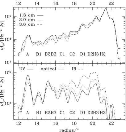
Here, we present new observations, which constitute a unique data set in terms of resolu- tion and wavelength coverage for any extragalactic jet — only M87 is similarly well-studied [84]. Using these observations at wavelengths 3.6 cm, 2.0 cm, 1.3 cm, 1.6µm, 620 nm and 300 nm, we derive spatially resolved (at 0.003) synchrotron spectra for the jet. By fitting syn- chrotron spectra according to Heavens & Meisenheimer [34], we derive the maximum particle energy everywhere in the jet and aim to thus identify regions in which particles are either predominantly accelerated or lose energy. A detailed comparison of the observed and fitted spectral shapes will test the assumption that the entire observed continuum from radio to
5For the conversion of angular to physical scales, we assume a flat cosmology with Ωm = 0.3 and H0 = h70×70 km s−1Mpc−1, leading to a scale of 2.7h−170kpc per second of arc at 3C 273’s redshift of 0.158 (see App. D).
6We define the spectral indexαsuch thatfν∝να.
ultra-violet (and possibly even X-rays) can be explained as synchrotron radiation from a single electron population.
The derived shape for the electron energy distribution will be an invaluable help in de- termining the emission process responsible for the X-rays, and we will look for correlations between the fitted synchrotron spectra and the X-ray observations. Subtle deviations from the fitted spectral shape will be a guide for future investigations into the nature of the deriva- tions, and the physical conditions giving rise to the observed emission. Only trough a detailed understanding of this jet, and its similarities with and differences to that in M87, can we hope to set the agenda for a study of other extragalactic jets.
Observations and data reduction
2.1 Observations
2.1.1 Radio data
The jet has been observed at all wavelength bands available at the NRAO’s Very Large Array (VLA), i. e., at 90 cm, 20 cm, 6 cm, 3.6 cm, 2 cm, 1.30 cm and 0.7 cm. Observations were carried out between July 1995 and November 1997, to obtain data with all array configurations (thus covering the largest range of spatial frequencies). Total integration times are of order a few times 10,000 s in each band. At 3.6 cm, the best achievable resolution (set by the maximum VLA baseline of just over 30 km) is 0.0024, with better resolution at shorter wavelengths.
However, at 0.7 cm, only few antennas were equipped with receivers at that time, and the flux density of the jet is so low that only the hot spot is detected even at a fairly low resolution of 0.0035. Observations were carried out in spectral line mode, in which the observing bandwidth of 12.5 MHz was split into 16 channels, each of which is correlated independently of all others.
The spectral line mode was chosen because an image of the jet in 3C 273 with a dynamic range exceeding 200,000:1 had been obtained at a wavelength of 6 cm and with 0.004 resolution [80]. Such a high dynamic range is necessary to simultaneously image the quasar itself, which is a strong radio source, and the faintest features of the jet. Similarly high dynamic ranges were expected to be achievable at shorter wavelengths, that is, higher resolution.
A combination of the 6 cm data with observations obtained at the United Kingdom’s Multi- Element Radio Linked Interferometer Network (MERLIN), which has significantly longer baselines than the VLA, was attempted in order to enhance the resolution and match them with the rest of the data set, to enhance the wavelength coverage. The MERLIN interferomet- ric array consists of 8 radio telescopes, of which 6 are fitted with receivers atλ6 cm. MERLIN has baselines up to 217 km, yielding a maximum resolution of 0.0004 atλ6 cm, about ten times better than the VLA at this wavelength. However, due to problems with the flux calibra- tion between these data sets, the combined image could not yet be used (see Sect. 2.2.1).
Therefore, the present analysis considers the data at 3.6 cm, 2 cm and 1.3 cm. The common resolution was fixed at 0.003, slightly inferior to the resolution of the data at 3.6 cm.
2.1.2 Optical and ultraviolet data
Optical and ultraviolet observations were made using the Planetary Camera of the second Wide Field and Planetary Camera (WFPC2) on board the Hubble Space Telescope on March
9
WF 4
WF 3
WF 2 PC 1
G
B’
X 3C 273 = Q
Figure 2.1: The field of view of the Wide Field and Planetary Camera 2 superimposed on a direct R-band image obtained at the ESO/MPG 2.2 m telescope at La Silla by H.-J. R¨oser and K. Meisenheimer.
The stars are labelled as in [87].
23rd and June 5th/6th, 1995, through the filters F300W (centered near 300 nm) and F622W (centered near 620 nm, roughly corresponding to RC in the Kron-Cousins-system).
The WFPC2 is one unit consisting of four separate cameras, the Planetary Camera (PC1) and three identical wide field cameras (WF2–4). The physical pixel size and scale of the Planetary Camera is half that of the Wide Field Cameras. Together, they map a contiguous area of the sky with the characteristic chevron shape (Fig. 2.1). The Planetary Camera has a 800×800 pixel Loral Charged Coupled Device (CCD) chip as detector. The camera has a (nominal) pixel scale of 0.0455400 at f /28.3. The resulting size of the field of view is 36.400×36.400.
The pointing and roll angle of the telescope were chosen under the following considerations.
The jet should be imaged at the centre of the Planetary Camera chip, in order to minimise any optical distortion effects. The quasar core has to be used as position reference when combining data taken by different instruments; the exact relative location of its image can be most easily determined if it is on the same chip as the jet image. An exact matching of these observations with those taken by other instruments is facilitated by having as many point sources imaged as possible, to allow the accurate determination of both shifts and rotations.
In our case, there are only four point sources in the vicinity of the jet: the quasar core and three field stars [Table 3 in 87]. The pointing and roll were therefore chosen such that each star is imaged on a separate WF chip, the quasar is near a corner of the PC and the jet is near its centre. In addition, allowance is made for small pointing offsets, which help in removing artifacts introduced by the camera pixels.
The total observing times would ideally be such that the jet features have a similar signal- to-noise ratio in both filters. The exposure time in the red wavelength band was chosen as 10 ksec which enables imaging of the jet knots at a pixel S/N of around 25, while the inter- knot regions still have aS/N of 7–10. The jet flux decreases towards shorter wavelengths. As
the CCD camera becomes less sensitive in the UV region, the exposure time to achieve the sameS/N becomes significantly larger. The total exposure time in the UV band was therefore fixed at 35.5 ks, which gives a typical pixelS/Nof 10 in most of the knots, a value of 20 only in the brightest knot, and only marginal detection of the inter-knot regions. The corresponding aperture signal-to-noise ratios at 0.003 beam size will be larger by a factor of about 10. Despite the lowerS/Ncompared to the optical data, the ultraviolet data are important in determining the shape of the synchrotron spectrum at the highest electron energies with the high spatial resolution afforded by the HST.
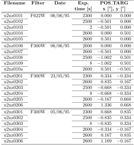
All exposures are grouped into three visits1, distinguished by the first two digits of the file number. The total exposure time was split into single integrations of around 2500 s each, the longest possible duration of roughly one half of a full HST orbit2. The U-band images are read noise limited (see Sect. A.2), therefore the longest possible integration time was chosen, resulting in 16 individual exposures at different pointings. In theR-band, the total exposure time was split into four single exposures at different pointings. These are sky background limited, but more splits would only have increased the amount of raw data having to be processed. The exposure time was therefore chosen to be one orbit for each individual exposure. An observation log is given in Tab. 2.1.
2.1.3 Near-infrared data
The near-infraredNICMOScamera 2 [“NIC2”; see 11, 101] on boardHSTwas used to image the jet through filter F160W (centered at 1.6µm), on February 6th and March 3rd/5th, 1998, as HST proposal 7848. This wavelength is critical in precisely and accurately determining the cutoff frequency along the jet. The total exposure time was 34560 s. NIC2 has 256×256 pixels of size ≈ 0.00076 on sky, making it well-suited for diffraction-limited observations at 1.6µm (Rayleigh criterion for the HST’s 2.4 m aperture, 0.0017). The field of view is just under 2000squared, significantly smaller than that of WFPC2. In fact, the detector scale along the x axis is 0.9% larger than that of the y axis, because of a tilt of the detector plane with respect to the camera focal plane. In addition, there is a global scale change with time because of expansion of the dewar assembly which moves the detector plane [Sect. 5.4 in 22]. Both effects are ignored in the reduction process and instead accounted for by appropriate placement of photometry apertures (see Section 3.1). The array consists of four quadrants which are read out separately from each other.
For these observations, the telescope was rotated such that North is approximately along the positive x direction of the detector, and correspondingly East along the positive y direc- tion.
1A “visit” is the term for “a group of exposures to be executed together”. The telescope pointing is established and guide stars are acquired at the beginning of a visit.
2HST observing time is allocated as a number of actual spacecraft orbits of duration 97 min. Depending on the telescope’s orientation and the location of the target on sky, it is observable for the full orbit or, as was the case here, for only half of the orbit due to obscuration by the Earth.
Filename Filter Date Exp. POS TARG time [s] x [00], y [00] u2nz0101 F622W 06/06/95 2300 0.000 0.000
u2nz0102 2500 −0.501 0.000
u2nz0103 2 −0.501 0.000
u2nz0104 2600 0.000 0.501
u2nz0105 2600 0.501 0.000
u2nz0106 F300W 06/06/95 2600 0.000 0.000
u2nz0107 2600 −0.501 0.000
u2nz0108 2500 −1.002 0.501
u2nz0109 8 −1.002 0.501
u2nz010a 2600 0.501 −0.501
u2nz0201 F300W 23/05/95 2300 0.334 −0.334
u2nz0202 2600 0.835 0.167
u2nz0203 2500 −0.668 −0.334
u2nz0204 8 −0.668 −0.334
u2nz0205 2600 −0.167 0.668
u2nz0206 2600 1.336 0.668
u2nz0301 F300W 05/06/95 2300 0.668 0.835
u2nz0302 2500 −0.835 0.334
u2nz0303 8 −0.835 0.334
u2nz0304 2600 −0.334 −0.167
u2nz0305 2600 0.167 0.835
u2nz0306 2600 1.169 −0.167
Table 2.1: Observation log of proposal 5980. ThePOS TARGcolumn refers to commanded offsets from the reference pointing between exposures
2.2 Data reduction and calibration
2.2.1 VLA data
Calibration and imaging
The process of calibrating the interferometric data obtained at the VLA and deriving images of the surface brightness distribution on sky was carried out by R. E. Perley (NRAO, So- corro). He supplied files containing total-intensity images as well as polarimetric information (polarised flux, degree of polarisation, polarisation angle). Details of the data reduction and a full study of the jet at radio wavelengths will be presented elsewhere [R. Perley,in prep.].
Figure 2.2 shows the three images used here.
Error sources
While the error sources for the HST images are well-known and quantified, the transformation of interferometric fringes to images introduces uncertainties which are not easily quantified [80]. An absolute flux calibration is not straightforward for radio data since the measurement
K-band 1.3 cm
U-band 2.0 cm
X-band 3.6 cm
Figure 2.2: VLA images employed in this work
of absolute radio fluxes is difficult. Therefore, most observations rely on a calibration relative to standards established by Baars et al. [3], which is probably correct to 1–2% up to 23 GHz [R. Perley, priv.comm.]. The second problem for radio data is related to the fact that the brightness distribution on the sky cannot be inferred uniquely from the fringe patterns it produces through an interferometer because the deconvolution involved in the inverse process is not unique. Thus, although the noise on the actually detected signal is well-known, there is no good estimate on how this translates to noise in the image plane. In addition, there may be artifacts present in the image, i. e., errors in the sense that the inferred brightness distribution does not correspond to the true brightness distribution. The usual way to quote the quality of a radio map is the “dynamic range”, defined as the ratio of the peak surface brightness to the RMS noise of a blank region of sky. This RMS noise is the single quantifiable noise estimate for radio maps and a lower limit to the true precision. Table 2.2 quotes the dynamic ranges for the images used here. From the table, it is clear that the dynamic ranges which were actually achieved fell considerably short of the expectations.
Combination with MERLIN data
In order to enhance the resolution of the VLA data set atλ6 cm, a combination was attempted with MERLIN data. The VLA interferometric data set comprising the calibrated data was
VLA band λ Peak flux RMS noise Dynamic range
cm mJy mJy
C∗ 6 35.9 6.0×10⁻⁴ 80,000
X 3.6 33.0 4.5×10⁻⁴ 75,000
U 2.0 28.3 2.6×10⁻⁴ 110,000
K 1.3 23.4 4.0×10⁻⁴ 59,000
Q∗ 0.7 20.9 2.5×10⁻³ 9,000
∗image not used for spectra
Table 2.2: Dynamic ranges for the VLA images
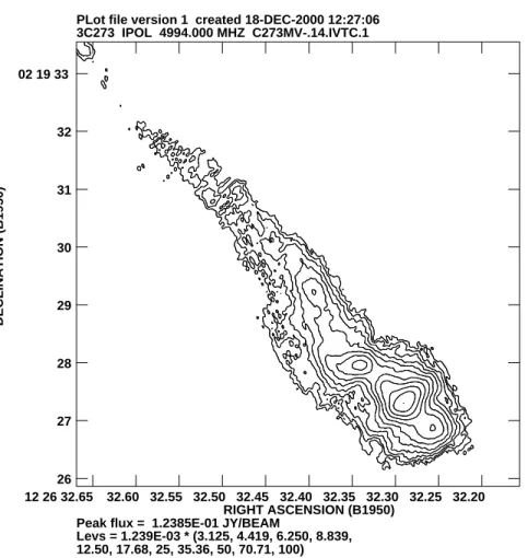
3C273 IPOL 4994.000 MHZ C273MV-.14.IVTC.1 PLot file version 1 created 18-DEC-2000 12:27:06
Peak flux = 1.2385E-01 JY/BEAM
Levs = 1.239E-03 * (3.125, 4.419, 6.250, 8.839, 12.50, 17.68, 25, 35.36, 50, 70.71, 100)
DECLINATION (B1950)
RIGHT ASCENSION (B1950)
12 26 32.65 32.60 32.55 32.50 32.45 32.40 32.35 32.30 32.25 32.20 02 19 33
32
31
30
29
28
27
26
Figure 2.3: Map obtained from a combination of MERLIN and VLA data atλ6 cm.
merged with a coeval MERLIN data set provided by Simon Garrington and Tom Muxlow (Jodrell Bank Observatory). The joint data set was then imaged using a maximum entropy deconvolution method to obtain a map of the jet comprising the information on all the angular scales sampled by either telescope array.
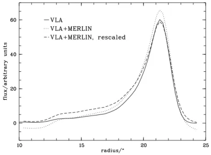
The combined map is shown in Fig. 2.3. Although the map looks morphologically plausible, a comparison of the derived jet profile with the original VLA map shows a discrepancy between the two (Fig. 2.4). The total flux of the combined map is about 20% larger than that
Figure 2.4: Comparison of VLA and VLA+MERLIN data sets at 1.003 resolution. The jet profile derived from the combined data set is discrepant from that obtained from the VLA observations alone.
detected by the VLA alone, and the background flux level is not zero, but slightly negative.
An attempt of correcting both background offset and flux normalisation error was made by adding a constant to the combined image to make the average background level zero, and then scaling the jet image to match the total flux contained in both. As Fig. 2.4 shows, after this normalisation attempt, the jet profile at 1.003 resolution is still discrepant between both data sets.
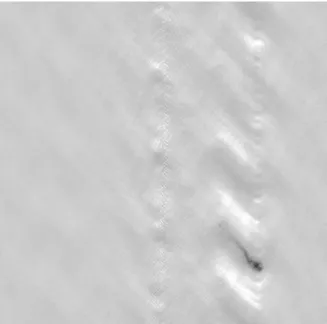
The reasons for the discrepancy are not known in detail at present. They are most likely related to the strong north-south sidelobes of the MERLIN array. A two-element interfer- ometer is sensitive only to structures perpendicular to its baseline. Unlike the VLA with its three-armed configuration, MERLIN has predominantly north-south baselines. Therefore, it best samples structures oriented in an east-west direction for sources observed on the merid- ian. For sources at large declinations, the Earth’s rotation provides for a rotation of the baselines on the sky, so that all parts of the (u, v) plane (the “k-space” for celestial coordi- nates) are observed and structures at all position angles on sky can be detected (aperture synthesis technique). However, since 3C 273 is located near the celestial equator, the geometry of the MERLIN array leaves structures in extending in a north-south direction ill-constrained.
Periodic positive and negative images of the jet appear to the north and south of the true image (Fig. 2.5).
Detailed investigations will be required to remedy the flux discrepancy between the VLA- only and the joint VLA-MERLIN data set. MERLIN data are also available at λ18 cm, a combination with VLA data will only be attempted once the λ6 cm data are understood.
2.2.2 WFPC2 data reduction steps
The WFPC2 data reduction for this project has already been described in detail previously [41], we therefore give an outline here and present details in App. A.
Images taken with CCD cameras have to undergo certain data reduction and calibration
Figure 2.5: The MERLIN image atλ18cm shows the positive and negative images of the jet caused by the array’s sidelobes.
steps to remove instrumental effects like variable detector response etc. After execution of a science program, the STScI provides pipeline-calibrated science frames along with the raw exposures. As some of the calibration information may have been updated since the pipeline calibration, the images have been recalibrated. The recalibration was done under IRAF, using the taskcalwp2, part of theSTSDAS(Space Telescope Science Data Analysis System) package provided by the STScI. This task calls subroutines applying the individual calibration steps, using information saved with the data frames to determine the appropriate calibration files.
The best calibration files were obtained from the STScI archive.
The value for background noise measured on the calibrated images agrees with the values expected from photon statistics, as calculated from the predicted sky background level, read noise and dark current (Sect. A.2). One of the PC chip’s charge traps [105, 107] lies inside the jet image, in column 339. This has no observable effect on the faint UV image, but the effect had to be corrected on the well-exposed red-band images. This was done by replacing the affected portion of each image by the corresponding pixels from an offset image, as a correction according to Whitmore & Wiggs [107] unduly increased the noise gin the corrected part of the image (Sect. A.3.1).
The images were initially registered using the commanded offsets to the nearest pixels.
This alignment is sufficient for the rejection of cosmic rays as these only affect a small number of adjacent pixels. Cosmic rays were removed using a standard κ-σ algorithm, rejecting all pixel values deviating more than 4σ from the local (low-biased) median in a first pass, and neighbouring pixels with more than 2.5σ deviation in a second pass (details in Sect. A.3.3).
The number of pixels treated this way agrees with the expected cosmic ray hit rate for the images.
A model of the sky background and “horizontal smear” (increased pixel values in rows containing saturated pixels from the quasar’s core [Chap. 4 of 8]) was fitted in the part of the image containing the jet using second-order polynomials along rows (Sect. A.3.4). The
Filter PHOTFLAM λp PHOTFNU F300W 6.137×10⁻¹⁷ 2981.9 17.72 F622W 2.789×10⁻¹⁸ 6187.5 3.531
Table 2.3: Photometric conversion factors. PHOTFLAMis in erg s−1cm−2˚A−1,λpin ˚Angstrøm,PHOTFNU is inµJy.
coefficients of the polynomials were then smoothed in the perpendicular direction.
The photometric calibration of the exposures was done using throughput information provided in [8, Section 21.1.2]. A synthetic photometry approach is employed: The combined response of telescope, filter and detector is used to calculate the physical flux producing a count rate of 1 count per second in each filter. A constant flux per unit wavelength is assumed. The proportionality factor between count rate and spectral flux density is given in units of erg s−1 cm−2 ˚A−1 and referred to asPHOTFLAM. For the later comparison with radio astronomical measurements, which are commonly calibrated in Jansky (Jy, 1 Jy = 10−26 W m−2 Hz−1), the count rate is converted to Jy. The corresponding conversion factor is called PHOTFNU. The spectral flux per unit wavelength fλ is converted to a flux per unit frequency fν by noting that
fλdλ=−fνdν (2.1)
(The−sign arises because dν increases in the opposite sense to dλ.) From here, fν =−dλ
dνfλ = λ2
c fλ (2.2)
This is, strictly speaking, only valid at a single value pair forλandν. In order to obtain the correct spectral flux density conversion, the shape of the input spectrum would have to be convolved with the throughput curves over the filter passband. As the input flux spectrum is not known a priori, but is rather what we are trying to measure, this would have to be done in an iterative fashion: calculate a flux density assuming a spectrum constant in each passband, fit a spectral shape to measurements across the whole spectrum, then refine the flux density conversion using the spectral shape in each passband.
It will be sufficiently accurate here to convertPHOTFLAMtoPHOTFNUusing thepivot wave- length λp of each filter used. The pivot wavelength is a characteristic of the filter. It is defined such that Eqn. 2.2 is true withλ=λp, andfν and fλ being obtained by integrating a spectrum with constant flux per unit frequency or wavelength, respectively, over the bandpass transmission curve (see Sec. 18.2.2 of [105] and [12]). The conversion between the different units ofPHOTFLAM and PHOTFNU introduces a numerical factor of 1033 which arises from the definition of 1 Jansky and the conversion from erg to W (1W = 107 erg).
The best values for the count-to-flux calibration, filter pivot wavelength and resulting flux in Jansky for 1 count per second are given in Tab. 2.3.
The throughput information is accurate to 2% if the most recent values are employed.
The flux calibration is done by dividing the data frames by the exposure time (to give a count rate) and multiplying by the respective value ofPHOTFNU.
With this calibration, the background uncertainty parameters (Sect. A.3.4) scale to the following values: the background scatter in the summedU and R-band images are 0.35 nJy and 0.14 nJy, respectively. The residual background levels are 0.07 nJy and 0.01 nJy per pixel, respectively.
1" N
E
H2 extension
Southern
H3 D2 Inner extension
C2
D1 C1
B2 B3 A B1
Star
Outer extension
= galaxy S
In2 In1
Figure 2.6: The jet in red light (620 nm) after background subtraction. Logarithmic grey-levels run from 0 to 0.04µJy/pixel, 0.0008 effective beam size, 0.00045 pixel size. The quasar core lies 1000 to the northeast from A. The labelling of the jet features as introduced by Leli`evre et al. [52] and extended by R¨oser &
Meisenheimer [87], together with the hot spot nomenclature from Flatters & Conway [27] is also shown.
Note that the labelling used by Bahcall et al. [4] is slightly different.
2.2.3 Maps of the optical brightness
The calibrated images are presented in Figs. 2.6 and 2.7. The morphology of the jet is identical in both images and appears rather similar to the morphology in high-resolution radio maps [4, 17]. The exception to this is the radio hot spot, being the dominant part in the radio but fairly faint at high frequencies (a detailed comparison follows in Sect. 3.2). Our images show structural details of the optical jet which were not discernible on earlier, shallower and undersampled HST WF images of 0.001 pixel size [4]. Based on our new maps, the term
“knots” seems inappropriate for the brightness enhancements inside the jet, as these regions are resolved into filaments. The higher resolution necessitates a new nomenclature for the jet features (Fig. 2.6). For consistency with earlier work [27, 52, 87], our nomenclature is partly at variance with that introduced by Bahcall et al. [4].
The jet is extremely well collimated – region A has an extent (width at half the maximum intensity) of no more than 0.008 perpendicular to the average jet position angle of ∼ 222◦ (opening angle<∼5◦). Even H3 is only 100wide along the longest axis (opening angle ≈2.5◦).
The optical jet appears to narrow towards the hot spot, in the transition from H3 to H2.
Region A is now seen to extend further towards the core than previously known. It may be noteworthy that Leli`evre et al. [52] reported the detection of an extension of knot A towards
1"
E N
Figure 2.7: The jet in UV light (300 nm) after background subtraction. Logarithmic grey-levels run from 0 to 0.014µJy/pixel, 0.0006 effective beam size, 0.00045 pixel size.
Figure 2.8: After modelling the background near the quasar and smoothing the 620 nm image to 0.0025, the faint inner 1000of the optical jet can be made out.
the quasar, whose existence at the reported flux level was not, however, confirmed by later work.
When considering a smoothed version of the summed WFPC2 image, a faint continuation of the optical jet can be made out (Fig. 2.8). Bahcall et al. [4] also reported a tentative detection of this inner jet. In order to establish a reliable detection, we have obtained deep optical images of the jet with the FORS1 instrument at the ESO Very Large Telescope (VLT).
For these data, the accurate modelling and subtraction of the background due to the quasar PSF (with a seeing-limited FWHM of around 0.007) turned out more difficult than anticipated and results will be reported elsewhere.
The criss-cross pattern visible in regions C1 and C2, and less clearly in B1-2 and D1, is reminiscent of a helical structure, possibly double [4], but could also be explained by oblique double shocks [31, e. g.].
The jet has three “extensions” (Fig. 2.6), none of which has been detected at radio wave- lengths. The morphology of theouter extension supports the classification as a galaxy based on its colours made by R¨oser & Meisenheimer [87]. The nature of the other two extensions, however, remains unknown even with these deeper, higher resolution images. Thenorthern inner extension was already resolved into two knots (In1, In2) on aFaint Object Camera image [102]. The two knots are extended sources and clearly connected to each other. The southern extension is featureless and an extended source.
Comparing the direct images, we can immediately estimate that the jet’s colour slowly turns redder outwards from region A. The similarity of the jet images in both filters shows that there are no abrupt colour changes within the jet. A comparison of these images with those at other wavelengths is deferred to Sect. 3.2. A quantitative assessment of the jet’s colour will be done through resolution-matched spectral index maps in Sect. 3.5.2.
2.2.4 NICMOS data
Like optical CCDs, today’s near-infrared detectors make use of the photoelectric effect for the detection of light. The semiconductor material used in the NICMOS3 detector employed in the NICMOS camera is mercury cadmium telluride (HgCdTe), which has a band gap suitable for the detection of near-infrared photons. Unlike a conventional CCD, in which the accumulated charge is transferred out of the detector array for read-out, the NICMOS3 detector can be read out non-destructively. Apart from this, an IR detector has a bias level, dark current and readout noise just like an optical CCD, with analogous reduction steps. To keep the detector from detecting itself, it is cooled to liquid-helium temperatures.
Because of thermal emission from the sky (for the HST this is the solar-system dust emit- ting the zodiacal light) and the telescope itself, the background levels for IR observations are much higher than those for optical wavelengths. Ground-based telescopes suffer from still higher background levels than the HST: Firstly because the atmosphere is a much warmer emitter than zodiacal light, and secondly because of telluric absorption and emission (“air- glow”, mainly from from OH− and O2). The ground-based near-IR filter bands J, H, K at 1.2, 1.6 and 2.2 µm are designed to lie between the telluric features, but cannot avoid some of the numerous airglow lines. The present observations were carried out at a wavelength of λ ≈ 1.6µm, at which the total background due to both sky and telescope is at a mini- mum for the HST [11]. They therefore constitute the deepest near-infrared exposure of any extragalactic jet so far.
Description of NICMOS data
Because of the possibility of non-destructive readout,reset andread out are two separate and independent operations for the NICMOS detector. While the reset clears all accumulated charge from the detector, it leaves the array at an uncertain bias level. The array is therefore read out immediately after the reset to obtain the so-calledzeroth read, which is subtracted from subsequent reads to obtain the true signal. This means that the readout noise enters into each NIR image at least twice.
The total exposure time was split over three HST visits with 10 exposures each. Because
the field of view is not much larger than required to image the quasar and jet simultaneously, there is one short image of the QSO at the beginning of each visit. Each individual visit comprises five pairs of jet exposures, each pair placing the jet on a different part of the detector. One of the exposures per pair has exposure time 1024 s, the other 1280 s. There are additional interspersed sky exposures of 256 s.
Following a recommendation from STScI, the present images were taken in the so-called MULTIACCUM mode, with readouts 0, 0.3, 0.6 s after the reset, and then every 256 s. Using this exposure mode, it is in principle possible to obtain the count rate for each pixel by fitting the relation between observed counts and observing time. Cosmic ray rejection should also be facilitated, because a cosmic ray hit can be identified as discontinuity in the observed relation.
However, with the exposure times and time step chosen, each data set consists of only 4 or 5 independent data points (there is hardly any signal in the first, very short readouts), so that full advantage of the MULTIACCUM capability was not taken.
A pipeline softwareCALNICA, provided by STScI, exists to carry out the reduction of all NICMOS data. This pipeline performs the following steps for the present data:
• correction of the zeroth read for detectable signal (above 5σ) incurred in the 0.2 s elaps- ing between reset and read operation for each pixel
• subtraction of the zeroth read from each subsequent read
• subtraction of an appropriate dark image from each read
• correction of detector non-linearity according to an empirical cubic relation
• correction of “bars” — small, noiseless bias changes in a pair of rows (one elevated, one lowered), replicated in all four quadrants
• flat-field correction
• linear fit to relation of counts vs. observing time, rejection of cosmic rays as outliers from the relation
A number of more or less subtle error sources which are not accounted for by this procedure meant the pipeline reduction was inappropriate for the present data. This necessitated the use of a tailor-made reduction procedure, whose outline follows the pipeline method. After a consideration of these error sources, we will turn to a description of the steps finally taken for the reduction of the NIC2 data.
Error sources for HST NICMOS
The main error source identified for our data is a spatial and temporal variation of the bias level. The true bias for each readout has three components [74]:
1. “normal” bias introduced at reset (different for each reset),
2. “shading”, a readout bias which is variable with the time since last readout and the temperature,
3. and “pedestal”, a random change of the overall bias level per quadrant.
Figure 2.9: Example of the pedestal effect in NICMOS images. The background level differs clearly from quadrant to quadrant, and the flat-field imprint is visible.
The first component is taken care of by the usual zeroth read correction. The “shading”
means that in fact the readout bias varies over each quadrant, leading to a bias structure in each readout, while the overall level depends on the time since the last readout. In addition to this temporal bias variation, there is a temperature dependence, which may introduce an additional variation of the bias level from readout to readout. The variation of the shading from one read to the next is probably the cause of the third effect, the pedestal, which appears in the data as offset between the quadrants of one image (see Fig. 2.9).
The joint effect of the bias variations is that the pipeline calibration does not remove the true bias. Since the bias is additive and not subject to the sensitivity variations which are removed by flat-fielding, the pipeline-calibrated image contains an imprint of the flat- field structure: assume a total raw signal I(x, y) was detected on the pixel with coordinates (x, y). This signal consists of the signal from the sky,S(x, y), modulated by the sensitivity pattern f(x, y), and the bias B(x, y), which does not modulate with the flat-field. A wrong bias subtraction leaves a residual bias ∆B(x, y). After correction with the flat-field pattern f−1(x, y), which is the inverse of the sensitivity and assumed to be known, the calibrated signalC(x, y) is
C(x, y) = f−1(x, y) (f(x, y)S(x, y) + ∆B(x, y))
= S(x, y) +f−1(x, y)∆B(x, y),
so that the resulting image contains an imprint of the flat-field pattern, while the sky signal has been adequately corrected. As the sensitivity variations are rather large for NICMOS (factor of 5 at 0.8µm, decreasing to near unity at 5µm; cf.Fig. 2.10), the residual signal contained in the flat-field imprint is considerable. In addition, “pedestal” offsets between the detector quadrants remain. The offsets could in principle be removed a posteriori, by estimating a constant pedestal level per quadrant and equalising the quadrants, e. g. It is desirable, however, to correct the bias to the best available knowledge before flat-fielding,
Figure 2.10: NIC2 flat-field frame. Oversensitive pixels appear dark, undersensitive pixels bright. Bright specks are “grot”, pixels with drastically reduced sensitivity.
thus minimising the flat-field imprint, and before the estimation of count rates from the slope of the counts-vs.-time relation. One readout with a wrong bias level in the four or five reads per image may well lead to a systematically wrong slope, thus necessitating a multiplicative correction rather than an additive one.
A number of correction algorithms for this effect are publicly available. Their essence is to assume that the true signal should accumulate linearly with time, or that the true background is flat, and subtract a constant times the flat-field image from the calibrated data to optimise the result according to the chosen criterion. All of the available algorithms failed to remove both the offsets between quadrants and the flat-field imprint.
As the variation of bias level with temperature is systematic and reproducible, the NIC- MOS group have provided a tool to generate temperature-dependent dark files, with a bias appropriate for the readout temperature [75]. Using a temperature-dependent dark accurate to 0.05 K should significantly alleviate the bias problems. However, even using separate darks for each readout to 0.01 K did not improve the quality of the reduced images.
In addition to the bias variations, column number 128 is known to be a “bad column”
with a bad bias level and elevated noise. A number of small patches of few pixels with reduced sensitivity is known as “grot”. Finally, the sensitivity of the NICMOS pixels is wavelength-dependent, in the sense that oversensitive pixels are less sensitive toward longer wavelengths, while undersensitive pixels have sensitivity increasing with wavelength. This colour dependence of the flat-field means that the calibration flat-field taken with an internal lamp may not be appropriate for the sky or object. The effect of the colour dependence for the sky background is most severe at wavelengths above 1.8µm [74]. Its effect is difficult to disentangle from the flat-field imprint left by the bias problems.
To remove these effects, in particular to remove the bias offsets between the quadrants, a completely different reduction procedure was implemented.
Reduction steps taken
In order to remove the calibration errors, some assumptions had to be made about the data and calibration errors, to constrain the number of free parameters. In particular, we assumed that
• the internal lamp flat-field is correct,
• the true sky is flat,
• the dependence of the bias level on the time since the last readout is identical for all images,
• and any further bias variation between readouts is constant within each quadrant of every readout.
We assume that the flat-field is correct because of the lack of information of what the true flat-field otherwise would be. The sky exposures which have been taken are short compared to the science exposures and hence noisy, and of course suffer from the same bias uncertainties as the object exposures. They provide therefore no further information. The assumptions about the bias have to be made to allow any correction at all.
The reduction algorithm’s essence is the joint estimation of all background signals (dark current, sky signal, bias) after filtering the object (and cosmic ray) signal out of the frames.
This is possible because the exposures were taken at 15 different pointings. Hence the object moves around the detector, while the background remains unchanging. Each readout has a different bias. All readouts are therefore grouped into image cubes of readouts with identical exposure time. For each detector pixel, the background signal is estimated as the lower quartile value of the distribution of pixel values across the readouts (30 with exposure times up to 1024 s, 15 with exposure time 1280 s). The lower quartile value is chosen rather than the median to be sure to exclude object and cosmic-ray signal (see Fig. 2.11). The background value is subtracted from the pixel in each readout.
This step has removed the dark current, sky background and all bias components which vary across the detector, but not from readout to readout. To remove the quadrant-to- quadrant variations, the residual background in eachquadrant of every readout is estimated and subtracted separately. The background estimation is done using the routineMMM within theIDLgraphics package. This initially rejects positive outliers (signal, cosmic rays) from the pixel value distribution byκ-σ-clipping and uses the mean as sky estimator, or 3×median - 2×mean if the mean is larger than the median.
As a drawback of this approach, the knowledge of the sky and dark signal cannot be used to estimate the noise associated with these components any more. Instead, the noise will be estimated in the photometry by considering the scatter of calibrated pixel values. After the treatment, the images contain only the object counts and cosmic rays. The quadrants are reassembled into images, and the count rate is estimated and cosmic rays are rejected using the programfullfitbam[59], which is derived from that used by the pipeline software CALNICA.
Since the cosmic ray rejection byfullfitbam is not perfect, a cosmic-ray rejection using COSMIC/MEDIAN (as for the optical data) is performed. For this step, all known bad pixels (including column 128 and the “grot” mentioned above) and negative outliers are flagged so that they, too, are replaced by the cosmic-ray rejection routine. The resulting images are not