SFB 649 Discussion Paper 2011-045
Bayesian Networks and Sex-related Homicides
Stephan Stahlschmidt*
Helmut Tausendteufel**
Wolfgang K. Härdle*
* Humboldt-Universität zu Berlin, Germany
** Berlin School of Economics and Law, Germany
This research was supported by the Deutsche
Forschungsgemeinschaft through the SFB 649 "Economic Risk".
http://sfb649.wiwi.hu-berlin.de ISSN 1860-5664
SFB 649, Humboldt-Universität zu Berlin
S FB
6 4 9
E C O N O M I C
R I S K
B E R L I N
Bayesian Networks and Sex–related Homicides ∗
Stephan Stahlschmidt
Ladislaus von Bortkiewicz Chair of Statistics Humboldt–Universit¨at zu Berlin
and
Centre for Social Investment Heidelberg University
Helmut Tausendteufel
Department of Police and Security Management Berlin School of Economics and Law
Wolfgang K. H¨ ardle
Ladislaus von Bortkiewicz Chair of Statistics Humboldt–Universit¨at zu Berlin
Abstract
We present a statistical investigation on the domain of sex–related homicides. As general sociological and psychological theory on this specific type of crime is incom- plete or even lacking, a data–driven approach is implemented. In detail, graphical modelling is applied to learn the dependency structure and several structure learn- ing algorithms are combined to yield a skeleton corresponding to distinct Bayesian Networks. This graph is subsequently analysed and presents a distinction between an offender and a situation driven crime.
Keywords: Bayesian Networks, structure learning, offender profiling JEL classification: C49, C81, K42
AMS clasification: 62-09, 62P25
∗The financial support from the Deutsche Forschungsgemeinschaft via SFB 649 ” ¨Okonomisches Risiko”, Humboldt-Universit¨at zu Berlin, and the Bundeskriminalamt is gratefully acknowledged.
1 Introduction
Criminal profiling can be defined as the process of identifiying a suspect’s be- havioural characteristics and principal personality from a crime scene. Police pro- filers firstly analyse the crime scene carefully and deduce the exact course of events.
Based on this groundwork they try to discover why theses events occurred and fi- nally what type of person could have committed these acts. The method thereby relies on certain assumptions, most notably the belief that the criminal’s personality can be retrieved from the crime scene.
Gaining a psychological and social profile of the suspect has several advantages for the police. Known characteristics of the offender can narrow the number of po- tential suspects by excluding those not showing the specific traits. This hopefully leads to a faster arrest of the criminal, but also reduces costs for the police and so- ciety. Furthermore the knowledge may lead to certain investigative strategies and, as people show different reaction to police interrogation approaches, prove useful during questioning of other suspects.
The wide and successful application of offender profiling has been enhanced by scientific background knowledge. To this end statistical techniques, like multidi- mensional scaling, cluster analysis or logistic regression have been applied to data of resolved crimes. This data has been generated by collecting evidence on the crime scene and learning the characteristics of the convicted offender by an interview or the criminal’s record. An overview of the applied techniques is given by Beauregard (2007). However most studies concentrate on a rather broad typology or predict only single variables, e.g. Davies (1997) and Salfati and Canter (1999). Therefore Aitken et al. (1996) propose the application of Bayesian Networks (abbr. BN) based on expert knowledge and Baumgartner et al. (2008) learn the structure of a BN for criminal profiling from data.
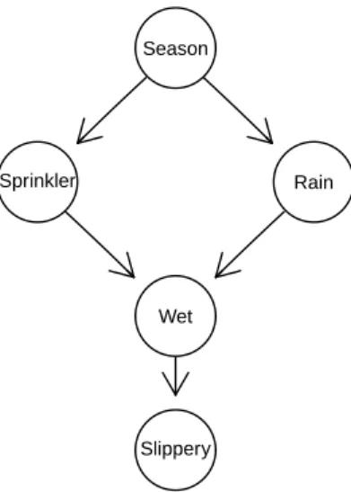
Although the use of BNs on data of crimes is a new and promising application, the technique itself has already been applied to several fields such as crop failure (Wright, 1921), medical diagonis (Heckerman, 1990) or biological networks (Fried- man et al., 2000) among others. This broad scope of BNs may be explained by its unique characteristics. A BN consists of a directed acyclic graph (DAG) which mirrors a factorisation of a probability distribution over several variables by includ- ing a directed edge between two dependent variables. Conditional independence among certain variables leads to a sparse graph, in which the nodes, represent- ing variables, can be endowed with conditional probabilities. This combination of (in-)dependence statements and conditional probabilities describes the possibly causal relations among all factors of a specific domain and facilitates thereby sta- tistical inference (Jensen, 1996). Figure 1 displays the classical sprinkler example by Pearl (2000) for illustration.
BNs offer several advantages for criminal profiling, as they describe the structure of a pre–specified domain. Hence the building of a BN mainly by data may be used for learning the structure of an unknown domain, e.g. certain types of homicides.
Furthermore BNs may also be employed for prediction. Profilers could for example obtain a prediction of the offender’s age and thereby reduce the number of suspects substantially by entering evidence found on the crime scene into an appropriate BN. Pure prediction methods as for example BART (Chipman et al., 1998) cater
Season
Sprinkler Rain
Wet
Slippery
Figure 1: BN describing the structure between five variables.
to minimise the error rate for the prediction of a single variable by adjusting model parameters and do not restrict their analysis to solely causal connections. Further- more, crime scenes often lack certain information or do not only render one course of events plausible, but several competing ones. By its very nature a BN can be exploited to order competing hypothesis according to their probability given the facts and allow for inclusion of soft evidence. These reasons make this statistical technique appealing to profilers and the purpose of this paper is to present a case study on sex–related homicides in Germany.
The restriction to sex–related homicides, resulting from requests by the German federal police, has several implications, which distinguishes our work from previous research. First, sex–related homicides occur infrequently and second the assump- tion of homology between the offender’s characteristics and the crime scene actions lacks further verification (Alison et al., 2002). Therefore, experts may name several important factors which are to be included in any systematical approach to the domain, but refrain from giving a precise ordering of these factors or detailing the exact relationships between these factors. Hence building a BN solely from expert knowledge is unfeasible and we therefore rely on a data–driven approach to learn the BN’s edges, also known as structure learning. However, data on sex–related homicides is scarce and not collected routinely like for example data on car acci- dents. We therefore accumulated a sample of sex–related homicides which occurred in Germany between 1991 and 2006. This study leads to one of the biggest and most detailed databases on this specific type of crime and we sequentially base our computation of a graphical model on this data. The data consists of 252 cases, in which the offender was found guilty by a German court, and although this repre- sents a large increase in sample size concerning former studies, it is still short of a sufficient number of cases required by well–known structural learning algorithms as specified in Zuk et al. (2006) or Baumgartner et al. (2008). The number of poten- tial edges in a BN grows exponentially in the number of variables (Robinson, 1977) and although we have more observations than variables, we have considerably fewer observations than potential edges. This situation leads to the realm of “p >> n”
and poses several challenges for structural learning which we address by combining several algorithms to find edges persisting throughout the resulting graphs.
In general, a notional scale with two oppositional prototypes of sex–related homi- cides and several increments in between can be deduced from the graphical model.
On one hand several criminals show a high level of preparation and forensic aware- ness. They apply sophisticated measures to control the victim and are more likely to exhibit a sadistic or serial background. Furthermore, more often they attack victims which are unknown to them and which they contact in unfamiliar surround- ings. These crimes carry a rather long enquiry period. On the other hand, several criminals do not show high levels of preparation or forensic awareness. Instead al- cohol often constitutes a vital part of the crime and the offenders are more likely to apply blunt force instead of more elaborated measures to control their victim. They are often known to the victim and act in familiar surroundings. Several crimes do not belong strictly to either one of these prototypes, but only exhibit some of the specified features or even show features of both prototypes. However, in any case, offenders have to interact with factors, which they cannot affect, like the victim’s resistance or the characteristics of the contact location. These and other variables mirror the applied Criminal Event Perspective, which states that the actions at the crime scene are determined simultaneously by the offender, the victim and the underlying situation.
In section 2 we report on the data collecting process. Section 3 discusses the applied technique of BNs and section 4 states the results. Finally, section 5 concludes with a discussion of these results.
2 Data collection
The lack of data on sex–related homicides may be explained by the extremely te- dious, but necessary effort needed to collect the data and secondly by the restricted access to relevant information. Although court proceedings may be open to the public, the required time to attend several lawsuits would render this approach cumbersome. Furthermore information irrelevant to the judical conviction but es- sential from sociological or psychological perspectives may not be mentioned in detail. Hence, data collection relies on the assistance from authorities with access to adequate information.
The data presented in this paper is based upon support by the German police, which drew a sample of sex–related homicides from their internal documentation and provided access to the corresponding prosecutor’s files. These files count be- tween 1,500 and 10,000 pages, of which the crime scene report, the autopsy report, the psychiatric examination of the offender and the sentence contain almost all the essential information. Among them are, for example, the victim’s injuries, the of- fender’s age or information on the contact location. Although the documents cover all the important aspects of the crime and the offender’s characteristics, this indirect access to information on the crime results in some distortion. Obviously police offi- cers arrive at the crime scene only after the crime has been committed and therefore may only collect traces of the crime without observing it directly. Furthermore the police and judicial system act on their own principles, which constitutes a further influence on the available information. And most importantly, only traces found on the crime scene are to be considered as genuine. These are seldom sufficient and tes- timonies by witnesses and the offender have to be taken into account to reconstruct the details of the crime. But as this study is concerned with homicides, especially statements by the offender can only be checked against the traces at the crime scene and may leave room for speculation and undiscovered misinformation.
CRIME
Offender Victim Underlying Situation
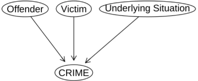
Figure 2: Schematic overview on factors influencing a crime
Transferring information from prosecutor’s files into nominal variables requires com- parable information throughout all cases. Therefore the prosecutor’s files have to be scanned to determine which content would be available for an empirical analysis.
Comparative text analysis (Strauss and Corbin, 1990) is a popular technique to se- lect the information satisfying this requirement and the variables presented in this study result from a comparative text analysis of 30 cases. However, not all avail- able information is of use and the amount of information transferred into variables is restricted to a consistent set of important factors in the domain of sex–related homi- cides. The resulting variable selection is guided by sociological and psychological theory extended by the police’s hands–on experience. This theoretic background states that predominantly soft factors, such as the offender’s disposition to com- mit a crime influence the actions at the crime scene (Mokros and Alison, 2002).
These factors cannot be measured directly, but due to their complexity may only be expressed via proxy variables. Furthermore the occurrence of several offenders, victims and/or crime scenes in a single crime poses a challenge for the storage and analysis of the corresponding data. The same holds for serial crimes, in which every single crime enters the data separately, though marked by a dummy variable.
The information analysed in this study and transferred into variables focuses on four main elements: The offender, the victim, the underlying situation and the actual offence. A schematic overview is presented in Figure 2. The offender is described by his social, psychological and economic characteristics. Furthermore information regarding his medium–term and short–term disposition to commit a crime including his criminal record and any preparation to commit the crime are collected. Infor- mation on the victim is not widely available, however indicators on her social and economic status, as well on her prior relationship status with the offender is present throughout all cases. The underlying situation with its geographical and temporal information provides the general setting of the crime. The actual offence can be split up into several categories. First, any pre–attack events regarding the offender or shared activities between the offender and the victim before the attack are taken into account. Afterwards the actual crime begins with the offender’s attack on the victim, which differs, for example, in the time needed, the victim’s resistance or the level of applied violence. Resulting injuries including the fatal ones are recorded and sexual activities imposed on the victim are observed. Finally the offender’s forensic awareness is measured and broadly divided into activities to hide his iden- tity and activities to hide the crime. Further details on the variables are available in Tausendteufel et al. (2011).
The quality and quantity of the available information is highlighted by missing values and inter–rater reliability (Fleiss, 1971). Crimes resulting in limited traces entail a higher than average percentage of missing values. The same holds if the criminal refuses to testify, as several factors cannot be deduced from traces alone.
Furthermore a high rate of missing values is accompanied by relatively low levels of inter–rater reliability. Raters seem to handle vague information differently. In general the data includes 6% missing values and Fleiss’ meassure of inter–rater re- liability between four raters amounts to κ= 0.53 with a percental match of 73%.
The actual collection of the data was carried out by reading all important doc- uments of a particular crime and entering relevant information in a standardised form. This summary with all the essential information is thereafter deployed to assign all predefined variables. On average a rater completes two of the 252 cases on a typical working day. All together it took nearly a year to provide the data for the subsequent analysis.
3 Bayesian Networks and Structure Learning
A graphG = (V, E) is defined by a set of nodesV={V1, . . . , Vp}and a set of edges E ⊆ V×V, which connect the nodes (Lauritzen, 1996). BNs form a particular subclass of graphical models and contain solely directed edges. Their set of edges E includes the entry (Vi, Vj), but not the entry (Vj, Vi) to denote a directed edge from nodeVi to nodeVj. Undirected edges are expressed as the entries (Vi, Vj) and (Vj, Vi) inE. In a directed edge (Vi, Vj) the nodeVi is known as the parent of node Vj, and recursively the nodeVj is said to be the child of Vi. The set of parents and children of a nodeVi describe its adjacency. Extending the adjacency by all further parents of Vi’s children, the Markov blanket of Vi is specified. For example in Fig- ure 1, the adjacency of node “Rain” consists of the parent node “Season” and the child “Wet”, whereas the Markov blanket of the same node also includes the node
“Sprinkler”, as it constitutes a further parent node to the joint child “Wet”. The descendants de(Vi) of any node Vi are defined by its children and any subsequent children. In order to distinguish clearly between descendants and non–descendants, we require the graph to omit circles. Consequentially the structure of a BN is known as a DAG (directed acyclic graph). A skeleton is a DAG without the arrow heads, such that all directed edges are converted into undirected edges. It includes several paths, describing a chain of nodes consecutively connected by edges. A chain of directed edges pointing all in the same direction is known as a directed path. If any two nodes point, via directed edges, at the same node without being adjacent, a collider arises. Figure 1 includes a single collider, namely the node “Wet”.
A path π in a DAG G = (V, E) is said to be blocked by a set S ⊆ V if node Vw ∈S on the path π is not a collider or some other colliderVv ∈/ S on the path π exits andVw ∈/de(Vv). Two disjoint subsetsAandB ofV ared–separated byS, if all paths betweenA and B are blocked by S (Pearl, 2000). In Figure 1, the nodes Seasonand Slipperyared–separate by the set{Sprinkler, Rain}or the single node Wet. However, the nodeRain alone does notd–separate the nodesSeasonandSlip- peryas the directed pathSeason→Sprinkler→Wet→Slipperyis not blocked by it.
The probability distribution function of a random vector X = (X1. . . Xp)> ∈ Rp
with an arbitrary ordering of the variables may be factorised as P(X) =
p
Y
i=1
P(Xi|X1, . . . , Xi−1). (1) Assuming that the conditional probability of some variable Xi is affected by only its Markovian parentsP Ai ⊆ {X1, . . . , Xi−1}, which describe a subset of its prede- cessors, (1) can be shortened to
P(X) =
p
Y
i=1
P(Xi|P Ai). (2)
This assumption implies, conditional on the Markovian parents P Ai, independence betweenXiand its non–Markovian parents predecessorsP Ai ={X1, . . . , Xi−1}\P Ai, that is P(Xi|X1, . . . , Xi−1) = P(Xi|P Ai, P Ai) = P(Xi|P Ai).
The probability distribution function (2) can be represented as a DAG establishing a tie between probability distribution functions and graphs. Variables Xi are dis- played as nodes Vi and edges are drawn from the Markovian parents P Ai towards their child Xi.
Returning to Figure 1, we factorise the joint pdf and, by certain independence statements, express it as
P(Season, Sprinkler, Rain, W et, Slippery) = P(Season) P(Sprinkler|Season)
·P(Rain|Season)
·P(W et|Sprinkler, Rain)
·P(Slippery|W et).
Drawing all five nodes and the corresponding edges from the Markovian parents to their children as denoted above, the DAG in Figure 1 is obtained.
A DAG describes a probability distribution function graphically encoding depen- dencies in the distribution as edges. However, only if the probability function P allows for a factorisation according to (2) relative to a DAGG, we may callG andP Markov compatible. As a consequence conditional independences in the probability function can be inferred from d–separations in the compatible graph (Lauritzen et al., 1990). A necessary and sufficient condition for this Markov compatibility is the so–called local Markov condition requiring that every variable in P may be inde- pendent of all its non–descendants conditional on its parents (Lauritzen, 1996).
Several DAGs may exist , which are Markov compatible to some distribution P and are correspondingly members of the same equivalence class. An equivalence class is characterised by the same skeleton and the same set of colliders across its members, whereas the direction of any non–collider edge differs across the DAGs in the same equivalence class (Verma and Pearl, 1990). Learning a DAG via obser- vational data is limited to finding the corresponding equivalence class and such a graph may be drawn as a completed partially directed acyclic graph.
3.1 Structure Learning
Structure learning refers to identifying the edges of a graphical model, where we assume that the i.i.d. data can be modeled as a sparse BN. The subsequent step of
parameter learning endows the nodes with local probability functions or tables in or- der to transfer the DAG into a BN. As the space of DAGs grows exponentially in the number of variables, Chickering (1996) has shown that finding the correct structure of a BN is np–complete. Still several heuristic ideas exist to obtain the structure from observational data, which can be classified into constraint–based, score–based or hybrid approaches. Constraint–based approaches infer the existence of an edge by conditional independence tests and are vulnerable to errors in these tests. Fur- thermore the repeated application of independence tests inhibits any statement on the accuracy of the resulting graph, as the general significance level is unknown. Li and Wang (2009) have developed a constrained–based algorithm with a false dis- covery rate control which in comparison lacks power in disclosing existing edges.
On the other hand score–based methods return a DAG, which possesses the highest score among all considered DAGs. Apart from choosing an appropriate score, these algorithms have to artificially narrow the search space in order to stay usable in large networks. Finally, hybrid methods combine elements from constraint–based and score–based methods.
Although structure learning, defined as learning the existence of edges between nodes and consequently direct dependencies between the corresponding variables, is notoriously difficult, it constitutes our core interest. As a consequence the evalu- ation of different approaches by their error rate is ruled out, because an optimised prediction model may not resemble the existing dependencies and independencies in the data generating process (Meinshausen and B¨uhlmann, 2006). Furthermore the available data is limited in that there are much more potential edges than ob- servations. The 53 variables in our analysis would lead to a complete graph of 1378 undirected edges, which existence we determine by analysing 252 observations. We address these challenges by a combinatorial approach, which is loosely related to ensemble learning. In detail, we apply several structure learning algorithms to the data and combine the single results in a graph, which displays how often an edge is found across the algorithms. This number may be interpreted as a degree of confi- dence in the existence of an edge and guides the resulting discussion of the graph.
We apply two score–based algorithms, five constraint–based algorithms and one hybrid algorithm. The plain Hill Climbing Greedy Search evaluates by which ac- tion the score improves most, conducts this step and reiterates until convergence.
Feasible actions consist of adding or deleting an edge or changing an edge’s direc- tion. The Sparse Candidate algorithm (Friedman et al., 1999) also searches for the DAG with the highest score. Beforehand a set of potential parents are determined for every node and thereby the search space is reduced. The constrained–based algorithms Grow–Shrink Markov Blanket (Margaritis and Thrun, 1999) and Incre- mental Association Markov Blanket (Tsamardinos et al., 2003) calculate a Markov blanket for every node and combine them to a BN. Whereas the Growth–Shrink algorithm adds any variable to the Markov blanket, as long as it exhibits some dependence given the current state of the Markov blanket, the Incremental Associ- ation algorithm adds the variable to the Markov blanket, which offers the maximal dependence given the current state of the Markov blanket. Finally in a backward phase both algorithms try to reduce the Markov blanket by rechecking the depen- dence. The constrained–based HITON algorithm (Aliferis et al., 2003) differs in executing the backward phase after each new inclusion of a variable to the Markov blanket instead of rechecking once at the end.
The Three Phase Dependence Analysis algorithm (Cheng et al., 2002) evaluates,
via a statistical test, if a dependence between two variables can be explained by a path between them or if a separate edge connecting the two variables has to be included. As before a backward phase excludes any erroneously added edges. The well studied PC algorithm (Sprites et al., 2000) does not add edges but removes them immediately from a complete graph, if the corresponding variables exhibit independence given the neighbours of one of the two variables. The algorithm vis- its persisting edges multiple times, where the considered set of neighbours grows in cardinality. As an edge is instantly removed after recognising independence between the variables and consequently in sparse graphs many edges are only examined once or twice before discarding them, the PC algorithm provides a fast and consistent alternative in even high–dimensional settings (Kalisch and B¨uhlmann, 2007). The hybrid approach of the Max–Min hill climbing algorithm (Tsamardinos et al., 2006) combines the construction of a skeleton via independence tests with a score–based orientation of the edges. Further details on the algorithms may be found in the quoted litarature.
4 Application
The application of the algorithms to our data yields several distinct graphs. We combine these graphs to a single one, in which the edge thickness is determined by how often an edge is found across the algorithms and indicates our confidence in an actual dependence between the corresponding variables in the data generating process. We omit the resulting edge direction and concentrate on the skeletons, as the algorithms do not agree uniformly on all edge directions. However, nearly all directions may be deduced from sociological or psychological theory and may be examined via cross–tables. Figure 9 presents the resulting graph, which consists of 53 nodes and 83 edges. Beforehand any missing values were imputed five times and only edges persisting in all imputed data sets were included. Score–based algorithms were calculated via the Bayesian Information Criterion and the significance level in the constraint–based algorithms was set to 5%.
The single algorithms find between 20 and 68 edges and completely agree on 4 edges. A bar chart on the frequency of edges one or more algorithms, in changing combinations, agree upon is given in Figure 3. The maximal size of an adjacency in the final graph is 9, whereas the single algorithms provide adjacencies not larger than 8. The graph is considerably sparse taking into account the maximum of 1378 potential edges, which could arise from 53 variables.
The graph may be interpreted as showing the plain topology of an extensively organised offender, an offender lacking organisation and a mixture type (Ressler et al., 1988). However, this categorisation has been criticised for focusing solely on the offender and consequently has been enlarged to the Criminal Event Perspective (Miethe and Regoeczi, 2004). This theory stresses the influence of the victim and the underlying situation on the crime and thereby illustrates that for example, well prepared offenders may also show chaotic behaviour, if faced by unforeseen obsta- cles. The approach broadens the perspective to analyse a crime and we adapt it by including several variables describing the victim’s behaviour and the underlying sit- uation as illustrated in Figure 2. Hence an interpretation of the graph will account for this extended perspective.
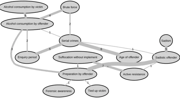
Starting with the node “Preparation of offender”, which is defined as the level of preparation to gain control over the victim, to hide the crime and to conduct the sexual assault, we observe 6 edges. The node may be located in the fourth row from below to the right in Figure 9 or in the lower centre of Figure 4. Of the emerging edges from the node “Preparation of offender”, the edge towards the node
“Sadistic Offender” sticks out by its thickness. The state of this node is defined via the psychiatric examination of the offender and is clearly connected to sadistic ac- tions by the offender during the crime, included as the node “Sadism” in the graph.
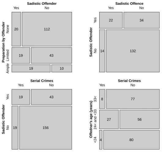
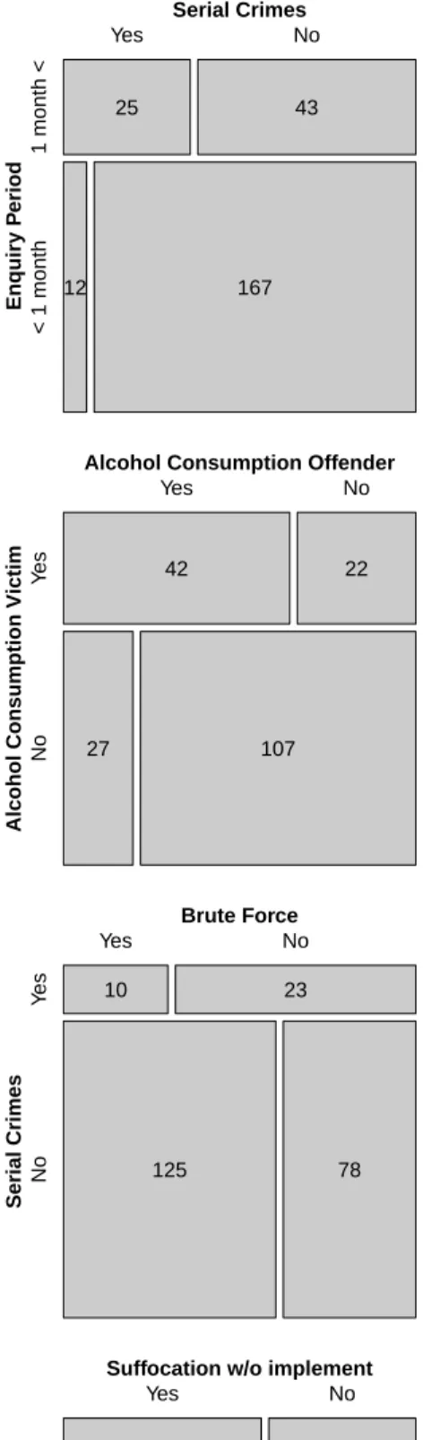
Examining the corresponding mosaic plots in Figure 6 it may be concluded that a sadistic offender is much more likely to behave sadistically and shows a higher level of preparation. Furthermore a sadistic offender conducts serial crimes more often than a non–sadistic offender. The node “Serial crimes”, a dummy variable indicating if the specific crime is part of a wider series, exhibits profound edges to the offender’s age and the enquiry period. Serial criminals usually belong to an age group of 24 to 33 years and obviously such a crime carries a longer enquiry period, as depicted in the mosaic plot in Figure 7.
Apart from the sadistic offender, the serial criminal marks the second ideal ex- ample of an offender driven crime. On the other hand, there are situation driven crimes. These crimes show low levels of organisation by the offender and for the most part do not involve neither sadistic nor serial criminals. Rather they display a strong influence of the consumption of alcohol, which can be read in the graph by the edge between “Preparation by offender” and the node “Alcohol consumption by offender”. This negative interaction is expanded by the node “Alcohol consump- tion by the victim” stating if the victim had consumed alcohol before the offender’s attack. These also include cases in which the offender and victim voluntary and be- fore the offender’s attack engage in drinking. Most often either the victim and the offender have both consumed alcohol, which often leads to a situation driven crime, or neither the victim nor the offender have consumed alcohol, which characterises an offender driven crime. Apart from alcohol, the situation driven crimes are also
1 2 3 4 5 6 7 8
Algorithms indicating same edge Frequency of edges 051015202530
Figure 3: Bar chart stating how many algorithms indicate the same edge and the frequency of such edges
Alcohol consumption by victim Brute force
Alcohol consumption by offender
Suffocation without implement Serial crimes
Age of offender
Sadism
Sadistic offender
Preparation by offender
Forensic awareness Tied up victim
Enquiry period
Active resistance
4 4
2 1
3 2
1 4
6 1
5 5
7 1
1 1
Figure 4: Excerpt of Figure 9 showing variables which mark the difference between an offender and situation driven crime
marked by the use of brute force by the offender to gain and maintain control over the victim. The graphical model illustrates this interaction by the edge between
“Alcohol consumption by offender” and the node “Brute force”, which reflects any injuries of the victim due to the application of blunt force.
Serial criminals with their high level of preparation generally do not rely on blunt force, but apply more sophisticated measures to control the victim. This negative interaction can be read off the cross–table corresponding to the edge between “Brute force” and “Serial crimes”. One such measure to control the victim applied by of- fenders in a criminal driven crime is described by the edge between “Preparation by offender” and the node “Tied up victim”. This node indicates if the victim is tied up by the offender and the corresponding cross–table reveals that offenders characterised by a high level of preparation are more likely to tie up their victim.
Furthermore these offenders suffocate their victims less often with their hands, as highlighted by the cross–table corresponding to the edge between “Preparation by offender” and “Suffocation without implement”. In general criminals with a high level of preparation apply a more instrumental mode to gain and maintain con- trol, whereas a low level of preparation leads to a more expressive crime, where the offender likely applies blunt force. However, the likelihood of suffocation by the offender rises in both cases, whenever the victim strongly resists the attack.
This general influence of the victim on the crime is specified by the edge between the nodes “Suffocation without implement” and “Active resistance”, where active resistance is defined as resisting the assault physically, trying to escape or calling for help. The corresponding mosaic plot on this interaction is given in Figure 8.
During the crime the level of planing carries over to the criminals’ behaviour, as a high level of planing is accompanied by a high level of forensic awareness. Foren- sic awareness describes measures to hide the crime by for example using gloves or cleaning the crime scene afterwards. The corresponding node “Forensic awareness”
is connected to the node “Planing by offender” highlighting this positive interaction.
Enquiry period Offender victim relationship
Distance: hub−contact location
Contact location
Forensic awareness
Movement of corpse
Different assault location
4 3
4 4
1 5
5
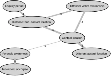
Figure 5: Excerpt of Figure 9 showing geographical variables and their adjacency which mark the difference between an offender and situation driven crime
The node “Forensic awareness” links the degree of planning by the offender to cer- tain geographical characteristics of the crime. The node may be found on the third row from below to the right in Figure 9 or to the left in Figure 5. Firstly, a criminal showing a high level of forensic awareness is more likely to hide the corpse at a separate location which serves solely for this purpose and complicates the prosecu- tion. This interaction is reflected by the edge between “Forensic awareness” and
“Movement of corpse”. Furthermore the node “Forensic awareness” is connected to the node “Contact location”. This node describes the location of the first contact between the offender and the victim before the assault and distinguishes between location indoors, such as the victim’s flat, the offender’s flat or a shared flat, and locations outdoors.
The corresponding mosaic plot reveals that offenders are less likely to show a high level of forensic awareness, if the contact takes place in their familiar surroundings, e.g. their own or a shared flat. On the contrary offenders meeting the victim in a rather unknown surrounding like the victim’s flat or some location outdoors show a high level of forensic awareness and the corresponding crime is therefore most likely offender driven. The node “Contact location” exhibits a profound edge to the node
“Offender victim relationship”, which details the pre–attack relationship between the offender and the victim. Examining the corresponding cross–table reveals that the contact between the offender and an unknown victim is mostly established out- doors, whereas offenders meet any known victims rather indoors.
As an outdoor location is associated with a high level of forensic awareness, these outdoors contacts between the offender and the unknown victim may be attributed to the offender driven crime, whereas the indoor contact exhibits the characteristics of a situation driven crime and likely includes a victim known to the offender. An offender meeting the victim in his familiar surrounding obviously does not travel a great distance from his personal hub to the contact location, where a hub is defined as any location the offender is perfectly familiar with, e.g. his flat or work place.
The graph therefore includes an edge between these two nodes. Furthermore the node “Distance: hub – contact location” is connected to the node “Enquiry period”
and the corresponding cross–table details that a greater distance between the of- fender’s personal hub and the contact location complicates the prosecution, as the enquiry period rises.
In general, it may be concluded, that the differentiation between an offender driven crime and a situation driven crimes carries over to the geographical variables. Well organised offenders meet the victim in general not in their familiar surrounding, but have rather travelled a longer distance and hide the corpse at a separate location to impede the exposure of their crime. Less organised offenders meet the victim, which is most likely known to them, in rather familiar surroundings and do not travel a great distance. Furthermore they do not show a high level of forensic awareness or hide the corpse at a separate location. However, as before, the actual crime is not solely influenced by the criminal, as an examination of the edge between the nodes
“Contact location” and “Different assault location” depicts. If the offender meets the victim in an outdoors location, in just over half of the crimes, the ensuing attack is conducted at a different location. The offender may not feel confident, that the contact location outdoors allows him to conduct the crime and is therefore forced to the change the location. This change of location occurs only in less of a quarter of all crimes, in which the contact location is indoors.
5 Discussion
This study demonstrates that learning a BN from data yields several insights into the domain of sex–related homicides. Hence we provide profilers with profound knowledge and extend previous statistical research in the realm of offender profiling.
The combined skeleton of the obtained BNs shows the dependency structure in the domain and is calculated via various algorithms. The resulting single BNs of these algorithms are combined to a final structure by summing up on how often an edge is found by the diverse algorithms. This number is interpreted as a confidence mea- sure in the actual existence of the corresponding dependency in the data generating process. The algorithms are applied on a new data set of 252 cases of sex–related homicides in Germany. This data was collected using a tedious process of reading prosecutor’s files and defining appropriate variables via Comparative Text Analysis.
In general, a notional scale with two oppositional prototypes of sex–related homi- cides and several increments in between can be deduced from the graphical model.
On one hand several criminals show a high level of preparation and forensic aware- ness. They apply sophisticated measures to control the victim and are more likely to exhibit a sadistic or serial background. Furthermore, they more often attack vic- tims unknown to them, which they contact in unfamiliar surroundings. These crimes carry a rather long enquiry period. On the other hand, several criminals do not show high levels of preparation or forensic awareness. Instead alcohol often constitutes a vital part of the crime and the offenders are more likely to apply blunt force instead of more elaborated measures to control the victim. They are often known to the victim and act in familiar surroundings. Several investigated crimes do not belong strictly to one of these prototypes, but exhibit only some of the specified features or even show features of both prototypes. However, in any case offenders have to interact with factors, which they cannot affect, like the victim’s resistance or the characteristics of the contact location. These and other variables mirror the applied Criminal Event Perspective, which states that the actions on the crime scene are determined simultaneously by the offender, the victim and the underlying situation.
The distinction between an offender and situation driven crime examines the graph- ical model in a certain perspective. Different views exist to analyse sex–related homicides and consequently different distinctions may be found. However, due to the low number and the heterogeneity of the analysed cases these points of view do not stick out as clearly as the described distinction, but have been noticed in smaller sub–samples (Safarik et al., 2002). More data would be necessary to reveal them in the proposed general graphical model. But sex–related homicides occur rarely and it may therefore be infeasible to obtain a larger sample.
In the meantime a BN based on the presented skeleton reveals promising prediction results. For example in an extensive series in northern Germany of a masked man conducting single sexual assaults on boys over several years and confessing the mur- der of three of them recently, the age group of the offender is predicted correctly by the BN. The offender being 30 years old at the time of his last admitted murder, is classified correctly in the middle age group of being older than 24, but younger than 33 based on known facts at the time of that crime. Taking into account that the presented skeleton primary serves as describing the dependence structure in the domain of sex–related homicides, the application of prediction techniques based on the presented results in this study poses a natural next step in the analysis of sex–related homicides.
Sadistic Offender
Preparation by Offender AmpleLimitedNone
Yes No
20 112
19 43
19 10
Sadistic Offence
Sadistic Offender NoYes
Yes No
22 34
14 132
Serial Crimes
Sadistic Offender NoYes
Yes No
19 43
19 156
Serial Crimes
Offedner's age (years) <2424< and <3333<
Yes No
8 77
27 56
4 80
Figure 6: Mosaic plots corresponding to discussed edges
Serial Crimes
Enquiry Period < 1 month1 month <
Yes No
25 43
12 167
Alcohol Consumption Offender
Preparation by Offender AmpleLimitedNone
Yes No
59 77
12 47
1 26
Alcohol Consumption Offender
Alcohol Consumption Victim NoYes
Yes No
42 22
27 107
Alcohol Consumption Offender
Brute Force NoYes
Yes No
55 73
19 73
Brute Force
Serial Crimes NoYes
Yes No
10 23
125 78
Tied up Victim
Preparation by Offender AmpleLimitedNone
Yes No
30 104
20 44
17 12
Suffocation w/o implement
Preparation by Offender AmpleLimitedNone
Yes No
78 58
22 37
8 18
Forensic Awareness
Preparation by Offender AmpleLimitedNone
Ample Limited None
16 61 47
10 32 13
11 8 3
Figure 7: Mosaic plots corresponding to discussed edges
Suffocation w/o implement
Active Resistance NoYes
Yes No
85 67
12 38
Forensic Awareness
Movement of Corpse NoYes
Ample Limited None
18 27 3
19 82 64
Contact Location
Forensic Awareness NoneLimitedAmple
Familiar Unfamiliar
4 32
7 99
22 44
●
Contact Location
Distance: Hub − Contact Location (km) 10<1< and >10<1
Familiar Unfamiliar
35 89
2 58
48
Distance: Hub − Contact Location (km)
Enquiry Period (month) < 11 <
<1 1< and >10 10<
13 21 26
110 39 23
Contact Location
Different Assault Location NoYes
Indoors Outdoors
40 55
108 44
Contact Location
Offender Victim Realtion UnknownKnown
Indoors Outdoors
115 38
30 58
Figure 8: Mosaic plots corresponding to discussed edges
Suffocation with implement Brute force Suffocation without implement
Gender of victim Nationality of victim
Age of victim Number of offendersEnquiry period
Alcohol consumption by victim Alcohol consumption by offender
Provocation: insult
Provocation: financial dispute Provocation: Sex. demands Provocation: break−up
Intention of robbery Consensual sex Prostitution Preparation by offender Forensic awareness
Disguised identity
Robbery Active resistance
Passive resistance Threat Tied up victim
Deception Anal intercourse
Demand sex. acts Fellatio Inserted finger Kissing Sadism Vaginal intercourse
Intercourse with corpse
Sex. manipulation of corpseOffender victim relationship Appraisal of diminished responsibility
Serial crimes Sadistic offender
Sex. frustration Age of offender Offender: permanent relationship
Criminal record: violence Criminal record: sex offences
Criminal record: against property Offender: criminal environment Offender: socially marginalisedOffender: social isolation
Crucial personal circumstances Distance: hub−contact location Contact location Different assault location
Movement of corpse
25 4 2 14
1 1 2
2 7
4 1 1
2 1 3
322 5
12 4
8
13 1 3
1
17
2 7
8 3 11 1 4
117 15
2
21
3 1
7 1 2
1 2 2
7 2 6
7 5 3
1
43 4
71
61 44 341
8
8 1 1
2 4 4 5 Figure9:GraphicalModelforsex–relatedhomicides.Numbersontheedgesdenotehowmanyalgorithmsdetecttheparticularedge.
References
Aitken, C. G. G., Gammerman, A., Zhang, G., Connolly, T., Bailey, D., Gordon, R.
and Oldfield, R. (1996). Bayesian belief networks with an application in specific case analysis. In Computational Learning and Probabilistic Reasoning (ed A.
Gammerman). Chichester: Wiley.
Aliferis, C. F., Tsamardinos, I. and Statnikov, A. (2003). HITON, a novel Markov blanket algorithm for optimal variable selection. InProceedings of the 2003 Amer- ican medical informatics Association Annual Symposium, 21–25.
Alison, L. , Bennell, C., Mokros, A. and Ormerod, D. (2002). The personality paradox in offender profiling Psychology, Public Policy, and Law,8, 115–135.
Baumgartner, K., Ferrari, S. and Palermo, G. (2008). Constructing Bayesian Net- works for Criminal Profiling from Limited Data. Knowledge–Based Systems,21, 563–572.
Beauregad, ´E. (2007). The Role of Profiling in the Investigation of Sexual Homi- cide. In Sexual Murderers: A Comparative Analysis and New Perspectives (eds J. Proulx, ´E. Beauregard, M. Cusson and A. Nicole). Chichester: Wiley.
Cheng, J., Greiner, R., Kelly, J., Bell, D. A. and Liu, W. (2002). Learning Bayesian Networks from data. The Artificial Intelligence Journal,137, 43–90.
Chickering, D. M. (1996). Learning Bayesian Networks is NP–complete. InLearning from Data: Artificial Intelligence and Statistics V (eds Fisher, D. and Lenz, H.–
J.). New York: Springer.
Chipman, H. A., George, E. I. and McCulloch, R. E. (1998). Bayesian CART model search. Journal of the American Statistical Association,93, 935–948.
Davies, A. (1997). Specific profile analysis: a data–based approach to offender profiling. In Offender profiling: Theory, Research and Practise (eds Jackson, J.
L. and Bekerian, D. A.). Chichester: Wiley.
Fleiss, J. L. (1971). Measuring nominal scale agreement among many raters. Psy- chological Bulletin,76, 378–382.
Friedman, N., Linial, M., Nachman, I. and Peer, D. (2000). Using Bayesian Networks to Analyze Expression Data. Journal of Computational Biology,7, 601–620.
Friedman, N., Nachman, I. and Peer, D. (1999). Learning Bayesian Network Struc- ture from massive Datasets. Proceedings of the Fifteenth Conference on Uncer- tainty in Artificial Inteligence, 206–215.
Heckerman, D. (1990). Probabilistic similarity networks. Networks,20, 607–636.
Jensen, F. V. (1996). Introduction to Bayesian Networks. New York: Springer.
Kalisch, M. and B¨uhlmann, P. (2007). Estimating high–dimensional directed acyclic graphs with the PC–Algorithm. Journal of Machine Learning Research,8, 613–
636.
Lauritzen, S. L., Dawid, A. P., Larsen, B. N. and Leimer, H. G. (1990). Independence properties of directed markov fields. Networks,20, 491–505.
Lauritzen, S. L. (1996). Graphical Models. Oxford: Clarendon Press.
Li, J. and Wang, Z. J. (2009). Controlling the false discovery rate of the associ- ation/causality structure learned with the PC algorithm. Journal of Machine Learning Research,10, 475–514.
Margaritis D. and Thrun, S. (1999). Bayesian Network induction via local neigh- borhoods. In Advances in Neural Information Processing Systems 12 (eds Solla, S. A., Leen, T. K. and M¨uller, K.–R.). Cambridge: MIT Press.
Meinshausen, N. and B¨uhlmann, P. (2006). High–Dimensional graphs and variable selection with the LASSO. The Annals of Statistics,34, 1436–1462.
Miethe, T. D. and Regoeczi, W. C. (2004). Rethinking Homicide. New York:
Cambridge University Press.
Mokros, A. and L. J. Alison (2002). Is offender profiling possible? Legal and Criminological Psychology,7, 25–43.
Pearl, J. (2000). Causality. New York: Cambridge University Press.
Ressler, R. K., Burgess, A. W. and Douglas, J. E. (1988). Sexual homicide. New York: Lexington Books.
Robinson, R. W. (1977). Counting unlabelled acyclic digraphs. InLecture Notes in Mathematics: Combinatorial Mathematics V. Heidelberg: Springer.
Safarik, M. E., Jarvis, J. P. and Nussbaum, K. E. (2002). Sexual Homicide of Elderly Females. Journal of Interpersonal Violence,17, 500–525
Salfati, G. and Canter, D. V. (1999). Differentiating stranger murders: profiling offender characteristics from behavioral styles. Behavioral Scinces and the Law, 17, 391–406.
Sprites, P., Glymour, C. and Scheines, R. (2000). Causation, prediction and Search.
Cambridge: MIT Press.
Strauss, A. and Corbin, J. M. (1990). Basics of qualitative research. Thousand Oaks: Sage Publications.
Tausendteufel, H., Stahlschmidt, S. and K¨uhnel, W. (2011).Bestimmung des T¨ater- alters bei sexuell assoziierten T¨otungsdelikten auf der Basis von Tatgeschehens- merkmalen. Wiesbaden: Bundeskriminalamt.
Tsamardinos, I., Aliferis, C. F. and Statnikov, A. (2003). Algorithms for large scale markov blanket discovery. In The 16th International FLAIRS Conference, 376–381.
Tsamardinos, I., Brwon, L. E. and Aliferis, C. F. (2006). The max–min hill–climbing Bayesian Network structure learning algorithm. Machine Learning,65, 31–78.
Verma, T. and Pearl, J. (1990). Equivalence and synthesis of causal models. In Proceedings of the Sixth Conference on Uncertainty in Artificial intelligence, 220–
227.
Wright, S (1921). Correlation and Causation. Journal of Agricultural Research,20, 558–585.
Zuk, O., Margel, S. and Domany, E. (2006). On the number of samples needed to learn the correct structure of a Bayesian Network. InUAI 2006.
SFB 649 Discussion Paper Series 2011
For a complete list of Discussion Papers published by the SFB 649, please visit http://sfb649.wiwi.hu-berlin.de.
001 "Localising temperature risk" by Wolfgang Karl Härdle, Brenda López Cabrera, Ostap Okhrin and Weining Wang, January 2011.
002 "A Confidence Corridor for Sparse Longitudinal Data Curves" by Shuzhuan Zheng, Lijian Yang and Wolfgang Karl Härdle, January 2011.
003 "Mean Volatility Regressions" by Lu Lin, Feng Li, Lixing Zhu and Wolfgang Karl Härdle, January 2011.
004 "A Confidence Corridor for Expectile Functions" by Esra Akdeniz Duran, Mengmeng Guo and Wolfgang Karl Härdle, January 2011.
005 "Local Quantile Regression" by Wolfgang Karl Härdle, Vladimir Spokoiny and Weining Wang, January 2011.
006 "Sticky Information and Determinacy" by Alexander Meyer-Gohde, January 2011.
007 "Mean-Variance Cointegration and the Expectations Hypothesis" by Till Strohsal and Enzo Weber, February 2011.
008 "Monetary Policy, Trend Inflation and Inflation Persistence" by Fang Yao, February 2011.
009 "Exclusion in the All-Pay Auction: An Experimental Investigation" by Dietmar Fehr and Julia Schmid, February 2011.
010 "Unwillingness to Pay for Privacy: A Field Experiment" by Alastair R.
Beresford, Dorothea Kübler and Sören Preibusch, February 2011.
011 "Human Capital Formation on Skill-Specific Labor Markets" by Runli Xie, February 2011.
012 "A strategic mediator who is biased into the same direction as the expert can improve information transmission" by Lydia Mechtenberg and Johannes Münster, March 2011.
013 "Spatial Risk Premium on Weather Derivatives and Hedging Weather Exposure in Electricity" by Wolfgang Karl Härdle and Maria Osipenko, March 2011.
014 "Difference based Ridge and Liu type Estimators in Semiparametric Regression Models" by Esra Akdeniz Duran, Wolfgang Karl Härdle and Maria Osipenko, March 2011.
015 "Short-Term Herding of Institutional Traders: New Evidence from the German Stock Market" by Stephanie Kremer and Dieter Nautz, March 2011.
016 "Oracally Efficient Two-Step Estimation of Generalized Additive Model"
by Rong Liu, Lijian Yang and Wolfgang Karl Härdle, March 2011.
017 "The Law of Attraction: Bilateral Search and Horizontal Heterogeneity"
by Dirk Hofmann and Salmai Qari, March 2011.
018 "Can crop yield risk be globally diversified?" by Xiaoliang Liu, Wei Xu and Martin Odening, March 2011.
019 "What Drives the Relationship Between Inflation and Price Dispersion?
Market Power vs. Price Rigidity" by Sascha Becker, March 2011.
020 "How Computational Statistics Became the Backbone of Modern Data Science" by James E. Gentle, Wolfgang Härdle and Yuichi Mori, May 2011.
021 "Customer Reactions in Out-of-Stock Situations – Do promotion-induced phantom positions alleviate the similarity substitution hypothesis?" by Jana Luisa Diels and Nicole Wiebach, May 2011.
SFB 649, Ziegelstraße 13a, D-10117 Berlin http://sfb649.wiwi.hu-berlin.de This research was supported by the Deutsche
SFB 649 Discussion Paper Series 2011
For a complete list of Discussion Papers published by the SFB 649, please visit http://sfb649.wiwi.hu-berlin.de.
022 "Extreme value models in a conditional duration intensity framework" by Rodrigo Herrera and Bernhard Schipp, May 2011.
023 "Forecasting Corporate Distress in the Asian and Pacific Region" by Russ Moro, Wolfgang Härdle, Saeideh Aliakbari and Linda Hoffmann, May 2011.
024 "Identifying the Effect of Temporal Work Flexibility on Parental Time with Children" by Juliane Scheffel, May 2011.
025 "How do Unusual Working Schedules Affect Social Life?" by Juliane Scheffel, May 2011.
026 "Compensation of Unusual Working Schedules" by Juliane Scheffel, May 2011.
027 "Estimation of the characteristics of a Lévy process observed at arbitrary frequency" by Johanna Kappus and Markus Reiß, May 2011.
028 "Asymptotic equivalence and sufficiency for volatility estimation under microstructure noise" by Markus Reiß, May 2011.
029 "Pointwise adaptive estimation for quantile regression" by Markus Reiß, Yves Rozenholc and Charles A. Cuenod, May 2011.
030 "Developing web-based tools for the teaching of statistics: Our Wikis and the German Wikipedia" by Sigbert Klinke, May 2011.
031 "What Explains the German Labor Market Miracle in the Great Recession?" by Michael C. Burda and Jennifer Hunt, June 2011.
032 "The information content of central bank interest rate projections:
Evidence from New Zealand" by Gunda-Alexandra Detmers and Dieter Nautz, June 2011.
033 "Asymptotics of Asynchronicity" by Markus Bibinger, June 2011.
034 "An estimator for the quadratic covariation of asynchronously observed Itô processes with noise: Asymptotic distribution theory" by Markus Bibinger, June 2011.
035 "The economics of TARGET2 balances" by Ulrich Bindseil and Philipp Johann König, June 2011.
036 "An Indicator for National Systems of Innovation - Methodology and Application to 17 Industrialized Countries" by Heike Belitz, Marius Clemens, Christian von Hirschhausen, Jens Schmidt-Ehmcke, Axel Werwatz and Petra Zloczysti, June 2011.
037 "Neurobiology of value integration: When value impacts valuation" by Soyoung Q. Park, Thorsten Kahnt, Jörg Rieskamp and Hauke R.
Heekeren, June 2011.
038 "The Neural Basis of Following Advice" by Guido Biele, Jörg Rieskamp, Lea K. Krugel and Hauke R. Heekeren, June 2011.
039 "The Persistence of "Bad" Precedents and the Need for Communication:
A Coordination Experiment" by Dietmar Fehr, June 2011.
040 "News-driven Business Cycles in SVARs" by Patrick Bunk, July 2011.
041 "The Basel III framework for liquidity standards and monetary policy implementation" by Ulrich Bindseil and Jeroen Lamoot, July 2011.
042 "Pollution permits, Strategic Trading and Dynamic Technology Adoption"
by Santiago Moreno-Bromberg and Luca Taschini, July 2011.
043 "CRRA Utility Maximization under Risk Constraints" by Santiago Moreno- Bromberg, Traian A. Pirvu and Anthony Réveillac, July 2011.
SFB 649, Ziegelstraße 13a, D-10117 Berlin http://sfb649.wiwi.hu-berlin.de
SFB 649 Discussion Paper Series 2011
For a complete list of Discussion Papers published by the SFB 649, please visit http://sfb649.wiwi.hu-berlin.de.
044 "Predicting Bid-Ask Spreads Using Long Memory Autoregressive Conditional Poisson Models" by Axel Groß-Klußmann and Nikolaus Hautsch, July 2011.
045 "Bayesian Networks and Sex-related Homicides" by Stephan Stahlschmidt, Helmut Tausendteufel and Wolfgang K. Härdle, July 2011.
SFB 649, Ziegelstraße 13a, D-10117 Berlin http://sfb649.wiwi.hu-berlin.de This research was supported by the Deutsche