Unlocking the potential of biological sample archives:
benthic-pelagic feeding of Baltic cod assessed by otolith protein amino-acid specific stable isotope analysis
Bachelorarbeit
im Ein-Fach-Bachelorstudiengang Biologie der Mathematisch-Naturwissenschaftlichen Fakultät
der Christian-Albrechts-Universität zu Kiel
vorgelegt von
Paulina Urban
Erstgutachter: Prof. Dr. Hinrich Schulenburg Zweitgutachter: Dr. Jan Dierking Drittgutachter: Dr. Thomas Larsen
Kiel im Dezember 2016
Drawing: Jonas Mölle
I
TABLE OF CONTENTS
TABLE OF CONTENTS... I LIST OF TABLES ... II LIST OF FIGURES ... III LIST OF ABBREVIATIONS ... IV
ZUSAMMENFASSUNG ... 1
ABSTRACT ... 3
INTRODUCTION ... 4
MATERIAL AND METHODS ... 10
Study area ... 10
Study organism ... 11
Sampling ... 12
Sampling design ... 12
Sample Preparation ... 14
Extraction the organic matrix out of otoliths ... 14
Muscle samples ... 15
Stable isotope analysis (SIA) ... 16
Principle of bulk stable isotope analysis (bulk SIA) ... 16
Stable isotope analysis of samples ... 18
Principle of compound-specific stable isotope analysis (CSIA for 13CAA) ... 18
Sample Preparation and Analysis for CSIA ... 19
RESULTS ... 21
Relationship of otolith length / weight and cod individual data ... 21
bulk SIA ... 22
Method applicability testing ... 22
How do bulk SIA values (C, N, S) differ between muscle tissue and otolith protein of the same cod individual? ... 22
II How strongly do bulk SIA values differ between otolith protein from left and right
otoliths of the same fish? ... 24
Biological case study ... 26
Cod in context of prey ... 26
How strongly do cod individuals differ in isotopic values? ... 30
CSIA ... 31
Method applicability testing ... 31
How do CSIA (C) values differ between muscle tissue and otolith protein? ... 31
Cod in context of prey ... 33
DISCUSSION ... 34
Otolith protein bulk and compound-specific SIA method feasibility ... 34
Assessment of benthic vs. pelagic feeding of cod ... 38
Caveats, lessons and next steps (bulk SIA and CSIA) ... 39
Approach towards long-term reconstruction of cod’s benthic vs. pelagic feeding ... 40
REFERENCES ... 41
ACKNOWLEDGMENTS ... 45
ERKLÄRUNG ... 46
LIST OF TABLES Table 1. Comparison of 15N, 13C, 34S isotope values. ... 23
Table 2. Comparison of 15N, 13C, 34S isotope values. ... 23
Table 3. Summary of the linear relationship and regression values ... 23
Table 4. Summary of the bulk SIA values of right and left otolith proteins. ... 26
Table 5. Summary of mean isotope values ... 30
III
LIST OF FIGURES
Figure 1. The Baltic Sea is a large brackish sea. ... 4
Figure 2. Gadus morhua, the Baltic’s top predator fish. ... 5
Figure 3. Schematic description of the cod’s feeding ecology. ... 6
Figure 4. Pair of otoliths (sagittae) of Gadus morhua ... 6
Figure 5. Graph of the decline of the eastern Baltic cod population ... 7
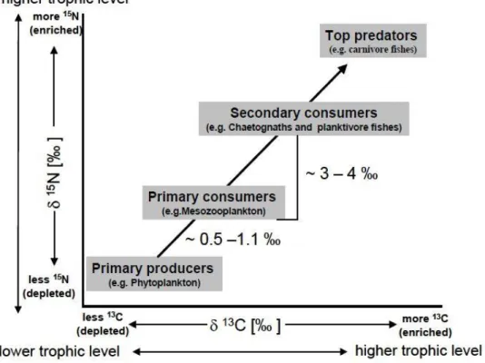
Figure 6. Schematic plot of 13C and 15N isotope. ... 8
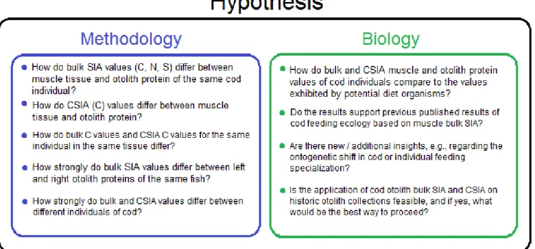
Figure 7. Hypotheses of this study presented as questions... 10
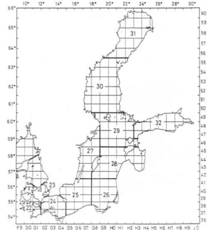
Figure 8. Baltic Sea divided in subdivisions (SD) ... 11
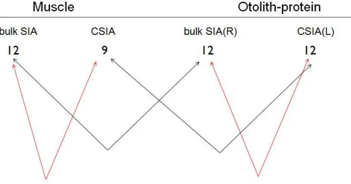
Figure 9. Sampling design for the methodology part. ... 13
Figure 10. Diagram of the different steps for sample preparation. ... 17
Figure 11. Reults of length, width and mass measurements of the cod otoliths. ... 21
Figure 12. Comparison of 15N, 13C, 34S isotope values ... 22
Figure 13. Linear relationship of otolith protein and muscle stable isotope values of Baltic cod. ... 24
Figure 14. Individual value plots for a comparison between left and right otolith proteins. ... 25
Figure 15. Individual value plots comparing left and right otolith proteins ... 25
Figure 16. Comparison of 15N, 13C , 34S isotope values. ... 27
Figure 17. Boxplot of 15N isotope value of all analysed Baltic-organisms... 28
Figure 18. Boxplot of 13C isotope value of all analysed Baltic-organisms ... 28
Figure 19. Boxplot of 34S isotope value of all analysed Baltic-organisms. ... 29
Figure 20. Biplot of mean nitrogen (15N) and sulfur (34S) values of all analysed species before conversion of the otolith protein values ... 29
Figure 21. Biplot of mean nitrogen (15N) and sulfur (34S) values of all analysed species after conversion of the otolith protein values ... 30
Figure 22. Diagram to visualise the lack of an ontogenetic shift. ... 31
Figure 23. Principal component analysis of 13CAA patterns of different organisms of the Baltic Sea ... 32
Figure 24. Linear discriminant analysis based on the 13C AA patterns of different organisms of the Baltic Sea ... 32
IV
LIST OF ABBREVIATIONS
delta
AA amino acid
Ala alanine
Asx asparagine
BB Bornholm Basin
C carbon
CSIA Compound-Specific Stable Isotope Analysis
EAA essential amino acid
Glx glutamine
Gly glycine
His histidine
ICES International Council for the Exploration of the Sea
Ile isoleucine
ISOM insoluble organic material
JFT Jungfischtrawl
L Carl von Linné
LDA Linear Discriminant Analysis
LD1/LD2 linear discriminant 1/ linear discriminant 2
Leu leucine
Lys lysine
MD mean difference
Met methionine
N nitrogen
n samples size
p p-Value
psu particle salinity units
PCA Principal Component Analysis
PC1/PC2 principal component 1/ principal component 2
Phe phenylalanine
S sulfur
SCA Stomach Content Analysis
SD Subdivision
sd standard deviation
SIA Stable Isotope Analysis
SOM soluble organic material
Thr threonine
TL total length
Tyr tyrosine
Val valine
1
Zusammenfassung
Langzeitreihen sind wichtige Werkzeuge der Ökologen und werden eingesetzt, um Ökosystemveränderungen zu erklären. Da solche Datenreihen selten sind, wurden Methoden entwickelt, die rückblickend Analysen und die Rekonstruktion von Lang- zeitreihen ermöglichen. Otolithen sind Verknöcherungen im Innenohr von Fischen.
Diese Strukturen werden seit Jahrhunderten in Museen und Forschungseinrichtun- gen gesammelt, da sie traditionell in Alterslesungen eingesetzt werden. Kürzlich wur- de gezeigt, dass Otolithen potenziell eingesetzt werden können, um das Beutespekt- rum von Fischen zu rekonstruieren, was jedoch methodisch nicht einfach ist. In mei- ner Arbeit habe ich deshalb eine Kombination von zwei potentiell vielversprechenden Verfahren zur retrospektiven Analyse von Fischnahrung an den Otolithen von 12 Ostseedorschen (Gadus morhua), beprobt im Bornholmbecken, getestet: 1) stabile Isotopen Analyse am gesamten Gewebe (bulk SIA) mittels 13C, 15N, 34S und 2) Komponenten-spezifische stabile Isotopen Analyse (CSIA). Bei der CSIA werden aus dem zu untersuchenden Gewebe einzelne Komponenten, wie zum Beispiel die Ami- nosäuren (AA), extrahiert und einzeln analysiert, was die Auflösung von Ergebnissen im Vergleich zu bulk SIA Ergebnissen erhöhen kann. Bezüglich 1) bulk SIA erwies sich – auch wegen der besseren Verfügbarkeit von Rahmendaten von potenziellen Beuteorganismen – als die in der Ostsee momentan aussagekräftigere Methode für die retrospektiven Ernährungsanalysen von Fischen. Der Vergleich der Isotopenwer- te der Otolithenprotein-Fraktionen mit den üblicherweise in Isotopenstudien verwen- deten Muskelgewebeproben zeigte systematische und deshalb vorhersagbare Ver- schiebungen. Diese Verschiebungen spielen eine Schlüsselrolle für die Interpretation von Isotopenwerten der Otolithenproteine, wodurch die Anwendung der Verschie- bungen auf die Isotopenwerte der Otolithenproteine theoretische Muskel- Isotopenwerte berechnet werden können, die anschließend mittels etablierter Inter- pretationsansätze für Muskel-Isotopenwerte gedeutet werden können. Hier zeigte die Interpretation der theoretischen bulk SIA Muskelwerte im Rahmen von Isotopenwer- ten möglicher Nahrungsquellen, dass die untersuchten Dorsche sich unabhängig von ihrer Größe pelagisch ernährten, d.h., ein benthisch-pelagischer ontogenetischer Nahrungs-Shift war nicht zu erkennen. Bezüglich 2), CSIA Resultate von essentiellen Aminosäuren im Otolithenprotein und in Muskelgewebe desselben Fisches waren
2 vergleichbar. Die Interpretation dieser Werte im Rahmen von – im Umfang begrenz- ten – Informationen zu möglichen Nahrungsquellen bestätigte teilweise die Bedeu- tung pelagischer Nahrung für Dorsch, wies aber auch auf eine potenziell in der Ana- lyse fehlende Nahrungsquelle hin. Diese Studie unterstreicht das Potenzial der stabi- len Isotopenanalyse von Otolithenproteinen für die Rekonstruktion der Nahrungsöko- logie von Fischen und bildet das Fundament für die zukünftige Rekonstruktion von Langzeitdatenreihen zur Bedeutung benthischer vs. pelagischer Nahrung für den Ostseedorsch.
3
Abstract
Ecologists often rely on long-term data series to explain and predict environmental change. Although such data sets are rare, records of past changes can be produced retroactively from materials such as otoliths, the inner ear structures or fish, archived in museums collections. These otoliths are formed over the life-time of a fish and are metabolically inert, and therefore sometimes considered a “black box” containing in- formation about a fish’s life. It can, however, be methodologically challenging recon- structing fish diets from otolith records. Here, in order to test the feasibility of the method, and to gain information about the feeding ecology of Baltic cod (Gadus morhua) from conserved otoliths, we applied a combination of two different stable isotope techniques to the protein component of otoliths of cod sampled in Bornholm Basin: 1) bulk stable isotope analysis (bulk SIA) on 13C, 15N, 34S isotopes and 2) compound specific stable isotope analysis (CSIA), which provides data on single compounds such as individual amino acids (AA) rather than total tissue and can en- hance the resolution and improve differentiation between different food sources. Re- garding 1), due to the currently better availability of diet framework data, we estimat- ed the bulk stable isotope analysis to be the more powerful one for diet reconstruc- tion purposes in the Baltic Sea. Bulk SIA comparison between otolith protein fractions and the traditionally used muscle tissue showed systematic and highly predictable shifts. These shifts played a key role for the interpretation of otolith protein isotope values. The application of our estimated shifts on the otolith protein isotope values resulted in theoretical muscle bulk isotope values, for which interpretation for feeding ecology purposes is established. Interpretation of these values in a framework of bulk SIA values of cod’s potential prey indicated that Bornholm Basin cod showed an al- most exclusively pelagic diet with no benthic - pelagic diet shift. Regarding 2), CSIA of essential amino acids yielded comparable results for otolith protein and muscle tissue of the same fish. CSIA results interpreted in a more limited framework of po- tential diet values in part confirmed the pelagic diet of cod, but also pointed to poten- tial missing diet sources in the analysis. This study confirmed the potential of otoliths for retrospective analyses of the diet of fish and provides the foundation for the re- construction of long-term data series in cod feeding ecology in the Baltic Sea using archived otolith collections.
4
Introduction
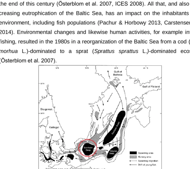
Ecosystems worldwide are affected by global change (Walther et al. 2002). The re- sulting changes in environmental conditions of sea and oceans include temperature increase (Levitus et al. 2000) and ocean acidification (Fabry et al. 2008). In addition, global change affects individual organisms, which results in fish migration (Walther et al. 2002) and whole organism communities changing their structure and functioning within ecosystems (Hoegh-Guldberg & Bruno 2010). The Baltic Sea (Fig. 1.) is one of the best known examples of an ecosystem where conditions for living organisms are getting more and more extreme influencing the organism’s interactions (Österblom et al. 2007).
The Baltic Sea is one of the world’s largest brackish water reservoirs and a semi- enclosed basin considered to be a low-diversity ecosystem (Thulin & Andrushaitis 2003). Global warming and environmental variability can potentially cause decreasing salinity and increasing sea surface temperature, which are expected to intensify by the end of this century (Österblom et al. 2007, ICES 2008). All that, and also the in- creasing eutrophication of the Baltic Sea, has an impact on the inhabitants of this environment, including fish populations (Pachur & Horbowy 2013, Carstensen et al.
2014). Environmental changes and likewise human activities, for example intensive fishing, resulted in the 1980s in a reorganization of the Baltic Sea from a cod (Gadus morhua L.)-dominated to a sprat (Sprattus sprattus L.)-dominated ecosystem (Österblom et al. 2007).
Figure 1. The Baltic Sea is a large brackish sea. The black spots indicate important sprawing areas for cod (Gadus morhua L.). The Baltic’s important characteristics are low salinity, a salinity gradient from west to east (Kattegat: 33-37 psu, Bornholm Basin: 8-16 psu, Gotland Deep: 11 psu, Gulf of Bothnia: 1-3 psu) and eutrophication. The red circle shows the area studied in this thesis (modified from Bagge et al. 1994).
5 Baltic cod (Gadus morhua) is the
most important top predator fish of the Baltic Sea, feeding both on benthic and pelagic prey (Bagge et al. 1994). It has been one of the species strongly affected by both climatic changes and high fishing
pressure (Österblom et al. 2007). High abundance of the cod (Bagge et al. 1994) has begun to decrease after the Baltic regime shift in the 1980s, causing changes in the cod’s feeding ecology. In addition, the regionally increased eutrophication led to larg- er oxygen-minimum and oxygen-hypoxia zones in the Baltic Sea, which in the end reduced the reproductive volume of cod eggs and its habitat (ICES 2008, Pachur &
Horbowy 2013, Carstensen et al. 2014). It has been suggested that the decrease of benthic habitats observed in the Baltic Sea during the last decades may have led to a situation where the availability of benthic prey for cod is limited, resulting in changes in its feeding ecology (Rudstam et al. 1994, Möllmann et al. 2009, Casini et al. 2012).
In particular, while in the past cod showed an ontogenetic shift from a benthic to a more pelagic diet, this shift may be weaker now (Eero et al. 2015, Mohm & Dierking
*unpublished*), and in part explain the observation of declining cod condition since the 1990s (Eero et al. 2015). However, quantitative estimates of long-term dietary changes are missing.
Rapid changes within an ecosystem, including foodweb changes, are com- monly poorly understood (Walther et al. 2002, Grønkjær et al. 2013). Long-term data sets of biological sample archives are the best for analysing such changes, but are rare (Grønkjær et al. 2013) due the fragility of organic material. Another opportunity for creating biological time series is the use of historical collections or conserved samples to retroactively create long-term data series. Hard materials like animal bones (DeNiro & Epstein 1978, 1981), scales (Wainright et al. 1993), teeth (Clementz
& Koch 2001) and otoliths (McMahon et al. 2011, Grønkjær et al. 2013) and even plant materials, like trees (Bräuning & Mantwill 2004), resist degradation and there- fore can be stored in museums or collections for long times. The only difficulties are in unlocking the information of these structures.
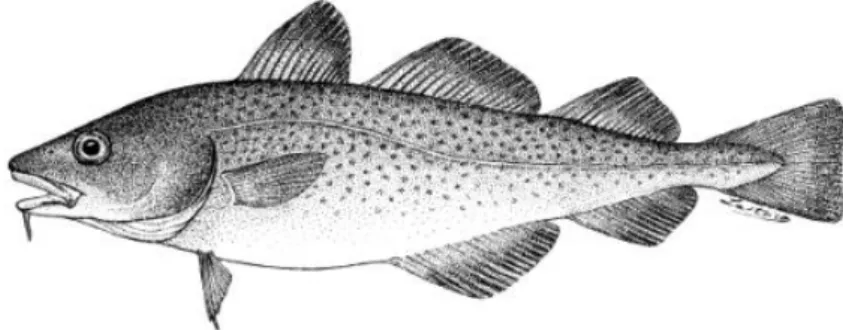
Figure 2. Gadus morhua, the Baltic’s top predator fish. Because of the strong decrease in the eastern Baltic population of cod researches focus on detecting the causes of its decline (Cohen 1990).
6
Otoliths (sagittae) (Fig. 4.), calcareous inner ear structures of fish, have been termed
“the black box” of fish because of the time-resolved information that they can provide about a fish’s life and biology (Degens et al. 1969, McMahon et al. 2011, Grønkjær et al. 2013). Otoliths are gradually formed over the life-time of a fish, by accruing calci- um carbonate around an organic protein matrix, otolin (Degens et al. 1969, Gauldie 1993, Grønkjær et al. 2013) as well as small amounts of different trace elements tak- en up from the environment (Kalish 1989, Marohn et al. 2011). The otolith is metabol- ically inactive i.e., once protein or organic material is settled down it cannot be further modified through metabolic processes (Rowell et al.
2010, Grønkjær et al. 2013). In the process, annual rings are added, which can be counted similarly to the age determination of trees (Campana 1999). Histori- cally, since roughly the year 1900, otoliths have been therefore collected by fisheries resource management institutes for the ageing of fish, and collections are available for many fish stocks around the world.
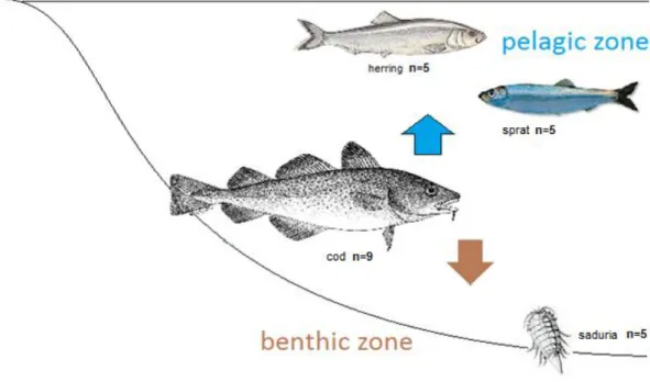
Figure 3. Schematic description of the cod’s feeding ecology: the blue arrow shows the cod’s pelagic food sources represented by herring and sprat, the brown arrow shows the cod’s benthic food sources represented by saduria. The numbers behind the organisms represent the number of organisms used in this study, f.e.” cod n=9” 9 cod individuals were used in this study.
Figure 4. Pair of otoliths (sagittae) of Gadus morhua.
Drawing of Jonas Mölle.
7 More recently otoliths attract
more applications: otoliths shape, microchemistry profiles and stable isotope values of inorganic otoliths material (aragonite) can be used as a natural tag of nursery (Dierking et al. 2012), migration patterns (Campana 1999, McMahon et al. 2011) and stock structure (Campana & Casselman 1993).
DNA from otolith surface can be used to reconstruct genetic time
series (Jakobsdottir et al. 2006) and address questions related to fisheries-induced evolution and population structure changes (Bonanomi et al. 2015). A novel applica- tion of otoliths has been developed even more recently, using the organic matrix of otoliths that presents roughly 0.2 to 10% of the otolith mass (Degens et al. 1969, Hüssy et al. 2004, Grønkjær et al. 2013). Pilot studies show the potential feasibility of using the organic component to reconstruct feeding ecology information, using stable isotope analysis (SIA) (McMahon et al. 2010, McMahon et al. 2011, Grønkjær et al.
2013). Those first approaches are big steps towards the application of otoliths to re- construct time series of fish diet, but still more investigation and development in un- derstanding of the results is needed.
Since the 1980s, stable isotope analysis (SIA) has become an essential ap- proach to understand ecosystem functioning (Peterson & Fry 1987) complementing traditionally used stomach content analysis (SCA) (Hyslop 1980). SIA measurements are based on the stable nature of heavy and light stable isotopes of elements, and due to the predictable fractionation from one trophic level to the next. With each next trophic level heavier isotopes accumulate in the animal’s tissue, therefore analysis of the isotopic depletion or enrichment of a tissue can reveal the trophic level (primary producer, consumer, top consumer) of the analysed individual, based on: “you are what you eat” (DeNiro & Epstein 1978, Fry 2006). 15N provides information about the trophic position.
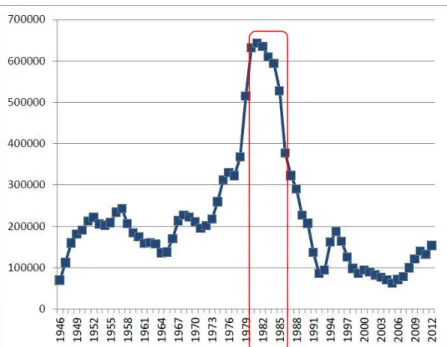
Figure 5. Graph of the decline of the eastern Baltic cod population after the regime shift in the 1980s (modified from (HELCOM 2013)).
8 On average, the pattern observed is: the higher is the trophic level, the more en- riched the 15N values, with top predators. 15N is an almost pure diet record, be- cause of the small fractionation from one trophic level to the next. 13C has been used for tracing pelagic (primary) producers and benthic organisms. Measurements of 34S are particularly powerful to distinguish between benthic and pelagic sources.
34S values are powerful tools for ecosystems like the Baltic Sea (Fig. 6.), where 13C is particularly limited because of its resolution. It shows some discrepancies in the distinction between different marine food sources (Peterson & Fry 1987, Fry 2006, Mittermayr et al. 2014, Mohm & Dierking *unpublished*).
There are two kinds of SIA, the bulk SIA i.e. the measurements of isotope ratio of tissues and the compound-specific stable isotope analysis, which measures the iso- tope value of certain components of tissues (Larsen et al. 2013, Larsen et al. 2015).
The bulk SIA is now one of the most influential tools in ecological studies, but the quantification of the relative importance of different food sources in the long-term diet of a species can be difficult in particular if many food sources are present or if tissue- specific fractionation factors are not well understood (DeNiro & Epstein 1981, McMahon et al. 2011).
Figure 6. Schematic plot of 13C and 15N isotope enrichment/depletion indicating the trophic level within a food chain in a marine ecosystem (Agurto 2007).
9 CSIA can overcome these obstacles. In the CSIA values of single components like, for example AAs, are measured, this leads to higher resolution that allows better dis- tinction between multiple food sources (McMahon et al. 2011, Larsen et al. 2013).
AAs, especially the essential AAs (EAAs), are much more independent of isotope baselines, whereas baselines of bulk SIA can vary strongly across different seasons and locations (McMahon et al. 2011, Larsen et al. 2013, Mohm & Dierking thesis 2014). Small fractionation factors (0 ‰ to 1 ‰) in essential AAs, and larger fractiona- tion in non-essential AAs have been shown in previous bone collagen and otolith studies (O'Brien et al. 2002, Jim et al. 2006, McMahon et al. 2010), underlining the importance of separation AAs and at the same time advantage of the EAAs. Both bulk SIA and CSIA traditionally focused on soft tissues, e.g., muscles, of organisms and addressed one or few time points, but not long-term data series. Therefore anal- ysis of organic material preserved out of hard structures such as bones or fish otoliths are a promising avenue to reconstruct the feeding ecology of organisms that lived and died a long time ago (DeNiro & Epstein 1978, 1981, Rowell et al. 2010, McMahon et al. 2011, Grønkjær et al. 2013, Wiley et al. 2013). A limiting factor for these analyses is the protein amount obtained from otoliths.
There is only a small proportion of protein in otoliths. The current method of the compound-specific analysis is not adjusted to such a small amount of material, so only cod of a defined size with big enough otoliths (otoliths mass > 150mg) can be analysed. Principle methods were addressed for wild fish and laboratory grown fish (Rowell et al. 2010, McMahon et al. 2011, Grønkjær et al. 2013) in order to estimate tissue-specific fractionation factors for otolith proteins bulk SIA using C and N, but never confirmed for S. A pilot data set on compound-specific stable isotope analysis (CSIA) for C was performed, comparing muscle CSIA and otolith CSIA, but not for the same individuals.
This study makes use of an existing cod otolith collection at GEOMAR, Helm- holtz-Zentrum für Ozeanforschung Kiel in the Department of Evolutionary Ecology of Marine Fishes conducted as a part of the Baltic Sea integrative long-term data series since 1996. The goals are (1) to confirm the feasibility of otolith protein bulk SIA (C, N, S) and assess CSIA on this tissue, for the first time for a commercially important fish, and also to compare these results with analyses of the traditionally used muscle tissue.
10 (2) To use cod otolith protein bulk SIA (C, N, S) and CSIA data and place it into a framework of isotopic signatures of potential diet sources to assess the feasibility of the reconstruction of a long-term feeding ecology data series on Baltic cod for a bet- ter understanding of ecological shifts over the past decades (Fig. 5.). Our goal is to create a tool set for using otoliths like “time machines”.
Material and Methods Study area
The Baltic Sea is a semi-enclosed brackish water area (Fig. 1. & 8.). It is character- ized by a vertical stratification on its water layers, and a long residence (turnover) time for full exchange of its water mass estimated at 25-30 years (Thulin &
Andrushaitis 2003). These features are major factors for the natural environmental conditions of the Baltic Sea: low salinity (between 1-20 psu with an average of 7 psu) eutrophication, oxygen-minimum and oxygen-hypoxia zones. In terms of global changes these conditions are getting more and more extreme, challenging the Baltic organisms even more (ICES 2008, Pachur & Horbowy 2013, BalticSTERN 2014,
Figure 7. Hypotheses of this study presented as questions. This thesis consists of two sub-parts: methodology and biology. For each part individual questions were designed.
11 Carstensen et al. 2014). Inflows of oxygen rich, saline and therefore heavier water from the North Sea and the large impact of river fresh water results in stratification of the water column in the whole Baltic.
The timing of the inflow events is un- predictable and infrequent, due to the climatic variability. These inflows are estimated to be very important for the productivity and a general well-being of the biota (Carstensen et al. 2014).
In this study we will focus on one of the deep basins of the Baltic - the Bornholm Basin, SD 25 (Thulin &
Andrushaitis 2003)(Fig. 8.). Bornholm Basin is very important for eastern Bal- tic cod recruitment (Fig. 1.) (Bagge et al.
1994, Tomkiewicz et al. 1998), and is the most important fishing ground in the Baltic Sea (Köster et al. 2003).
Study organism
The Baltic Cod (Fig. 2.) is a representative of the Gadidae family, presenting a brown to greenish color with a light lateral line and a conspicuous barbell on its lower jaw (Cohen et al. 1990). It can reach up to 115 cm in the Baltic Sea, but such big exam- ples are rare due to the high fishing pressure (Svedäng & Hornborg 2014). Cod plays a key role in Baltic ecosystem controlling the abundance of lower trophic levels via top-down control. Juvenile cod (<25 cm) have been described to prey on inverte- brates like Mysis species, Pontopoeira species and Bylgides sarsi, larger individuals (25-35 cm) on small clupeids (herring, sprat) and also benthic prey, especially Saduria entomon and larger fish (>35 cm) on pelagic organisms, clupeids like sprat (Sprattus sprattus) and herring (Clupea harengus L.) (Fig. 3.). Cannibalism also oc- curs and increases with the growth of the fish. Stomach content analysis has shown that benthic food sources are essential for cod diet (Bagge et al. 1994, Pachur &
Figure 8. Baltic Sea divided in subdivisions (SD), which is necessairy for management purposes. Fishes from SD 25 were examine in this study (ICES 2008).
12 Horbowy 2013, Mohm & Dierking *unpublished*). The role of cod in the food web has changed after species regime shift. It has been suggested that the benthic prey has become less available for cod, resulting in enhanced preying on pelagic clupeids, but significant evidence could not be done so far (Eero et al. 2015).
Sampling
The sampling of fish was carried out on the research cruise AL 435 on the vessel Alkor in April 2014. All fishes used in this study were sampled in Bornholm Basin, ICES SD 25 (Fig. 8.), captured by pelagic trawls (“Jungfischtrawl”, JFT) with a mesh size of 0.5 cm. We chose 12 cod individuals from 335 collected cod. Each cod was weighted (+/- 1g) and total length of the fish was measured, rounded to the next low- er cm. Moreover, sex (male, female, juvenile) and maturity stage of each individual was characterized.
We then dissected and dried the otolith pairs (sagittae) (Fig. 4.) and measured their length, width, and weight. We differed between left and right otoliths and label- ing each one differently.
From all these fishes muscle samples were taken carefully, without skin or blood, using a biopsy punch (4 mm; Stiefel; Durham,USA) or a scalpel. Samples were transferred into 2 ml polyethylene tubes (Sarstedt; Nümrecht, Germany), la- beled and frozen immediately at – 20°C to avoid degradation process.
Sampling design
To best cover potential ontogenetic shifts in feeding ecology, we divided the collected cod by size in 3 groups: small (35-39 cm), middle (40-45 cm) and big (50-55 cm) fishes, and chose 3 representatives from each group for the study.
To assess the applicability of different stable isotope analyses on otolith pro- tein we used two different approaches: bulk stable isotope analysis (bulk SIA) of car- bon (C), nitrogen (N) and sulfur (S), and compound specific stable isotope analysis (CSIA) of C, on two different sample types: otolith protein and muscle tissue, which is the tissue used the most in studies applying stable isotope analysis for fish. To an- swer our hypothesis, we used the following approach:
13 I: Left otoliths of the 9 specimen were used for the compound-specific isotope analy-
sis (13CAA).
II: Right otoliths, also 9 however, for bulk stable isotope (13C,NS).
III: 9 specimen for the muscle- tissue compound specific isotope analysis (13CAA) and 12 specimen for the muscle bulk stable isotope (13C,NS).
IV: Bulk stable isotope analysis (13C) of 3 different cod samples were used to compare left and right otoliths (Fig. 9.).
For both analyses, the bulk SIA and CSIA, we used the same specimen for a pair wise comparison. That will allow us a better evaluation of the feasibility of these 2 approaches and the best application for future studies.
Finally, to derive conclusions about cod feeding ecology from the bulk SIA and CSIA otolith protein results, with both methods (bulk SIA and CSIA) we created a framework by defining isotope values of benthic and pelagic prey (Fig. 3). The pelag- ic prey representatives used in the study were the clupeids: herring (Clupea harengus L.) (n=5) and sprat (Sprattus sprattus L.) (n=5), we studied also the benthic invertebrate prey Saduria entomon (n=5). From each prey we have chosen 5 repre-
Figure 9. Sampling design for the methodology part. In this study our goal is to test the possible use of otoltihs for retrocative - reconstructions of feeding ecology of fishes. For that purpose we performed 2 approches for defining food sources by using otoliths of fish, comparing those to the common used muscle-tissue with known patterns. Number “9” symbolised the number of analysed individuals. Dark line represents 2 comparision (“Bulk”= bulk SIA) within the methods itself. Comparing same individuals but different tissues, the red line represends the comparision of the the 2 approches.
14 sentatives for our analysis (Fig. 3.). In addition, a large framework of fish muscle tissue bulk SIA of C and N values was available from the same cruise from a parallel study on Baltic fish community feeding interactions (Mohm & Dierking *unpublished*).
Sample Preparation
Extraction the organic matrix out of otoliths
The analysis focuses on this organic matrix, the otolin. The extraction of the otolith protein is carried out in three steps, following Grønkjær at al.2013.
Cleaning of otoliths is necessary to make sure that the obtained protein is only from the otoltihs and not from the adhered tissue. We transferred the otoliths into glass tubes and covered with O.2M NaOH for at least 30 min. After sonification for 1- 2 min, we removed the rest of the adherent tissue by using a toothbrush. Finally, were washed those 3 times in Milli-Q water and dried out at 30°C for 48h. To improve the chemical process in the next step, the otoliths had to be grinded to a fine powder and transferred into 5ml microtubes.
Demineralization was used to remove the inorganic carbon from the otolith powder. We transferred 2 ml of 5°C 0.1 mol·L-1 HCL into the microtubes with otolith powder inside. We stored the otoliths first at 5°C to start the demineralization. Once the demineralization started we placed the microtubes at room temperature for 1-2h.
Afterwards we put the samples for 4-5 days into a heating cabinet to improve the demineralization process. Samples were then transferred into polyethylene test tubes.
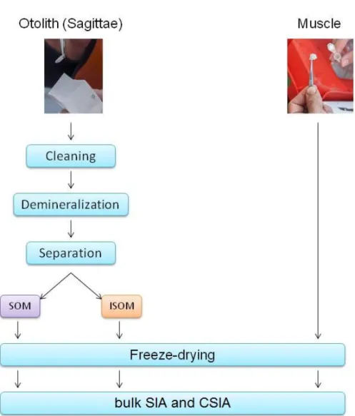
Separation of the bulk organic material, by centrifugation at 15 000 r·min-1 for 15min.The separation was improved by cleaning the test tubes with MilliQ water and centrifugation 3 times. The supernatant (SOM: soluble organic material) and the pre- cipitate (ISOM: insoluble organic material) separate visually. SOM was immediately transferred into cleaned Amicon Ultra filters. The HCL of the demineralization pro- cess was cleaned out from the SOM samples by adding 3.5 ml MilliQ water twice to the ultra filters centrifuged each time at 4000 r·min-1 for 2-3 min until the volume of the sample reached 50-100 µL. This volume we transferred into pre weighed poly- ethylene tubes.
15 The ISOM precipitate left in the microtubes was cleaned twice by adding 1ml MilliQ water each time into the tubes and centrifugation at 15 000 r·min-1 for 10 min.
ISOM pellet was transferred into pre weighed tin vial using 70µL MilliQ water. The separation of the bulk organic material was necessary only for the bulk stable isotope analysis. Both samples were freeze-dried.
All this was performed by Peter Grønkjær Department of Bioscience, Aarhus University, Ole Worms Alle 1, 8000 Aarhus C, Denmark.
Muscle samples
All muscle samples were freeze-dried (freeze-dryer alpha 1-1; Christ GmbH;
Osterode am Harz, Germany) and pulverized using a mortar and pestle. We then weighed 40-60 µg (MC 5 Micro Balance; Sartorius; Göttingen, Germany) of the pow- der into tin caps (3.2 x 4 mm) and added 25 mg ± 1 mg of Vanadium (V)-oxide.
We weighed 2.00 mg ± 0.10 mg of the muscle powder for CSIA into tin caps of 5 x 8 mm (Filter Scale SE2F; Sartorius; Göttingen, Germany). The muscle CSIA was per- formed in exactly the same way, like the otolith CISA. For bulk SIA we measured 40- 60 µg.
We used the same specimen for otolith proteins and muscles as well as for both of the analyses in order to provide comparable results (Fig. 9. & 10.). All the steps of sample preparation for both analyses are visualized in Fig. 10.
16 Stable isotope analysis (SIA)
Principle of bulk stable isotope analysis (bulk SIA)
All elements occur in multiple forms, termed as isotopes - it means elements that dif- fer in the number of neutrons, but have the same place in the periodic table (Fry 2006). In reactions different isotopes of one element behave slightly different, caused by isotope effects. An additional neutron does make the element more “heavier”, re- sulting in different discrimination in comparison to the lighter isotope (Farquhar et al.
1989, Mittermayr et al. 2014).
The method can be applied for migration studies in aquatic (Michener et al.
2007, Dierking et al. 2012) and terrestrial (DeNiro & Epstein 1978, 1981, van der Merwe & Medina 1991) ecosystems, analyses of movement and stock structure for fisheries (Campana & Thorrold 2001) and diet studies (Mittermayr et al. 2014, Mohm
& Dierking thesis 2014).
The fractionation factors () quantify isotope fractionation, it can be expressed by:
o-d = Ro / Rd,
For muscle tissue has been well investigated for many species: on average, the fractionation factor from one trophic level to the next is 0.5-1.5‰ for 13C (DeNiro &
Epstein 1978, Peterson & Fry 1987, Sweeting et al. 2007b) and roughly (=0.2‰) for S (Peterson & Fry 1987) (Fig. 6.). For fish the specific N muscle enrichment factor has been assessed by approx. 3.2‰ relative to prey (Sweeting et al. 2007a).
For cod juveniles enrichment factors for muscle (1.23‰ for 13C and 4.36‰ for N) (Ankjærø et al. 2012) and otolith proteins (SOM-fraction: 0.14‰ for 13C and 0.51‰
for N)(Grønkjær et al. 2013) where established.
Within an organism the isotope values can differ among different tissues. This phenomenon is called “routing” (Gannes et al. 1997). It can be caused by different turnover times of tissues or due different needs and the use tissue-specific nutrients by different tissue types. The consequence is that those tissues do not reflect exactly the same isotopic composition of the diet. In sum, in our measurements the resulting isotopic signature contains the mean isotopic value and the tissue specific fractiona- tion factor (Gannes et al. 1997).
17 This study is meant to contribute more knowledge towards the interpretation of the isotope values of otolith-proteins. Therefore, we will assess the very well established way of interpretation of muscle isotope values on our findings and compare those to our otolith-protein results of the same individuals in order to find a way for under- standing of the otolith-protein values.
For a correct estimation of the trophic position of the analysed organisms, it is necessary to analyse their potential prey. For this reason, we inserted cod’s isotopic signature into a frame work of its diet. Then we then were able to reconstruct food sources of cod.
Figure 10. Diagram of the different steps for sample preparation. Soluble organic material (SOM), insoluble organic material (ISOM) and muscles are freeze-dried and analyses for either bulk SIA or CSIA separatly.
18 Stable isotope analysis of samples
With bulk SIA we measured the extracted organic matrix of the right otolith and fish muscle tissue. The otolith protein consist two fractions: soluble (SOM) and insoluble material (ISOM), which we measured separately from each other, because of report- ed significant differences in isotope values of these different fractions (Grønkjær et al.
2013).
For the measurements we weighed 30-50 µg of ISOM, 100-300 µg of SOM and 40-60µg of the muscle tissue. Each sample was weighed into 3.2 x 4 mm tin caps adding 25 mg ± 1 mg of Vanadium (V)-oxide short before folding the tin caps.
Bulk SIA was carried out by continuous flow isotope ratio mass spectrometry (EA- IRMS/ GCC-IRMS) in the laboratory of Dr.Thomas Hansen at GEOMAR, Helmholtz- Zentrum für Ozeanforschung Kiel Experimentelle Ökologie I (Nahrungsnetze), Düsternbrooker Weg 20, 24105 Kiel
Samples were analysed and corrected for standards for 13C, 15N, 34S .Stable isotopes are expressed in delta values (13C, 15N, 34S).
X (‰) = [(Rsmpl /Rstnd)-1] * 1000‰,
where X is 13C ororS, R stand for the ration of heavy to light isotope an Rsmpl is the ratio of the sample and Rstnd the standard. Standard materials for reference were Vienna Pee Dee Belmnite (PDB) for carbon(C), atmospheric nitrogen (N2) and SO2
for sulfur (S).
Principle of compound-specific stable isotope analysis (CSIA for 13C AA)
We applied CSIA to gain information about the origins of food sources. We focused on essential amino acids (EAA) because consumers cannot synthesize them de novo and therefore depend on them from dietary sources. Metazoans can only synthesize about half of the 20 protein AAs. The EAA can only be synthesized by bacteria, fungi and plants. Organisms that do not synthesize them are obligated to obtain this with their diet.
Algae, bacteria, fungi and plants synthesize essential AA differently (Larsen et al. 2009). These differences in biosynthetic pathways and precursors result in source
19 characteristic 13C patterns among amino acids. Determining the 13C composition of those amino acids can therefore provide a distinct signal of the biosynthetic source.
This approach is called 13C fingerprinting of amino acids and proved to be a valua- ble tool for identifying food sources to consumers (Larsen et al. 2009, Larsen et al.
2013, Larsen et al. 2015)
Sample Preparation and Analysis for CSIA
For the CSIA in all samples we combined soluble and insoluble material, freeze-dried and homogenized them with a mortar. We weighted at least 2.00 mg ± 0.10 mg of the sample (muscle or otolith), to get a clear signal.
Samples were flushed with N2 gas, sealed and hydrolyzed in 1-2 ml 6 N HCl (37% HCl diluted with Milli-Q water, Merck, Darmstadt, Germany) at 110°C in a heat- ing block for 20h. After hydrolysis we removed lipophilic compounds by adding 2ml n- hexane/DCM (6:5, v/v) to the Pyrex tubes that were flushed shortly with N2 gas and sealed before vortexing for 30 s. The aqueous phase was then filtered through a Pasteur pipette lined with glass wool that had been pretreated at 450°C. All samples were transferred into the 4ml dram vials before evaporating the samples to dryness under a stream of N2 gas for 30min at 110°C in a heating block. The samples were stored at -18°C. To volatize the AAs, we followed the derivatization by Corr at al (Corr et al. 2007) methylating the dried samples with acidified methanol and subse- quently acetylating them with a mixture of acetic anhydride, triethylamine and ace- tone (NACME: N-acetyl methyl ester derivatives). To avoid oxidation of amino acids during derivatization, we flushed and sealed reaction vial with N2 gas. To account for carbon added during derivatization (Silfer et al. 1991) and variability of isotope frac- tionation during analysis, we also derivatized and analyzed pure amino acids with known δ13C values. Nor-leucine was used as an internal standard. Amino acid de- rivatives were injected with an autosampler into an Agilent Single Taper Ultra Inert Liner (#5190-2293) held at 280°C for 2 min.
The compounds were separated on a Thermo TraceGOLD TG-200MS GC column (60m x 0.32mm x 0.25um) installed on an Agilent 6890N gas chromatograph (GC). The oven temperature of the GC started at 50°C and heated at 15°C min-1 to 140°C, followed by 3°C min-1 to 152°C and held for 4 min, then 10°C min-1 to 245°C and held for 10 min, and finally 5°C min-1 to 290°C and held for 5 min. The GC was
20 interfaced with a MAT 253 isotope ratio mass spectrometer (IRMS) via a GC-III com- bustion (C) interface (Thermo-Finnigan Corporation). From each sample three repli- cates were made. All this was performed by Thomas Larsen and me in the Leibniz- Labor für Altersbestimmung und Isotopenforschung, Kiel.
Data are expressed in delta values as
X= (‰) [(Rsmpl /Rstnd)-1] * 1000‰,
where X is an amino acid, R stand for the ration of heavy to light isotope, where Rsmpl
is the ratio of the sample and Rstnd the standard.
We were able to analyze amino acids the following were defined as non-essential for animals: alanine (Ala), asparagine/aspartic acid (Asx), glutamine/glutamic acid (Glx), glycine (Gly), and tyrosine (Tyr). The following were defined as essential: histidine (His), isoleucine (Ile), leucine (Leu), lysine (Lys), methionine (Met), phenylalanine (Phe), threonine (Thr), and valine (Val). All amino acid values (13C) were corrected for the carbon added during derivatization (Larsen et al. 2013).
Data analysis
We used Excel 2007 (Microsoft Corporation; Redmond, USA) for evaluation of the data. MINITAB (Minitab Incorporated; State College, USA) we used for scatterplots, individual value plots, boxplots and statistical analysis, included paired t-tests, and ANOVAs. We considered the results as significant when p < 0.05. To visualize the output of the CSIA results, we performed principal component analysis (PCA) and linear discriminant analysis (LDA).
To assess differences in 13CAA patterns between tissue types we applied principal component analysis (PCA) with R version 3.2.2 using the vegan package.
PCA is a technique used to emphasize variation and bring out strong patterns in a dataset. PCA achieves this by eliminating uninformative parts. In addition to PCA we examine variables for the ones that visualize the differences for separation of groups the best way by performing LDA. LDA is been applied to emphasizes the differences of groups. We performed LDA with R version 3.2.2 using the MASS package and with MINITAB
21 0
100 200 300 400 500
10 30 50 70
otolith mass (mg)
fish length (cm)
I
0 100 200 300 400 500
5 10 15 20
otolith mass (mg)
otolith lenght (mm)
III
0 5 10 15 20
10 30 50 70
otolith length (mm)
fish length (cm)
II Results
Relationship of otolith length / weight and cod individual data
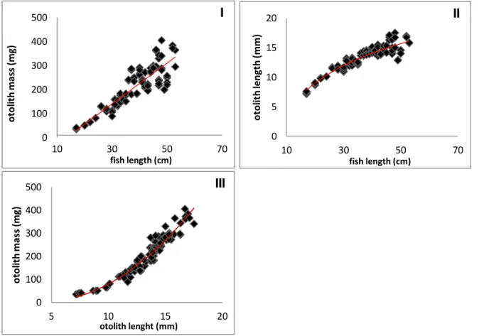
Otoliths grow over the life time of a fish by synthesizing a new growth ring every year, each of those consists of calcium carbonate and protein. To get a better understand- ing of the growth patterns of Baltic cod’s otoliths we studied the otoliths before the preparation for the stable isotope analyses. We measured the length, width and the mass of 12 otoliths and then compared the results with the morphometrics of the equivalent fish. The results show that otoliths grow linearly with the fish i.e., the big- ger the fish (TL), the heavier are its otoliths (Fig. 11.”I”). The Otoliths length growth is spatially limited, therefore it slows down at a certain size and mass increases (Fig.
11.”II”). The otolith’s volume increases cubically (a3) to the length of the fish (Fig.
11.”III”).
Figure 11. Reults of length, width and mass measurements of the cod otoliths. In figure ‘I’ the otoliths’ mass is plotted in relation to the fish length, the otolith’s mass increases proportionally to fish length. Figure ‘II’ shows the relation between otolith length and fish length.Otolith volume increases cubically to fish length. In figure ‘III’ the otolith mass is compared to the otolith length.
22 bulk SIA
Method applicability testing
How do bulk SIA values (C, N, S) differ between muscle tissue and otolith protein of the same cod individual?
In the analysis we compared within 3 groups: otolith-ISOM vs. otolith-SOM (13C: - 1.6‰ ± 0.4‰15N: 1.9‰ ± 0.3‰; 34S: 2.4‰ ± 0.8‰), muscle vs. otolith-ISOM (13C: 0.4‰ ± 0.3‰; 15N: 1.6‰ ± 0.3‰; 34S: 1.7‰ ± 0.6‰), and muscle vs. otolith- SOM (13C: -0.3‰ ± 0.3‰; 15N: 3.5‰ ± 0.3‰; 34S: 4.1‰ ± 0.8‰). We found signif- icant and consistent differences (paired ANOVA, holm–typ, :p< 0.05) for 15N and
34S isotopes in all groups. For 13C the only significant difference found was be- tween otolith-ISOM and otolith-SOM (Fig. 12, Table 1.).
Tissue 13
12 11 10 9
Otolith-SOM Otolith-ISOM
Muscle
-20.5 -21.0 -21.5 -22.0 -22.5
Otolith-SOM Otolith-ISOM
Muscle 18
16
14
6.0 5.5 5.0 4.5 4.0
d 15N d 13C
d 34S C/N
Figure 12. Comparison of 15N, 13C, 34S isotope values of the 3 different sample types visualised in boxplots. Results before the correction with the tissue-specific fractionation factor, we applied a paired ANOVA (holm-typ)test to verify the comparisons within the isotopes (15N, 13C , 34S) and the C/N-ratio.
23 We found that both fractions, ISOM and SOM, lock a comparable diet information like muscle tissue, because of the strong correlation (R > 0.7) that we estimated between individual isotope values of otolith protein and muscle. 13C values were almost iden- tical when comparing ISOM with muscle (R = 0.705, p-value = 0.01, R2 = 49.7) and SOM with muscle (R = 0.758, p-value = 0.004, R2 = 57.5). ISOM is also linearly cor- related to muscle for 15N with a relationship of R=0.751(p–value = 0.005, R2 = 56.5) (Fig. 13.).
Considering both, the consistency of the differences between the analysed sample types and the significant linear regression, we determined shifts (Table 2.).
These shifts are a specific difference between a certain otolith protein fraction (ISOM or SOM) and a muscle value. We used the shifts (Table 2.) to provide theoretical muscle values that were in turn used for interpretation in the biological part of this study.
ISOM vs.
SOM
Muscle vs.
ISOM
Muscle vs.
SOM
δ15N δ13C δ34S δ15N δ13C δ34S δ15N δ13C δ34S
P-Value *** *** *** *** *** *** ***
ISOM - SOM Muscle - ISOM Muscle - SOM
δ15N δ13C δ34S δ15N δ13C δ34S δ15N δ13C δ34S
Mean: 1.9 -0.6 2.4 1.6 0.4 1.7 3.5 -0.3 4.1
SD: 0.3 0.4 0.8 0.3 0.3 0.6 0.3 0.3 0.8
ISOM-muscle SOM-muscle ISOM-muscle SOM-muscle
15N R= 0.751 R= 0.603 R-sq= 56.5 R-sq=36.3
p-Value 0.005 0.038 0.005 0.038
13C R= 0.705 R= 0.758 R-sq=49.7 R-sq=57.5
p-Value 0.01 0.004 0.01 0.004
34S R= 0.627 R= -0.138 R-sq=39.3 R-sq=1.9
p-Value 0.029 0.668 0.029 0.668
Table 1. Comparison of 15N, 13C, 34S isotope values of the 3 different sample types visualised in a table. The statistical analysis (paired ANOVA) was applied to verify the comparisons. *** p<0,001, ** p<0,01, * p<0,05; red means not significantly different, green means the compared tissues are significantly different.
Table 2. Comparison of 15N, 13C, 34S isotope values of the 3 different sample types visualised in a table. Here we demonstrate the mean values with the standard deviation of the differences between the isotope values of the sample types.
Table 3. Summary of the linear relationship and regression values of 15N, 13C, 34S linearly discriminated for ISOM values vs. muscle values and SOM values vs. muscle values. The left column is the output of the linear relationship, the right column is the output of the regression. P-values were estimated for each linare relationship and regression analysis.
24 How strongly do bulk SIA values differ between otolith protein from left and right otoliths of the same fish?
First of all we compared the morphometrics and performed paired t-tests. We found that otoliths of different sides do not differ significantly in their length (p < 0.903) and weight (p < 0.809). In the literature we could not find any evidence for the similarity of the organic composition between right and left otoliths. To be sure about the similarity of both, we performed bulk SIA on right and left otolith proteins and estimated differ- ences (Table 3.). We compared both organic matrixes: SOM and ISOM values of right and left otoliths (Fig. 14. & 15.).We then analysed the output of bulk SIA with statistical analysis (paired t-test). The results also proved that right and left otoltihs are similar (p > 0.005) in their organic components (Table 4.).
Figure 13. Linear relationship of otolith protein and muscle stable isotope values of Baltic cod. Both otolith fractions, ISOM and SOM were compared with muscle values of the same specimen. Isotope values of 15N (first row)and13C (second row) were plotted. The broken red line represents the 1:1 line. Scales are the same only among the panels with the 13C values.
25
Figure 14. Individual value plots for a comparison between left and right otolith proteins for SOM isotope values (15N,
13C, 34S ) and for the C/N-ratio. We identified no significant difference neither within the isotopes nor the ratio.
Figure 15. Individual value plots comparing left and right otolith proteins for ISOM isotope values (15N, 13C, 34S ) and for the C/N-ratio. We identified no significant difference neither within the isotopes nor the ratio.
26 Biological case study
Cod in context of prey
We compared the bulk SIA values obtained for cod with values of its potential prey for each of the three analysed delta values (15N, 13C, and 34S). We first tested whether the application of the tissue-specific fractionation factor reported by Grønkjær et al. 2013 leads to comparable results between the cod otolith SOM frac- tions and the muscle values of cod (Fig.16.). Since we found no evidence for similari- ty between these sample types we performed an opportunistic way of interpretation of the bulk SIA. We used the previously estimated shifts to assess the theoretical muscle bulk SIA values for cod’s otolith proteins. The calculated theoretical SIA val- ues had comparable signals to the real muscle values of cod, and still differ accord- ing to the tissue characteristic variability. We then applied the fractionation factor for muscles (2-4‰) to our theoretical muscle bulk SIA values and interpreted the results considering the potential prey of cod.
Figure 17 and figure 20 show the array of the analysed organisms: the fourbeard rockling (Enchelyopus cimbrius L.) had the highest 15N value of 14.6 ‰, followed by whiting 13.5‰ (Merlangius merlangus L.). Both cod- muscle and the the- oretical muscle value presented a 15N mean of 13‰ (Fig. 22.), while flounder had 12.8‰. The invertebrate Saduria entomon showed a very similar isotope value like herring with approximately 11.7‰ of 15N for Saduria and 11.6 ‰ for herring. We observed the lowest 15N value for sprat with 10.5 ‰.
To distinguish between pelagic and benthic feeding fish, we analysed the iso- tope signatures of 13C and 34S.
ISOM SOM
δ15N δ13C δ34S δ15N δ13C δ34S
Mean difference 0.0 0.2 0.0 -0.2 0.0 0.1
SD 0.2 0.2 0.1 0.5 0.3 0.7
P-Value 1 0.456 1 0.506 0.84 0.83
Table 4. Summary of results of the paired t-test of bulk SIA values of right and left otolith proteins in order to estimate the similarity of left and right otolith proteins. Our results showed that right and left otolith proteins were not significantly different in their composition (p> 0.005).
27 We observed weak differences between pelagic and benthic organisms by using the
13C isotope values (Fig. 18) and very clear separation when using 34S (Fig. 19. &
20.).
According to the figure 18 we identified benthic representatives (the samples with a more enriched 13C): fourbeard rockling and cod, both with -21.3‰. According to these results the pelagic representatives would be: herring (-22.1‰), sprat (- 22.4‰) and saduria (-22.4‰). Saduria is a well known invertebrate, and it is clearly a benthic representative. Whiting (-21,9‰) and flounder (-22.0‰) were intermediate and therefore no allocation in pelagic or benthic feeding fish could be performed.
Thus bulk 13C analysis proved not to be applicable in our case.
Isotopic signatures of 34S have proved to be a better choice for distinguishing pelagic and benthic feeders (Fig. 19. & 20.). Here we assumed pelagic feeders to be:
herring (17.5‰) and sprat (17.1‰), as well as whiting (19.2‰) and cod (18.1‰).The benthic representatives were determined by their low 34S isotope values. According to this, benthic feeders were: fourbeard rockling (11.7‰), flounder (11.3‰) and saduria (12.4‰).
Tissue 10.0
9.5 9.0 8.5
Otolith-SOM Muscle
10.0 9.5 9.0 8.5
Otolith-SOM Muscle
-20.5 -21.0 -21.5 -22.0 -22.5
-20.5 -21.0 -21.5 -22.0 -22.5
d 15N-1 d 15N-2
d 13C-1 d 13C-2
Figure 16. Comparison of 15N, 13C, 34S isotope values of the 3 different sample types visualised in boxplots. Results after the correction with the tissue-specific fractionation factor. The applied t-test showed significant differences between the tissues.
28
d 15 N
9-whiting 8-flounder
7-fourbeard rockling 6-saduria
5-herring 4-sprat
3-cod-SOM 2-cod-ISOM
1-cod-M 15 14 13 12 11 10 9
Figure 17. Boxplot of 15N isotope value of all analysed Baltic-organisms: cod (muscle, otolith-ISOM, otolith-SOM), flounder, fourbeard rockling, herring, saduria, sprat and whiting).
d 13C
9-whiting 8-flounder
7-fourbeard rockling 6-saduria
5-herring 4-sprat
3-cod-SOM 2-cod-ISOM
1-cod-M -20.0 -20.5 -21.0 -21.5 -22.0 -22.5 -23.0 -23.5
Figure 18. Boxplot of 13C isotope value of all analysed Baltic-organisms: cod (muscle, otolith-ISOM, otolith-SOM), flounder, fourbeard rockling, herring, saduria, sprat and whiting).