Research Collection
Journal Article
Minimum transmissivity and optimal well spacing and flow rate for high-temperature aquifer thermal energy storage
Author(s):
Birdsell, Daniel T.; Adams, Benjamin M.; Saar, Martin O.
Publication Date:
2021-05
Permanent Link:
https://doi.org/10.3929/ethz-b-000473035
Originally published in:
Applied Energy 289, http://doi.org/10.1016/j.apenergy.2021.116658
Rights / License:
Creative Commons Attribution 4.0 International
This page was generated automatically upon download from the ETH Zurich Research Collection. For more information please consult the Terms of use.
ETH Library
Applied Energy 289 (2021) 116658
Available online 26 February 2021
0306-2619/© 2021 The Authors. Published by Elsevier Ltd. This is an open access article under the CC BY license (http://creativecommons.org/licenses/by/4.0/).
Contents lists available atScienceDirect
Applied Energy
journal homepage:www.elsevier.com/locate/apenergy
Minimum transmissivity and optimal well spacing and flow rate for high-temperature aquifer thermal energy storage
Daniel T. Birdsell
a,∗, Benjamin M. Adams
a, Martin O. Saar
a,baGeothermal Energy and Geofluids Group, Department of Earth Sciences, ETH Zürich, Sonneggstrasse 5, 8092 Zürich, Switzerland
bDepartment of Earth and Environmental Sciences, University of Minnesota, 116 Church Street SE, Minneapolis, MN, 55455, USA
A R T I C L E I N F O
Keywords:
High-temperature aquifer thermal energy storage
HT-ATES Heat storage Reservoir engineering Levelized cost of heat Geothermal energy
A B S T R A C T
Aquifer thermal energy storage (ATES) is a time-shifting thermal energy storage technology where waste heat is stored in an aquifer for weeks or months until it may be used at the surface. It can reduce carbon emissions and HVAC costs. Low-temperature (< 25◦C) aquifer thermal energy storage (LT-ATES) is already widely- deployed in central and northern Europe, and there is renewed interest in high-temperature (>50◦C) aquifer thermal energy storage (HT-ATES). However, it is unclear if LT-ATES guidelines for well spacing, reservoir depth, and transmissivity will apply to HT-ATES. We develop a thermo-hydro-mechanical-economic (THM$) analytical framework to balance three reservoir-engineering and economic constraints for an HT-ATES doublet connected to a district heating network. We find the optimal well spacing and flow rate are defined by the
‘‘reservoir constraints’’ at shallow depth and low permeability and are defined by the ‘‘economic constraints’’
at great depth and high permeability. We find the optimal well spacing is 1.8 times the thermal radius. We find that the levelized cost of heat is minimized at an intermediate depth. The minimum economically-viable transmissivity (MEVT) is the transmissivity below which HT-ATES is sure to be economically unattractive. We find the MEVT is relatively insensitive to depth, reservoir thickness, and faulting regime. Therefore, it can be approximated as5⋅10−13m3. The MEVT is useful for HT-ATES pre-assessment and can facilitate global estimates of HT-ATES potential.
1. Introduction
The heating and cooling of buildings comprise roughly half of the world’s final total energy consumption and are driven primarily by fossil fuels, resulting in substantial emissions of greenhouse gases [1], NOx, and SOx[2]. Thermal energy storage may reduce greenhouse gas emissions in two ways. First, in a system where heating and electricity networks are integrated, thermal energy storage can facilitate demand side management, which may lead to augmented use of variable re- newable electricity sources like wind and solar [3]. Second, seasonal thermal energy storage can shift the thermal energy supply to times of thermal energy demand [1], thereby potentially reducing the amount of energy required and carbon emitted. Seasonal thermal storage can be located in underground pits, tanks, mines, caverns, and aquifers, where large amounts of sensible heat can be stored with high efficiency.
Aquifer thermal energy storage (ATES) has the largest storage capacity among these options [1].
Typical ATES operations involve two stages: a summer stage and a winter stage. In the summer stage, water is extracted from a ‘‘cold’’
well, heated with waste heat that cannot be otherwise utilized, and
∗ Corresponding author.
E-mail address: danielbi@ethz.ch(D.T. Birdsell).
then re-injected into a ‘‘hot’’ well. In the winter stage, this process is reversed, and water is extracted from the hot well, used for heating, and is injected into the cold well at a lower temperature. As opposed to direct-use geothermal heating, ATES treats the reservoir as a storage tank and not an energy source. ATES’s heat is typically used in large commercial or industrial buildings, city-wide district heating networks (DHNs), or greenhouses.
There are two classes of aquifer thermal energy storage: low- temperature ATES and high-temperature ATES. Low-temperature ATES (LT-ATES) typically stores temperatures less than 25◦C. LT-ATES is widely implemented and generally considered technically and economi- cally successful, with thousands of installations worldwide and payback periods between 2–10 years [1]. In addition to heating, many LT-ATES systems are also used for cooling in the summer. This cooling is possible because the cold well has a sufficiently low temperature to accept heat. High-temperature ATES (HT-ATES) typically stores temperatures greater than 50◦C. In contrast to LT-ATES, HT-ATES is only used for heating because the temperature at the cold well is too high for cooling purposes [4].
https://doi.org/10.1016/j.apenergy.2021.116658
Received 3 November 2020; Received in revised form 10 February 2021; Accepted 11 February 2021
Nomenclature Acronyms
ATES Aquifer thermal energy storage COP Coefficient of performance
DHN District heating network
GETEM Geothermal electricity technology evalua- tion model
HF Hydraulic fracturing
HT-ATES High-temperature aquifer thermal energy storage
LCOH Levelized cost of heat
LT-ATES Low-temperature aquifer thermal energy storage
MEVP Minimum economically-viable permeability MEVT Minimum economically-viable transmissiv-
ity
NRGF Natural regional groundwater flow THM$ Thermo-hydro-mechanical-economic Superscripts and Subscripts
∗ Optimal value
𝑒𝑐𝑜𝑛 Related to the ‘‘economic constraints’’ and the ‘‘economic-constrained regime’’
𝐼,𝐼 𝐼,𝐼 𝐼 𝐼 Related to the first, second, and third constraint, respectively
𝑟𝑒𝑠 Related to the ‘‘reservoir constraints’’ and the ‘‘reservoir-constrained regime’’
𝑡ℎ Thermal
Variables and Parameters
𝛼𝐼 𝐼 Ratio of the minimum principal stress to the lithostatic stress
𝛼𝐼 Fraction of reservoir volume available for heat extraction
𝛥𝐿 Assumed distance for temperature gradient approximation
𝛥𝑃𝑖𝑛𝑗 Change in pressure at injection well 𝛥𝑇 Temperature difference between the ex-
tracted hot fluid and the injected cold fluid during the heat extraction stage
𝛥𝑡 The duration of heat extraction
𝜂 Thermal efficiency
𝛾 The ratio of HT-ATES’s heating cost to the cost of electricity
𝜆𝑒𝑓 𝑓 Effective thermal conductivity
𝜇 Dynamic fluid viscosity
𝜙 Porosity
𝜌𝑓 Fluid density
𝜌𝑟 Rock density
𝐴 Interfacial area for heat-loss calculation
𝑏 Reservoir thickness
𝑐 Price of electricity
𝐶1 Conversion constant [kWh/J]
𝐶𝑐𝑎𝑝 Capital cost
𝐶𝑜𝑝 Annual operating cost
𝐶𝑝,𝑓 Fluid heat capacity
𝐶𝑝,𝑟 Rock heat capacity
𝐶𝑅𝐹 Capital recovery factor
𝐷 Well diameter
𝑑 Reservoir depth
𝑑∗
𝑐𝑜𝑛𝑠𝑡𝑟𝑎𝑖𝑛𝑡𝑠 The depth where all three constraints are equal
𝑑∗
𝑘𝑚𝑖𝑛 The depth where the MEVP is minimized 𝑑𝐿𝐶𝑂𝐻∗ The depth where the LCOH is minimized 𝐸 Total amount of heat extracted during the
‘‘Heat Extraction’’ stage
𝑘 Permeability
𝐿 Well spacing
𝑚 Mass flow rate into injection well and out of production well
𝑛 Project lifetime
𝑄 Annual heat recovered
𝑄𝑐 Conductive heat loss from the reservoir
𝑟 Discount rate
𝑅𝑡ℎ Thermal radius
𝑇𝐶𝑉 Temperature in the heated control volume at the end of the resting stage
𝑇𝐷𝐻 District heat return temperature 𝑇𝐺 Background geothermal temperature 𝑇𝑊 𝐻 Summertime waste heat temperature 𝑉𝐻 𝐿 The reservoir volume from which heat is
lost
𝑉𝑟𝑒𝑠 Reservoir volume
𝑊 Work done by the pump during the extrac- tion stage
Previous studies recommend that well spacing should range from just over one [5] to more than three [6] thermal radii for LT-ATES.
The thermal radius is the radial extent of a thermal plume, assuming horizontal, cylindrical flow away from an injection well in a homo- geneous media [7]. Early work considered a doublet (i.e., a well pair) and showed that thermal breakthrough could significantly reduce the thermal efficiency [5]. More recently, work has considered LT- ATES planning at a city-wide scale, where many wells compete for limited subsurface space [7–9]. For cities with a congested subsurface, there is a tradeoff between optimizing an individual well’s thermal efficiency and maximizing the total amount of heat that can be stored underground by installing LT-ATES wells more densely. Therefore, it can make economic sense to reduce the well spacing somewhat to provide more heat [7,9]. In considering non-homogeneous reservoirs, Sommer et al. [10] found that heterogeneity in the permeability field increases the thermal diffusivity. Therefore, the optimal well spacing also depends on the degree of heterogeneity in the reservoir [10].
There are also recommendations on depth and transmissivity for LT-ATES. Reservoir transmissivity is the product of permeability and reservoir thickness. The permeability should be at least3⋅10−12 m2 and is more typically in the range of1⋅10−11–5⋅10−11m2[11,12]. The thickness should be at least 2 m and is more typically 20–50 m [11,12].
Therefore, the minimum transmissivity is on the order of 10−11 m3, with more typical values being one to two orders of magnitude higher.
The reservoir depth is typically 30–100 m, with an upper limit of 300 m [11]. Snijders and Drijver [11] suggest the upper limit on depth is due to economic feasibility.
HT-ATES has several potential advantages over LT-ATES. Firstly, higher temperature fluid has a higher energy density, and therefore each cubic meter has a higher economic value. Secondly, operating at higher temperatures could negate the need for a heat pump to upgrade the temperature before the fluid enters a DHN, thereby re- ducing complexity and capital costs [4]. Finally, HT-ATES can store large amounts of heat (up to 100 GW𝑡ℎh/yr [13]), and typically tar- gets deeper reservoirs than LT-ATES [4,13]. Therefore, HT-ATES could
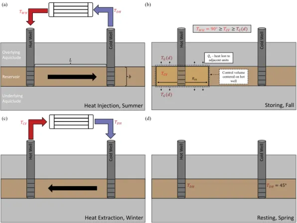
Fig. 1. Conceptual model of a HT-ATES doublet for (a) heat injection, (b) storing, (c) heat extraction, and (d) resting stages. Bold arrows indicate the direction of flow, when relevant.
potentially relieve the congestion due to LT-ATES in the shallow sub- surface under some cities by: (a) expanding the total thermal storage available and (b) targeting depths that do not compete with LT-ATES.
While the HT-ATES literature is more limited than the LT-ATES literature, it offers some insight into favorable permeability, reservoir thickness, and well spacing. Firstly, excessive permeability can result in significant advective heat loss due to thermally-driven buoyancy [14].
But on the other hand, if the permeability is too small, then it is difficult to inject and extract meaningful quantities of fluid and heat [15].
Therefore, it is likely that some intermediate permeability is favorable.
Secondly, the reservoir thickness affects the thermal efficiency by alter- ing the shape of the thermal stock and therefore the heat loss [15,16].
Finally, thermo-hydraulic numerical modeling with natural regional groundwater flow (NRGF) performed by Gao et al. [16] suggests that the well spacing should be 3.5 thermal radii.
Despite previous studies, guidelines for transmissivity, well spacing, and depth are not definitively established for HT-ATES. For one thing, there is no consensus on the suggested permeability and reservoir thickness. The value of permeability that is too large (i.e., associated with buoyancy-driven advective heat loss) is generally believed to be
≈ 5⋅10−13m2[14,17], but it could be one to two orders of magnitude higher [16]. The value of permeability that is too low (i.e., that limits fluid flow into and out of the reservoir) is also uncertain. It depends not only on thermal efficiency but also on avoiding hydro-mechanical problems that occur with excessive pore pressure [18] and on the levelized cost of heat (LCOH) that is deemed economically acceptable.
For reservoir thickness, the Résonance [15] study suggests that thin reservoirs are preferred, while the Gao et al. [16] study indicates that medium-thickness reservoirs are favorable. As a second point, most of the HT-ATES studies cited in the previous paragraph utilize parametric hydro-thermal numerical modeling. While this approach plays an important role in defining guidelines, it also has potential limitations. Firstly, it is hard to guarantee that guidelines taken from
these studies apply for all possible combinations of subsurface con- ditions. For example, the Gao et al. [16] recommendation for well spacing was found in the presence of NRGF, which encourages earlier thermal breakthrough than an initially-static reservoir. Secondly, while hydro-thermal models do an excellent job of constraining an HT-ATES system’s thermal efficiency, there are hydro-mechanical and economic aspects for which hydro-thermal models cannot provide insight.
In this paper, we model an HT-ATES doublet with varying reservoir transmissivity and depth. We find: (a) the flow rate, well spacing, and depth that is technically and economically attractive for HT-ATES sys- tems, and (b) the minimum economically-viable transmissivity (MEVT) of an HT-ATES reservoir, which is useful to pre-screen potential reser- voirs. In Section2, we develop a thermo-hydro-mechanical-economic (THM$) analytical framework to evaluate HT-ATES constraints related to reservoir engineering and economics. To our knowledge, this is a novel approach; previous studies have not coupled thermo-hydro- mechanical reservoir engineering and economics to create guidelines for HT-ATES. In Section3, we apply the THM$ framework to under- stand the optimal flow rate, well spacing, and depth. We also present LCOH calculations, which allow us to find the MEVT. Sections4and5 provide practical implications, discuss limitations of our approach, and conclude with main takeaways.
2. Methods
Our THM$ methodology considers a generic HT-ATES doublet, which is shown in Fig. 1 and discussed in more detail throughout Section2. The conceptual model includes four stages: (a) heat injection, (b) storing, (c) heat extraction, and (d) resting, which each last one quarter of a year and correspond roughly to summer, fall, winter, and spring, respectively. No water is injected or extracted through the wells in the storing or resting stages. Our THM$ framework can be expressed analytically, but it uses Python for variable passing, interpolation, and
to solve implicit equations. This code is published as an open-source companion to this manuscript [19].
Fig. 2shows a block-diagram overview of the THM$ calculations.
First, all the reservoir and economic parameters must be specified.
Second, the well spacing and flow rate are calculated in two ways: (a) from the reservoir constraints and (b) from the economic constraints (defined in Section2.3). Third, the optimal well spacing and flow rate are calculated as the minimum of the two well spacing and flow rate values, respectively. Finally, additional performance metrics such as the LCOH, thermal efficiency, heat loss, reservoir temperature, and MEVT are calculated.
While the summary of the THM$ methodology inFig. 2is simple, more detail must be provided in the following subsections. Sections2.1 and2.2provide governing equations for a well doublet and the three reservoir-engineering and economic constraints that the THM$ ap- proach considers. In Section2.3, we show how to calculate the optimal flow rate and well spacing. In Section2.4, we give more details about the equations used to describe heat loss and heat recovery, which are important to evaluate the economic attractiveness and other perfor- mance metrics of a HT-ATES system. In Section 2.5, we define the MEVT and explain the conservative assumptions behind it.
2.1. Overview equations for a well doublet
For a doublet system, the change in pressure at the injection well (i.e., the interface between the well screen and the porous media) is approximated by integrating the Darcy equation for fluid flow in porous media [20]:
𝛥𝑃𝑖𝑛𝑗= 𝑚𝜇 2𝜋𝜌𝑓(𝑘𝑏)ln
(𝐿 𝐷 )
(1) where 𝑚 is the mass flow rate into the injection well and out of the production well,𝜇 is the dynamic fluid viscosity,𝜌𝑓 is the fluid density, 𝑘 is the permeability, 𝑏is the reservoir thickness, 𝐿 is the well spacing, and 𝐷 is the well diameter. Eq. (1) assumes a flat, homogeneous, isotropic reservoir with a uniform initial hydraulic head, perfect aquicludes above and below, a fully-penetrating well, negligible changes in fluid density, and a system that has approached steady state. While simple, Schaetzle et al. [20] note that this solution gives relatively reliable results, and we confirmed in offline calculations that the error is typically less than 20% for the parameter ranges explored in this paper when compared to a more complex solution [21]. Since we are interested in a first-order, analytical analysis, we elect to use Eq. (1), due to its relatively simple form and relatively small error.
Note that 𝑘𝑏is the reservoir transmissivity with units of L3, and we keep these terms grouped in parenthesis throughout many equations in this paper to highlight the importance of transmissivity. The pressure change at the production well has the same magnitude but the opposite sign, so the total pressure difference between the two wells is2𝛥𝑃𝑖𝑛𝑗. By using Eq. (1), we are neglecting pressure losses very near the well (i.e., the skin factor) and within the wells. This is a reasonable approximation, since these tend to be smaller than pressure losses within the reservoir [22].
The COP is a measure of the useful heat extracted from the reservoir to the pumping work required to store and extract that heat. Dur- ing the heat extraction stage, the total amount of heat extracted is:
𝐸 = 𝑚𝐶𝑝,𝑓𝛥𝑇 𝛥𝑡 where𝐶𝑝,𝑓 is the water’s heat capacity,𝛥𝑇 is the temperature difference between the extracted hot fluid and the injected cold fluid during the heat extraction stage, and𝛥𝑡is the duration of the heat extraction. Assuming perfectly-efficient pumps, the work during the extraction stage is: 𝑊 = 2𝑚𝛥𝑃𝑖𝑛𝑗𝛥𝑡∕𝜌𝑓. Therefore, using Eq.(1), the COP during heat extraction can be expressed as:
𝐶𝑂𝑃 = 𝐸
𝑊 = 𝑚𝐶𝑝,𝑓𝛥𝑇 𝛥𝑡 2𝑚𝛥𝑃𝑖𝑛𝑗𝛥𝑡∕𝜌𝑓 =
𝜌2
𝑓𝐶𝑝,𝑓𝛥𝑇 𝜋(𝑘𝑏)
𝑚𝜇ln(𝐿∕𝐷) (2)
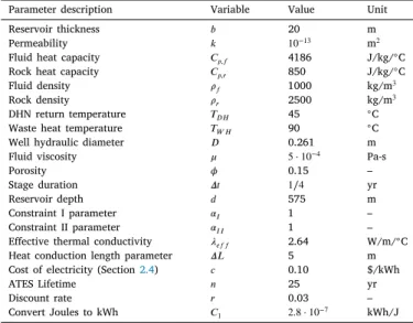
The parameters for our base-case scenario are shown inTable 1. If parameters are changed in parts of the Results (Section 3), they are explicitly noted.
Fig. 2.Block diagram for the THM$ calculations.
Table 1
Parameters for base-case scenario.
Parameter description Variable Value Unit
Reservoir thickness 𝑏 20 m
Permeability 𝑘 10−13 m2
Fluid heat capacity 𝐶𝑝,𝑓 4186 J/kg/◦C
Rock heat capacity 𝐶𝑝,𝑟 850 J/kg/◦C
Fluid density 𝜌𝑓 1000 kg/m3
Rock density 𝜌𝑟 2500 kg/m3
DHN return temperature 𝑇𝐷𝐻 45 ◦C
Waste heat temperature 𝑇𝑊 𝐻 90 ◦C
Well hydraulic diameter 𝐷 0.261 m
Fluid viscosity 𝜇 5⋅10−4 Pa-s
Porosity 𝜙 0.15 –
Stage duration 𝛥𝑡 1∕4 yr
Reservoir depth 𝑑 575 m
Constraint I parameter 𝛼𝐼 1 –
Constraint II parameter 𝛼𝐼 𝐼 1 –
Effective thermal conductivity 𝜆𝑒𝑓 𝑓 2.64 W/m/◦C
Heat conduction length parameter 𝛥𝐿 5 m
Cost of electricity (Section2.4) 𝑐 0.10 $/kWh
ATES Lifetime 𝑛 25 yr
Discount rate 𝑟 0.03 –
Convert Joules to kWh 𝐶1 2.8⋅10−7 kWh/J
2.2. Three constraints
In this paper, we analyze and balance three constraints that apply to HT-ATES systems:
• Constraint I defines a maximum flow rate so that the reservoir’s thermal capacity is not over-utilized.
• Constraint II defines a maximum flow rate so that the reservoir pressure does not lead to hydraulic fracturing (HF).
• Constraint III defines the flow rate that minimizes the levelized cost of heat (LCOH). It does not make sense to pump at flow rates above the flow rate that minimizes LCOH, so Constraint III defines a ‘‘maximum’’ flow rate in the same way as Constraints I and II.
Constraint I is related to hydro-thermal reservoir engineering, Con- straint II is related to hydro-mechanical reservoir engineering, and Constraint III is related to economics (and hydro-thermal reservoir engi- neering to a lesser degree). These three constraints form the backbone of our THM$ approach. This is not a fully-coupled approach, which would require numerical simulation. Instead, we take an analytical approach which reduces complexity so that it is possible to consider insights from the full set of THM$ constraints with short computational times.
Constraint I defines the maximum flow rate for which a reservoir will be able to store heat effectively. The amount of heat that a reservoir
can hold is:(𝜌𝑓𝐶𝑝,𝑓𝜙+𝜌𝑟𝐶𝑝,𝑟(1 −𝜙))𝑉𝑟𝑒𝑠(𝑇𝑊 𝐻−𝑇𝐷𝐻), where𝜙is the porosity, 𝜌𝑟 is the rock density, 𝐶𝑝,𝑟 is the rock’s heat capacity, 𝑉𝑟𝑒𝑠 is the useful reservoir volume, and 𝑇𝑊 𝐻 −𝑇𝐷𝐻 is the temperature difference between the injected and extracted fluid during the heat injection stage (seeFig. 1and Section2.4for more detail). We assume that the useful reservoir volume is 𝑉𝑟𝑒𝑠 = (𝛼𝐼𝐿)2𝑏, where𝛼𝐼 is the fraction of the reservoir volume available for heat extraction and has an assumed value of one. The amount of energy injected during the heat injection stage is𝑚𝐶𝑝,𝑤𝛥𝑡(𝑇𝑊 𝐻−𝑇𝐷𝐻). By equating the amount of heat a reservoir can hold with the amount injected, we find a maximum flow rate, which is a function of, among other parameters, the reservoir thickness and well spacing:
𝑚𝐼≤(𝜙𝜌𝑓𝐶𝑝,𝑓+ (1 −𝜙)𝜌𝑟𝐶𝑝,𝑟)((𝛼𝐼𝐿)2𝑏)
𝐶𝑝,𝑓𝛥𝑡 (3)
If the flow rate exceeds𝑚𝐼, additional heat will not be stored effec- tively, and pumping electricity is wasted.
Constraint II defines the maximum flow rate that can be supported without HF the reservoir. HF occurs when the pore pressure exceeds the minimum principal stress plus the tensile strength of the rock. We neglect tensile strength and assume a form for the minimum principal stress as:𝛼𝐼 𝐼𝜌𝑟𝑔𝑑where𝛼𝐼 𝐼is the ratio of the minimum principal stress to the lithostatic stress and𝑑is the reservoir depth. For reverse faulting regimes, 𝛼𝐼 𝐼 = 1 according to Anderson’s faulting classifications, because the minimum principal stress is the lithostatic stress [23]. Our base-case scenario uses𝛼𝐼 𝐼= 1, which allows higher flow rates than if 𝛼𝐼 𝐼 <1, in normal and strike-slip faulting regimes. Assuming that the reservoir pore pressure is hydrostatic initially, and utilizing Eq.(1), we write the mass flow rate to avoid hydraulic fracturing.
𝑚𝐼 𝐼≤ 2𝜋𝜌𝑓(𝑘𝑏) 𝜇ln(𝐿∕𝐷)
(
(𝛼𝐼 𝐼𝜌𝑟−𝜌𝑓)𝑔𝑑 )
(4) By combining Eq.(2)with Eq.(4), we can also express Constraint II in terms of COP.
𝐶𝑂𝑃𝐼 𝐼 ≥ 𝜌𝑓𝐶𝑝,𝑓𝛥𝑇
2(𝛼𝐼 𝐼𝜌𝑟−𝜌𝑓)𝑔𝑑 (5)
Constraint III defines the flow rate that minimizes the LCOH. We calculate LCOH according to:
𝐿𝐶𝑂𝐻=𝐶𝑐𝑎𝑝⋅𝐶𝑅𝐹+𝐶𝑜𝑝
𝑄 = 𝐶𝑐𝑎𝑝⋅𝐶𝑅𝐹
𝑚𝐶𝑝,𝑓𝛥𝑇 𝛥𝑡𝐶1 + 2𝑚𝑐𝜇ln(𝐿∕𝐷) 𝜋𝜌2
𝑓(𝑘𝑏)𝐶𝑝,𝑓𝛥𝑇 (6) where 𝐶𝑐𝑎𝑝 is the capital cost, 𝐶𝑅𝐹 is the capital recovery factor, 𝐶𝑜𝑝 is the annual operating cost, and𝑄is the annual heat recovered.
The operating cost is the pumping work multiplied by the cost of electricity. Using Eqs. (1) and (2), it can be expressed as: 𝐶𝑜𝑝 = 2𝑚2𝛥𝑡𝐶1𝑐𝜇ln(𝐿∕𝐷)∕𝜋𝜌2𝑓(𝑘𝑏), where𝐶1= 2.8⋅10−7kWh/J is a constant to convert units, and 𝑐 is the price of electricity. The annual heat recovered in kWh is:𝑄=𝑚𝐶𝑝,𝑓𝛥𝑇 𝛥𝑡𝐶1. Maintenance costs are assumed to be negligible. The capital costs occur at the beginning of the project and are assumed to be twice the cost of the wells, which agrees with costs for the ATES system in Rostock, Germany [12]. The well cost is taken from the Geothermal Electricity Technology Evaluation Model (GETEM) for a borehole with a 31 cm diameter and is expressed in terms of 2019 US dollars [24]. Multiplication of capital cost with the capital recovery factor turns the capital cost into an equivalent annualized cost.𝐶𝑅𝐹 is defined as:
𝐶𝑅𝐹 = 𝑟(1 +𝑟)𝑛
(1 +𝑟)𝑛− 1 (7)
where𝑟is the discount rate and 𝑛is the lifetime of the project. We assume a discount rate of 3%, a twenty-five year project lifetime, and an electricity cost of $0.10/kWh.
The flow rate that results in the minimum LCOH can be found by taking the derivative of Eq.(6)with respect to𝑚and setting to zero.
𝑑(𝐿𝐶𝑂𝐻)
𝑑 𝑚 = −𝐶𝑐𝑎𝑝⋅𝐶𝑅𝐹 𝑚𝑄 +𝐶𝑜𝑝
𝑚𝑄
= −𝐶𝑐𝑎𝑝⋅𝐶𝑅𝐹
𝑚2𝐶𝑝,𝑓𝛥𝑇 𝛥𝑡𝐶1 + 2𝑐𝜇ln(𝐿∕𝐷) 𝐶𝑝,𝑓𝛥𝑇 𝜌2
𝑓𝜋(𝑘𝑏)= 0
(8)
Solving the previous equation for𝑚gives the flow rate that minimizes LCOH:
𝑚𝐼 𝐼 𝐼=
(𝐶𝑐𝑎𝑝⋅𝐶𝑅𝐹 𝜌2
𝑓𝜋(𝑘𝑏) 2𝐶1𝑐𝛥𝑡𝜇ln(𝐿∕𝐷)
)1∕2
(9) If the flow rate is greater than the equation above, then the pumping cost is large, which increases the LCOH. If the flow rate is less than the equation above, then the LCOH can be decreased by increasing the flow rate, thereby recovering more heat each year. Interestingly, it can be seen from Eq.(8)that the LCOH is minimized when the annual operating cost equals the equivalent annualized capital cost.
2.3. Optimal flow rate and well spacing
The three constraints from the previous section can be further combined into the ‘‘reservoir constraints’’ and the ‘‘economic con- straints’’. The reservoir constraints include Constraints I and II. They apply at shallow depth or low permeability, and we call this part of the parameter space the ‘‘reservoir-constrained regime’’. The economic constraints include Constraints I and III. They apply at great depth or high permeability, and we call this part of the parameter space the
‘‘economic-constrained regime’’.
The optimal well spacing and flow rate have different relationships, depending if the HT-ATES reservoir exists in the reservoir-constrained regime or the economic-constrained regime.
• Reservoir-constrained regime:In the reservoir-constrained regime, the well spacing and flow rate are denoted𝐿𝑟𝑒𝑠and𝑚𝑟𝑒𝑠, respec- tively.𝑚𝑟𝑒𝑠represents the maximum flow rate that the reservoir can support, without HF or injecting more heat than the reservoir can hold. By equating𝑚𝐼 (Eq.(3)) with𝑚𝐼 𝐼 (Eq.(4)), we find an implicit expression for the well spacing:
(𝐿𝑟𝑒𝑠)2⋅ln(𝐿𝑟𝑒𝑠∕𝐷) −2𝜋𝜌𝑓𝑘 𝜇
(
(𝛼𝐼 𝐼𝜌𝑟−𝜌𝑓)𝑔𝑑 )
×
𝐶𝑝,𝑤𝛥𝑡
(𝜙𝜌𝑓𝐶𝑝,𝑓+ (1 −𝜙)𝜌𝑟𝐶𝑝,𝑟)= 0
(10)
• Economic-constrained regime:In the economic-constrained regime, the well spacing and flow rate are denoted 𝐿𝑒𝑐𝑜𝑛 and 𝑚𝑒𝑐𝑜𝑛, respectively. By equating𝑚𝐼(Eq.(3)) with𝑚𝐼 𝐼 𝐼(Eq.(9)), we find an implicit expression for𝐿𝑒𝑐𝑜𝑛:
(𝐶𝑐𝑎𝑝⋅𝐶𝑅𝐹 𝜌2
𝑓𝜋(𝑘𝑏) 2𝐶1𝑐𝛥𝑡𝜇ln(𝐿𝑒𝑐𝑜𝑛∕𝐷)
)1∕2
−(𝜙𝜌𝑓𝐶𝑝,𝑓+ (1 −𝜙)𝜌𝑟𝐶𝑝,𝑟)((𝛼𝐼𝐿𝑒𝑐𝑜𝑛)2𝑏)
𝐶𝑝,𝑓𝛥𝑡 = 0
(11)
The optimal well spacing and flow rate can be determined in several steps. First, the well spacing from the reservoir and economic con- straints (𝐿𝑟𝑒𝑠and𝐿𝑒𝑐𝑜𝑛, respectively) are calculated using Eqs.(10)and (11). Then, the flow rates from the reservoir and economic constraints (𝑚𝑟𝑒𝑠and𝑚𝑒𝑐𝑜𝑛) are calculated by using𝐿𝑟𝑒𝑠and𝐿𝑒𝑐𝑜𝑛, respectively, in Eq.(3). Finally, the optimal flow rate is set as the minimum of𝑚𝑟𝑒𝑠and 𝑚𝑒𝑐𝑜𝑛, which ensures that the three constraints from Section2.2are not violated. Similarly, the optimal well spacing is also set to the minimum of𝐿𝑟𝑒𝑠and𝐿𝑒𝑐𝑜𝑛.
2.4. Heat loss and recovery
As the depth and geothermal temperature increase, we expect less heat loss, greater thermal efficiency, and more overall heat produc- tion, if all else is held constant. This section develops a conceptual and mathematical model of heat loss and recovery that honors these aforementioned trends. Our conceptual model was introduced at the beginning of Section2and is illustrated inFig. 1, but we describe it in more detail here. During the heat injection stage, fluid is injected
into the hot well at the temperature supplied from the summertime waste heat source, 𝑇𝑊 𝐻. Simultaneously, fluid is produced from the cold well at a temperature of𝑇𝐷𝐻, the wintertime district heat return temperature. During the storing stage, we assume that heat is irrecover- ably lost from the reservoir to the aquicludes. We assume this heat loss occurs from a cylindrically-shaped control volume with thermal radius 𝑅𝑡ℎand thickness𝑏, and we define the average temperature at the end of the storing stage in the control volume as 𝑇𝐶𝑉. During the heat extraction stage, the remaining thermal energy in the control volume is recovered (to a cut off temperature of𝑇𝐷𝐻), such that𝛥𝑇=𝑇𝐶𝑉−𝑇𝐷𝐻 in Eqs. (2),(5), and (6). For simplicity, we assume that the DHN is perfectly efficient, so that all the heat at𝑇 > 𝑇𝐷𝐻 is useful to the DHN.
We do not consider the use of heat pumps, which could bring lower- temperature fluid up to a useful temperature for the DHN. In the resting stage, we assume that the water near the hot and cold wells remains at 𝑇𝐷𝐻, which is important for the start of the next heat injection stage.
We approximate the thermal efficiency of the HT-ATES system as:
𝜂= 𝑚𝐶𝑝,𝑓𝛥𝑡(𝑇𝐶𝑉−𝑇𝐷𝐻)
𝑚𝐶𝑝,𝑓𝛥𝑡(𝑇𝑊 𝐻−𝑇𝐷𝐻)= (𝑇𝐶𝑉−𝑇𝐷𝐻)
(𝑇𝑊 𝐻−𝑇𝐷𝐻) (12)
In Eq. (12), 𝑇𝐷𝐻 = 45 ◦C and 𝑇𝑊 𝐻 = 90 ◦C are assumed from surface constraints, which seem reasonable for HT-ATES and fourth- generation DHNs [25,26]. To solve for𝑇𝐶𝑉, we assume that heat losses are purely conductive to the overlying and underlying aquicludes.
Neglecting buoyancy-driven advective heat loss appears to be justified for𝑘 <5⋅10−13m2[14,17]. We assume that heat losses can be described by:
𝑄𝑐= −𝜆𝑒𝑓 𝑓𝐴∇𝑇≈ −𝜆𝑒𝑓 𝑓𝐴𝑇𝐶𝑉(𝑡) −𝑇𝐺
𝛥𝐿 (13)
where 𝜆𝑒𝑓 𝑓 is the effective thermal conductivity of the rock/water mixture,𝐴is the interfacial area between the hot control volume and the overlying and underlying rock, 𝑇𝐶𝑉(𝑡)is the temperature in the control volume as a function of time (and is distinct from𝑇𝐶𝑉 which is the temperature at the end of the resting stage),𝑇𝐺is the background geothermal temperature, and 𝛥𝐿is an assumed distance over which the temperature gradient is approximated. The geothermal temperature is a function of depth and assumes a surface temperature of 10 ◦C and a geothermal gradient of 30◦C/km. 𝛥𝐿is assumed to be 5 m, because previous modeling work has shown that the temperature fronts remain fairly sharp [14]. The use of𝛥𝐿 = 5m is further justified because it results in thermal efficiencies that are within the range of numerical models of HT-ATES for similar reservoir properties and cut- off temperatures [14,15]. By accounting for the energy accumulation and heat-loss terms, we can write an ODE for𝑇𝐶𝑉 and solve for the average temperature within the control volume as a function of time.
At the end of the resting stage, the temperature is:
𝑇𝐶𝑉 = (𝑇𝑊 𝐻−𝑇𝐺) exp (−𝐶3𝛥𝑡
𝐶2 )
+𝑇𝐺 (14)
where𝐶2 = ((1 −𝜙)𝜌𝑟𝐶𝑝,𝑟+𝜙𝜌𝑓𝐶𝑝,𝑓)𝑉𝐻 𝐿,𝐶3=𝜆𝑒𝑓 𝑓𝐴∕𝛥𝐿, and𝑉𝐻 𝐿is the reservoir volume over which heat loss occurs. Note that we used the initial condition𝑇𝐶𝑉(𝑡= 0) =𝑇𝐷𝐻 to arrive at the solution above.
The reservoir volume over which heat loss occurs can be approximated from either the well spacing or the thermal radius as𝑉𝐻 𝐿= (𝛼𝐼 𝐼𝐿)2𝑏 or𝑉𝐻 𝐿 =𝜋𝑅2
𝑡ℎ𝑏, respectively. Similarly, the interfacial area between the thermally-affected reservoir and the cold, overlying and underlying units can also be expressed in terms of the well spacing or the thermal radius as𝐴= 2𝐿2 or𝐴= 2𝜋𝑅2𝑡ℎ, respectively. It is not clear in general if the well-spacing or the thermal-radius provide better approximations of the heat loss volume and interfacial area. However, the thermal radius approximation does have one advantage: it scales the size of the thermally-effected region with the flow rate, and we therefore use 𝑉𝐻 𝐿=𝜋𝑅2
𝑡ℎ𝑏and𝐴= 2𝜋𝑅2𝑡ℎ.
2.5. Minimum economically-viable transmissivity
Our goal is to find the minimum economically-viable transmissivity (MEVT) (and a related measure, the minimum economically-viable permeability (MEVP)), which is the transmissivity (and permeability) below which HT-ATES is sure to be economically unattractive. The MEVT can provide a useful lower bound on reservoir transmissivity, allowing one to quickly and easily eliminate potential reservoirs that have a transmissivity below the MEVT. We take two steps to ensure that the MEVT truly is a lower bound on economic viability, so that reser- voirs are not unduly eliminated from consideration. Firstly, we define the MEVT as the transmissivity that results in HT-ATES LCOH being equal to the cost of an expensive heating alternative, namely electrical resistant heating. If we had chosen a cheaper heating alternative (e.g., a natural gas boiler), then the transmissivity would need to be larger to have cost parity. Secondly, we make many conservative assumptions in our HT-ATES model that favor lower LCOH. These assumptions include:
1. We neglect costs related to the construction and maintenance of a DHN, which are necessary for most large-scale HT-ATES.
2. We also neglect the maintenance costs of the HT-ATES system (see Section2.2).
3. Many of our reservoir-engineering assumptions promote high thermal recovery. For one example, we neglect advective heat loss, which promotes high thermal efficiency (Section2.4). Fur- thermore, we assume a reverse faulting regime for the base case (i.e., 𝛼𝐼 𝐼 = 1), which allows for higher flow rates than would be allowed in normal or strike-slip faulting regimes (see Section2.2). Finally, we assume a homogeneous reservoir, but heterogeneity would decrease the thermal efficiency [10,15].
We define𝛾as the ratio of HT-ATES’s LCOH to the cost of electricity.
Since the MEVT is defined with respect to the cost of electrical resis- tance heating, the MEVT is the transmissivity that results in𝛾 =1:1.
While the cost of electricity is an assumed value, it is less important than the ratio given by𝛾because the cost of electricity scales both the operating cost of HT-ATES and the cost of electrical resistance heating.
3. Results
In Section3.1, we plot the three constraints in terms of COP and flow rate, so that they can be compared visually. In Section3.2, we present results for the optimal flow rate and well spacing. In Sec- tion3.3, we explore the thermal performance as a function of depth.
In Section 3.4, we show the LCOH, the MEVP, and the MEVT. In Section3.5, we discuss the optimal depth for HT-ATES. Note that we use the optimal flow rate and well spacing throughout Section3, unless otherwise noted. When results are presented as a function of depth, the depth ranges from 50 m to 2667 m. We choose 2667 m as a cutoff because the geothermal temperature equals the waste heat temperature at this depth.
3.1. The three constraints
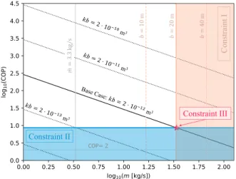
All three constraints are illustrated with respect to COP and mass flow rate inFig. 3. The black curves show COP versus mass flow rate from Eq.(2), with reservoir transmissivity indicated on the plot. The solid black line represents the base case, while the dotted lines have different values of permeability. Higher flow rates imply lower COP because the pumps must perform more work. Constraint I is illustrated by a family of yellow curves, which indicate different reservoir thick- ness values. Constraint I must be plotted as multiple curves because the reservoir volume depends on the reservoir thickness (Eq. (3)).
Constraint II is illustrated by a blue line (Eq.(5)), and Constraint III is represented by a red star for the base case. Note that the base case is a unique scenario chosen so that all three constraints imply the same flow rate. Under these circumstances, the flow rate and well spacing
Fig. 3. The logarithm of coefficient of performance (COP) plotted versus the logarithm of mass flow rate with three constraints overlaid. The black curves represent COP versus flow rate. The family of yellow curves represent Constraint I, the blue curve represents Constraint II, and the red star indicates the flow rate that minimizes LCOH from Constraint III (base case). The flow rate and COP must exist outside of the shaded regions from Constraints I and II and to the left of the flow rate implied by Constraint III. Other conditions that are unfavorable, such as COP<2 or low flow rate (arbitrarily chosen as<3.3 kg/s) are illustrated in gray. The well spacing is 151 m (which is optimal for the base case), and the depth is 575 m.
from the reservoir constraints are equal to those from the economic constraints. Still, if the reservoir depth, thickness, or permeability were changed, then only two constraints would overlap at the same flow rate.
The COP that leads to HF is independent of the flow rate (which we can see because the blue line is horizontal inFig. 3), permeability, and reservoir thickness (as indicated by inspection of Eq.(5)). Instead, it depends only on parameters related to the effective stress and the temperature difference. Practically speaking, an engineer can only change the depth or the temperature difference to alter the COP that leads to HF. Inspection of Constraint II highlights that the flow rate that leads to HF may be very low for some reservoir transmissivities.
To achieve a flow rate above3.3 kg∕swithout HF, the transmissivity must be greater than 2⋅10−13 m2 for the base-case depth and stress state. At greater depths, the overburden stress suppresses HF, and the flow rate can be larger, while at shallower depths, the flow rate would need to be less.
The COP=2 line indicates that the electric work put into pumping is equal to the thermal heat retrieved (i.e., it is equivalent to𝛾 =1:1 if capital costs are neglected). It is therefore interesting that Constraint II implies a COP that is much larger than 2, which holds for a broad range of parameters in Eq. (5). The COP associated with Constraint II indicates that an HT-ATES will recover more heat than the work that was put into pumping if HF does not occur. Furthermore, even though COP is a measure of thermal recovery efficiency with respect to pumping work, it should not be used to make decisions about the flow rate for HT-ATES. In fact, to maximize the COP, one would select a flow rate approaching zero, which would return essentially no heat. Metrics other than the COP, such as the LCOH (as discussed in Section3.4), may be more appropriate to make decisions about flow rate. Nevertheless, COP provides a valuable first step to eliminate sites with insufficient permeability.
3.2. Optimal well spacing and flow rate
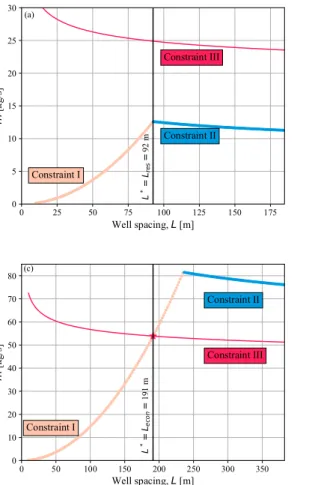
Fig. 4plots the flow rate versus the well spacing for each constraint.
Constraint I shows that as the well spacing increases, the flow rate in- creases because a larger reservoir volume can store more heat (Eq.(3)).
Constraint II shows that as the well spacing decreases, the flow rate can be increased without leading to HF (Eq.(4)). The maximum flow
rate that a reservoir can support (i.e.,𝑚𝑟𝑒𝑠) is found at the intersection between Constraints I and II. Under these conditions, all the heat is effectively stored, and HF does not occur. Note that in the reservoir- constrained regime, the flow rate is more sensitive to well spacing when 𝐿 < 𝐿∗than when𝐿 > 𝐿∗. Constraint III shows that the flow rate that minimizes LCOH increases as well spacing decreases (Eq.(9)). If the curves from Constraints I and III intersect, the well spacing and flow rate come from the economic constraints and should be operated at values lower than the maximum that reservoir can support (i.e.,𝐿∗= 𝐿𝑒𝑐𝑜𝑛≤𝐿𝑟𝑒𝑠and𝑚∗=𝑚𝑒𝑐𝑜𝑛≤𝑚𝑟𝑒𝑠).Fig. 4(a) shows a shallow reservoir in the reservoir-constrained regime. The flow rate is limited to13 kg∕s.
The LCOH could hypothetically be decreased with higher flow rates, as shown from the Constraint III curve, but this would lead to HF of the reservoir and therefore cannot be pursued.Fig. 4(b) is the base case.
Since it is a special case, all three constraints imply the same flow rate (33 kg/s) and well spacing (151 m).Fig. 4(c), shows a deeper reservoir that operates in the economic-constrained regime at𝑚∗=𝑚𝑒𝑐𝑜𝑛= 54 kg/s and𝐿∗=𝐿𝑒𝑐𝑜𝑛= 191m.
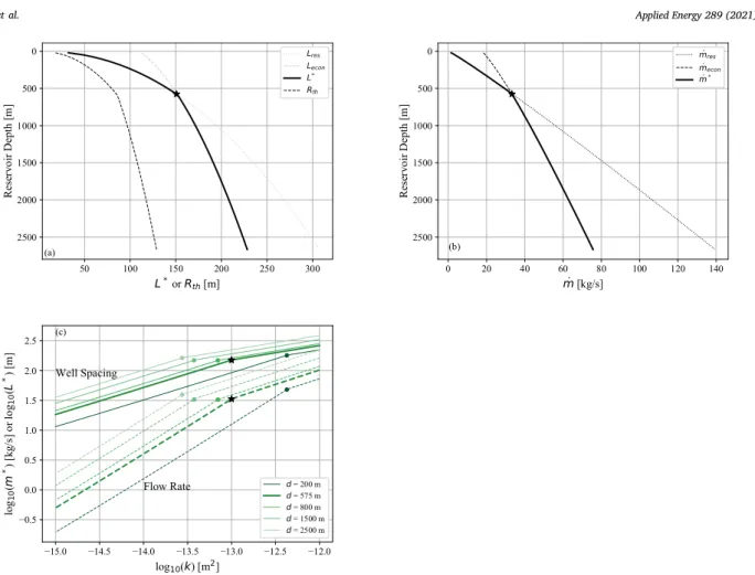
Optimal well spacing and flow rate increase monotonically with respect to depth, as shown in Figs. 5(a) and (b). The reservoir con- straints are relevant at shallow depth, while the economic constraints are relevant at great depth. In the reservoir-constrained regime, the op- timal well spacing and flow rate increase rapidly with respect to depth (although the well spacing increases at a decreasing rate). Physically, this is because a greater depth has a greater associated lithostatic stress, which allows both the flow rate and well spacing to increase without leading to HF (Constraint II), while storing all of the injected heat (Constraint I). In the economic-constrained regime, the well spacing and flow rate increase more slowly with respect to depth. Physically, this makes sense because the well spacing and flow rate are both limited below their maximum reservoir-constrained values (i.e.,𝐿𝑒𝑐𝑜𝑛<
𝐿𝑟𝑒𝑠 and𝑚𝑒𝑐𝑜𝑛 < 𝑚𝑟𝑒𝑠) within the economic-constrained regime. The economic constraints can lead to reductions of up to 64 kg/s and 79 m in the flow rate and well spacing, respectively, compared to the maximum flow rate the reservoir could support at a depth of 2667 m.
These reductions are equivalent to 46% for the flow rate and a 25% for the well spacing. The optimal well spacing is always1.8𝑅𝑡ℎ, regardless of depth.
The optimal well spacing and flow rate also increase monotonically with respect to permeability, as shown in Fig. 5(c). The reservoir constraints are relevant at low permeability, while the economic con- straints are relevant at high permeability. For the base-case depth, the transition point from the reservoir-constrained regime to the economic- constrained regime occurs near a permeability of 10−13m2. This transi- tion point occurs at smaller permeability as the depth increases, which matches physical intuition, because a smaller permeability leads to a larger pressure at the injection well (Eq. (1)), if the flow is held constant. Therefore, the transition happens at a greater depth, where larger lithostatic stress suppresses HF.
It is possible to draw conclusions directly from examining the equations in Section2. In the reservoir-constrained regime, Eq.(10) shows that the optimal well spacing is independent of the reservoir thickness. Examination of Eqs.(3)and(4)allows us to conclude that the flow rate is directly proportional to the reservoir thickness, in the reservoir-constrained regime. In contrast, in the economic-constrained regime, the well spacing depends on the reservoir thickness, as can be seen in Eq.(11). This dependence leads to a nonlinearity in the flow rate with respect to the reservoir thickness, since the flow rate depends on both the reservoir thickness and the well spacing (see Eqs.(3)and (9)), and the well spacing also depends on the reservoir thickness.
3.3. Thermal performance as a function of depth
The annual amount of heat injected, recovered, and lost to the surrounding rock is shown as a function of depth inFig. 6(a).
Fig. 4. Plots of mass flow rate versus well spacing to depict the constraints leading to optimal well spacing and flow rate at depths of (a) 200 m, (b) 575 m (base case), and (c) 1500 m. In (a), Constraints I and II (the reservoir-engineering constraints) limit the flow rate and well spacing. In (b), all three constraints are balanced and point to the same flow rate and well spacing. In (c), Constraints I and III (the economic constraints) limit the well spacing and flow rate. The red star shows the point where Constraints I and III intersect, when relevant.
The injected heat is proportional to the optimal flow rate in Fig. 5(b). The injected heat increases rapidly and linearly with respect to depth within the reservoir-constrained regime. This increase con- tinues at a slower (but still linear) rate in the reservoir-constrained regime.
The heat loss displays a non-monotonic relationship with respect to depth, but the thermal efficiency increases monotonically. The heat loss shows non-monotonicity due to trade-offs between: (a) the interfacial area for heat loss (i.e.,𝐴in Eq.(13)) and (b) the temperature gradient (which is proportional to𝑇𝐶𝑉 −𝑇𝐺in Eq. (13)). Going from shallow to deep, the heat loss initially increases due to the larger interfacial area. At 850 m deep, the heat loss hits its maximum. Below that depth, the temperature gradient, and therefore the heat loss per area, is small. Therefore, the heat loss decreases with depth, despite more heat injection and larger interfacial area. Even though the heat lost has a non-monotonic relationship with depth, the fraction of heat lost to heat injected decreases monotonically with depth. This trend results in increased thermal efficiency with depth, as shown inFig. 6(b). The results are presented down to depths of 2667 m, where the geothermal temperature equals the waste-heat temperature, heat losses become zero, and the thermal efficiency is100%. Trends about heat loss and thermal efficiency can be further understood by examining Eqs. (12) and(13)and examining𝑇𝑊 𝐻,𝑇𝐶𝑉,𝑇𝐺, and𝑇𝐷𝐻inFig. 6(b).
The heat recovered increases with respect to depth, due to the larger amount of heat injected and the higher thermal efficiency. This increase is approximately linear with respect to depth, with a large slope in the reservoir-constrained regime and a somewhat smaller slope within the economic-constrained regime. For our base case, 13.8 GW𝑡ℎh are injected, and 10.8 GW𝑡ℎh are recovered each year.
3.4. Levelized cost of heat and minimum economically-viable transmissivity
The LCOH is plotted as a function of depth inFig. 7(a). LCOH is large at shallow depths, hits a minimum at an intermediate depth, and gradually increases at greater depths. For the base-case scenario, LCOH varies by a factor of less than 2.5 with respect to depth, in the range of depths considered. The minimum LCOH is $0.040/kW𝑡ℎh at 272 m and increases up to>$0.08/kW𝑡ℎh for depths equal to 50 m and 2667 m.
Likewise, the LCOH is fairly insensitive to the faulting regime. The minimum LCOH for𝑏= 20m and𝛼𝐼 𝐼 = 0.8is $0.048/kW𝑡ℎh, which is approximately 20% larger than the base case with𝛼𝐼 𝐼= 1.0.
The LCOH minimum occurs because of a trade-off between the increased thermal performance with depth (as discussed in Section3.3) and the increased costs with depth. This trade-off is illustrated in Fig. 7(b), which shows equivalent annualized capital cost, annual op- erating cost, and annual heat recovered. The operating cost is insignif- icant at shallow depths, but the capital cost is high compared to the heat recovered. As depth increases, LCOH is minimized because the heat recovered becomes large compared to the capital cost, and the operating costs remain small. We denote the depth where LCOH is minimized as𝑑∗
𝐿𝐶𝑂𝐻. Since𝑑∗
𝐿𝐶𝑂𝐻 is a function of reservoir thickness and faulting regime, we discuss it in further detail in Section3.5. As depth continues to increase, operating cost increases at an increasing rate, which increases the LCOH. Going even deeper (in the economic- constrained regime), the operating cost is equal to the annualized capital cost (see Eq.(8)), and these combined costs are high enough that the LCOH continues to increase, despite recovering more heat as depth increases.
Fig. 5. Optimal well spacing and flow rate. In (a), the depth versus the optimal well spacing and thermal radius are shown. In (b), the depth versus the optimal flow rate is shown. In both (a) and (b), the dashed line indicates the value from the economic constraints, the dotted line indicates the value from the reservoir constraints, and the solid bold line indicates the optimal value, which overlaps the dotted or dashed line, depending on the regime. In (c), the well spacing (solid lines) and flow rate (dashed lines) are plotted versus permeability at different depths. The transition from the reservoir-constrained regime to the economic-constrained regime is marked with a black star for the base case in all three figures; the transition is marked with dots for other depths in (c).
Fig. 6. (a) Annual heat injected, recovered, and lost as a function of depth for a HT-ATES doublet. (b) Thermal efficiency (𝜂), control volume temperature at the end of the storing stage (𝑇𝐶𝑉), and geothermal temperature (𝑇𝐺) as a function of depth. Also shown in gray are the district heating return temperature (𝑇𝐷𝐻) and the waste heat supply temperature (𝑇𝑊 𝐻).
Fig. 8(a) shows the LCOH as a function of permeability for various reservoir thicknesses and faulting regimes (controlled by𝛼𝐼 𝐼). As per- meability decreases, the LCOH increases. At some critical permeability, the LCOH is equal to the cost of electricity. This is the MEVP, 𝑘𝑚𝑖𝑛, as was introduced in Section2.5. If the permeability falls below𝑘𝑚𝑖𝑛, heat could certainly be generated with electrical resistance heating for a lower cost than the HT-ATES could provide. The MEVP is marked with a star in Fig. 8(a) and is𝑘𝑚𝑖𝑛 = 2.8⋅10−14 m2 for the base-case scenario.
The MEVP depends on the depth, as shown inFig. 8(b). The MEVP is minimized at a depth of 465 m for the base case. We denote the depth where the MEVP is minimized as𝑑∗
𝑘𝑚𝑖𝑛, note that it is a function of reservoir thickness and faulting regime, and discuss in more detail in Section3.5.
While the MEVP is the permeability that results in a one-to-one ratio of heat to electric cost (i.e.,𝛾 =1:1), the analysis can be extended to look for the permeability that would result in lower LCOH and more favorable cost ratios.Fig. 9(a) plots the permeability as a function of
Fig. 7. (a) Depth versus LCOH and (b) depth versus annual operating costs (𝐶𝑜𝑝), equivalent annualized capital costs (𝐶𝑐𝑎𝑝⋅𝐶𝑅𝐹) and annual heat recovery per doublet (𝑄), for base-case permeability and reservoir thickness. In (a), the base-case scenario is plotted with a bold line, solid lines use𝛼𝐼 𝐼= 1, dotted lines use𝛼𝐼 𝐼= 0.8to represent an alternative faulting regime, and color shade corresponds to the reservoir thickness. In (b), various measures of optimal depth are also plotted for reference (see Section3.5).
Fig. 8. (a) The logarithm of LCOH as a function of the logarithm of permeability and (b) the reservoir depth versus the logarithm of the MEVP. The bold lines are used to indicate the base-case reservoir thickness, and the MEVP for the base-case reservoir thickness is marked by a star. The solid lines use the base-case faulting regime (i.e.,𝛼𝐼 𝐼= 1), dotted lines use the alternative faulting regime (i.e.,𝛼𝐼 𝐼= 0.8), and color shade corresponds to aquifer thickness (i.e.,𝑏).
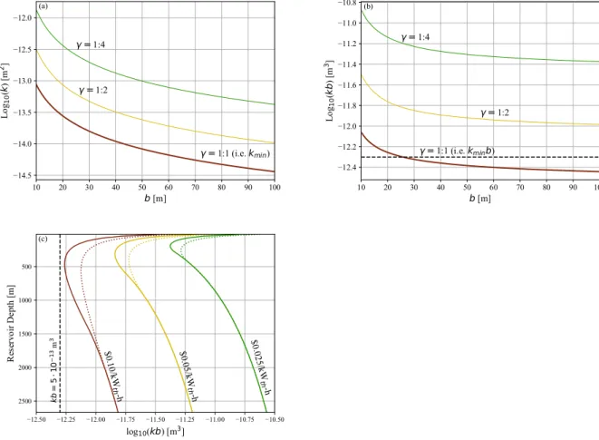
reservoir thickness that results in𝛾equal to 1:1, 1:2, and 1:4. The 1:2 and 1:4 ratios correspond to LCOH of $0.05/kWh𝑡ℎand $0.025/kWh𝑡ℎ, respectively. The permeability required for𝛾=1:4 is greater than ten times the permeability required for𝛾=1:1.
The MEVP decreases as the reservoir thickness increases, suggesting that the transmissivity may be a more important parameter than the permeability. The MEVT is the product of the MEVP and the reser- voir thickness, 𝑘𝑚𝑖𝑛𝑏, and is plotted versus the reservoir thickness in Fig. 9(b). Over the range of10< 𝑏 < 100m, the MEVP varies by a factor of 24, while the MEVT varies by only a factor of 2.4.
Fig. 9(c) shows contours of LCOH as a function of reservoir depth, transmissivity, and faulting regime. The LCOH is most sensitive to the transmissivity, with higher transmissivity associated with lower LCOH.
The LCOH is halved and quartered, respectively, by an increase in transmissivity by a factor of three and 12. The LCOH is less sensitive to depth and is minimized at an intermediate depth. For example, at 𝑘𝑏= 10−12.25m3, the optimal depth is at≈ 500m. Finally, the LCOH is relatively insensitive to the faulting regime, especially at great depths within the economic-constrained regime. This insensitivity is especially true at great depths (i.e., within the economic-constrained regime), where the solid and dashed lines overlap inFig. 9(c).
The red curve inFig. 9(c) depicts the MEVT. Like the other contours, it is relatively insensitive to depth and faulting regime. The MEVT varies by less than a factor of three with respect to depth over the range of 50 to 2667 m. Furthermore, the MEVT varies by less than a factor of 1.5 between𝛼𝐼 𝐼 = 1.0and 0.8.
3.5. Measures of optimal depth
In this section, we explore the optimal depth for an HT-ATES reservoir, which has two measures (introduced in Section3.4): (a) the depth where the LCOH is minimized,𝑑∗
𝐿𝐶𝑂𝐻, and (b) the depth where the MEVP is minimized,𝑑∗
𝑘𝑚𝑖𝑛. These optimal depth values are plotted in Fig. 10, and they range from 189 m to 742 m for the tested parameters (i.e., combinations of𝑏= 10, 20, and 40 m and𝛼𝐼 𝐼 = 1.0and 0.8). By both measures, the optimal depth becomes shallower as the reservoir becomes thicker. The optimal depth in the alternate faulting regime is deeper than the base-case faulting regime, due to the influence the stress state has on the HF pressure. We also plot the depth where all three constraints are equal,𝑑𝑐𝑜𝑛𝑠𝑡𝑟𝑎𝑖𝑛𝑡𝑠, which indicates where the reservoir-constrained regime transitions to the economic-constrained regime. The depth where LCOH is minimized is shallower than the depth where all three constraints are equal for all the combinations of parameters that we considered, and it is possible that LCOH is always minimized in the reservoir-constrained regime, although we did not exhaustively explore the parameter space.
4. Discussion
4.1. Optimal well spacing and flow rate
The optimal well spacing and flow rate are determined from either the reservoir constraints or the economic constraints, and choosing the correct well spacing and flow rate is essential both technically and