The hydrogen Molecular Ion Revisited
Jean-Philippe GRIVET
Copyright (2002) Journal of Chemical Education. This article may be downloaded for personal use only.
The following article appeared in J. Chem. Ed. 79, 127-132 (2002) and may be found at (URL/link for published article abstract)
The hydrogen molecular ion (HMI), the simplest mo- lecular system, was studied in the early days of quantum mechanics. The demonstration that this species had, in agree- ment with experiment, a stable ground state corresponding to a bond between two atoms, was one of the early achievements of quantum theory. Classical mechanics could not predict a stable state for H2+.
The molecular orbital method, in the form of a linear combination of atomic orbitals (LCAO-MO method), was proposed at that time; its first application was to the HMI.
Many other approximate treatments were then devised and applied to H2+ (see e.g. ref 1).
Burrau (2) showed that the confocal elliptic coordinate system allowed the complete separation of the HMI Hamil- tonian, thus paving the way toward an exact solution. This task was taken up by several investigators, including Burrau himself, Teller (3), Jaffé (4), and Hylleraas (5). They showed that the energy of any state of the HMI could be found by solving two coupled differential equations. Various methods of solution were proposed, all involving rather complicated expansions in series of associated Legendre functions. These led in turn to three term recurrence relations, from which intricate eigenvalue equations followed. In practice the ener- gies could only be found numerically; formulas to compute the expansion coefficients were also given. More recently, electronic computers have replaced humans and the energy of the HMI can be obtained in this formalism to at least seven significant figures (6–9).
The analytical solution of the HMI problem is mentioned in most textbooks dealing with molecular structure, usually with few details. Notable exceptions are Pauling and Wilson (1), Slater (10), and Levine (11). The present-day student can only get a glimpse of the method used, unless he or she chooses to read the original literature, at the risk of being
drowned in a morass of complicated algebra. Further, in con- trast to the LCAO–MO method, the analytical approach can hardly be generalized to other species. These facts explain why it is usually given short shrift in textbooks. Yet with the advent of powerful and inexpensive microcomputers, it should be possible for a student to repeat some of these com- putations and gain some feeling for the behavior of the HMI quantum system. It is the purpose of the present report to show that this goal is effectively within reach. We show here how the Schrödinger equation may be solved, keeping the required mathematics as simple as possible and letting the computer do most of the work. A similar point of view is taken by Press et al. (12). As we shall see, we will be able to obtain at once very accurate values of the wave function and of the energy and, in the process, learn how conserved quan- tities and quantum numbers are handled for a problem with cylindrical or D∞h symmetry.
This report should be of interest to advanced under- graduates in physical chemistry; it could be used as a start- ing point for a computational chemistry project. It may also be of historical interest to a wider audience.
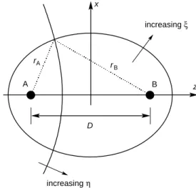
The Molecular Hamiltonian in Spheroidal Coordinates The Schrödinger equation describing the motion of an electron in the field of two infinitely massive protons HA and HB located at points A and B, a distance D apart on the z axis (Fig. 1) is, in Slater’s notation,
∇ 2– 2rA– 2rB ψr =Eψr (1) where rA and rB are the distances from the electron to the two protons. Following Slater, we use a system of atomic units in which the unit of energy is the rydberg or 13.6 eV; the unit of length is the radius of the first Bohr orbit, 0.529 Å.
It is necessary to introduce prolate confocal elliptic coordi- nates, ξ = (rA + rB)/D, η = (rA – rB)/D, and ϕ, which is the angle of rotation about the nuclear axis. The inverse relations are rA = D(ξ + η)/2 and rB = D(ξ – η)/2; we note that 2/rA= 4/[D(ξ + η)], 2/rB = 4/[D(ξ – η)]. The meaning of these defi- nitions becomes clear when we examine elliptic coordinates in a plane. The lines of constant ξ are ellipses, which share foci A and B. The lines of constant η are hyperbolas, again with A and B as foci. These two families form an orthogonal system of curves (see Fig. 1). The variable ξ plays a role analo- gous to r, the distance to the origin, in the usual polar coordi- nate system. When η increases, the point (ξ,η) moves around the origin, so that this parameter is similar to the quantity cosθ in polar coordinates. The domains of each variable are 1≤ η ≤ 1 and 1 ≤ ξ ≤ ∞. On the part of the z axis that lies between A and B, rA + rB = D, so that ξ = 1, while D ≤ rA – rB ≤ D, and 1 ≤ η ≤ 1. To the right of B (z ≥ 1 ), η = 1;
and η = 1 to the left of A (z ≤ 1 ).
The Hydrogen Molecular Ion Revisited
Jean-Philippe Grivet
Centre de Biophysique Moléculaire, C.N.R.S., and Département de Physique, Université d’Orléans, rue Charles-Sadron, 45071 Orléans cedex 02, France; grivet@cnrs-orleans.fr
Figure 1. Definition of planar confocal elliptic coordinates x
increasing ξ
rB rA
A B z
D
increasing η
Prolate ellipsoidal coordinates in space are obtained by rotating the figure around the z axis. The ellipses generate a set of confocal ellipsoids, while the hyperbolas generate a family of hyperboloids with two sheets. Surface of constant ϕ are half-planes though the x axis.
The derivation of the Laplacian operator in elliptic co- ordinates is found in several texts (10, 13, 14) and will not be repeated here. The volume element in spheroidal coordi- nates turns out to be
dV =D3
8 ξ2–η2 dξdηdϕ (2) The Laplacian is
∇2= 4
D2 ξ2–η2
∂ξ ξ∂ 2– 1 ∂ξ∂ +∂η∂ 1 –η2 ∂
∂η + 1
ξ2– 1+ 1 1 –η2 ∂2
∂ϕ2
(3)Using the relation r1A+ 1rB= 4
D ξ ξ2–η2
Schrödinger’s equation now reads, after some simple re- arrangements
∂ξ ξ∂ 2– 1 ∂ψ
∂ξ + ∂
∂η 1 –η2 ∂ψ
∂η + ξ21– 1+ 1
1 –η2 ∂2ψ
∂ϕ2+ c2 ξ2–η2 + 2Dξ ψ= 0 (4)
with
c2= 1
4E D2 (5)
According to the separation of variables method, we seek a solution of the form ψ = R(ξ)S(η)eimϕ. By analogy with the atomic case, we have assumed an explicit form of the ϕ de- pendence and introduced a so-called separation constant, m.
Inserting in eq 4, putting ∂2ψ/∂ϕ2 = m2ψ, and dividing throughout by the product RSeimϕ, we find that the various terms can be grouped in ξ- and η- dependent parts:
1
R ξ2– 1 R′ ′– m2
ξ2– 1+ 2Dξ+c2ξ2 + 1
S 1 –η2S′ ′– m2
1 –η2–c2η2 = 0 (6)
In order for this equation to hold for any value of ξ and η, the expressions within the two braces must be constant and of opposite sign. Calling Λ the value of the ξ-dependent part, we see that the previous equation breaks into two:
ξ2– 1R′ ′+ 2Dξ+c2ξ2– m2
ξ2– 1–ΛR= 0 (7)
1 – η2S′ ′+ Λ– m2
1 –η2–c2η2 S= 0 (8) The parameter Λ is another separation constant. These are the two differential eigenvalue problems that we must solve to ob- tain the energies and eigenfunctions of the hydrogen molecular ion. In order that ψ be a continuous and single-valued function of ϕ, m must be an integer: m = 0, ±1, ±2, … .
The S(η) or angular equation has been studied in detail.
Many of the properties of its solutions (the spheroidal wave functions) have been collected by, for example, Abramovitz and Stegun (15) and Flammer (16). Thompson has proposed an extremely accurate algorithm to compute them (17). Our notation is identical to that of Abramovitz and Stegun. The R(ξ) or radial equation only appears in the HMI problem.
The quantity c2 can be positive or negative (in which case c is purely imaginary). We will restrict ourselves to bound states, with negative E and c2. The corresponding S(η) functions are then called “oblate” spheroidal functions.
When c2 goes to zero, eq 8 becomes identical to the dif- ferential equation for the associated Legendre polynomials, which has the known eigenvalues Λ = ᐉ(ᐉ + 1). One must be a little bit more careful when looking at the limit of eq 7.
We can write ξ = 2u/D, change variables, and then let D→0, taking into account that c2ξ2 = Eu2. The result is
u2–D2 4 R′ ′
+ 4u+E u2–Λ– m2D2 4u2–D2 R= 0 which converges to the radial equation for the helium ion(Z=2)
R′′ – 2uR′– 4uR=ER
A consequence of these remarks is that the numerical treat- ment of eq 7 will be rather inaccurate in the region of small D because then c2 will be very small for every value of E.
There are some further differences between the present problem and the case of the hydrogen atom, the main one being that two eigenvalues are simultaneously involved: E and Λ. In a simple approach, one can solve one of eqs 7 or 8 to get a relation between c2 and Λ and then substitute in the other equation to determine the remaining parameter. A second difference is related to the physics of the problem. Because of the cylindrical symmetry, Lz is the sole conserved quantity apart from the energy, its eigenvalue being m; Λ, which would seem to be analogous to ᐉ(ᐉ + 1) of the atomic case, is not the eigenvalue of any observable. In fact, its allowed values can be positive as well as negative. This raises the following question. Suppose that the two protons start moving toward each other and eventually coincide, to form a helium nucleus.
The wave function must distort and end up being identical with a Z = 2 atomic function. Is there a parameter that can help in classifying the molecular wave functions and retains its significance in the atomic limit? Yes, there is: the number of nodes of S(η). As the molecular ion shrinks, the wave function deforms adiabatically, keeping the same number of nodal surfaces. This number is equal to ᐉ for atoms. The same reasoning applies to the radial factor. The number of nodes is conserved in the united atom limit, where it is equal to n– 1, n being the atomic radial quantum number.
Numerical Solution
We will attempt to solve eqs 7 and 8 by numerical means, without relying on much previous specialized knowledge.
Some computational details are given in the Appendix.
The Angular Function
We begin with eq 8. The factor (1 – η2) vanishes at both ends of the domain of η. This means that we have to solve a singular Sturm–Liouville problem (12, 18, 19). Proceeding as explained (18), we put η = 1 + u and look at the behavior of S(η) close to the singular point at η = 1. After clearing denominators, the equation for S becomes
u2(u2)2S′′+2u(u1)(u2)S′+[c2u(u1)2(u2)-Λu(u2)m2]S= 0 Next we assume a series solution for S of the form
S = up(a0 + a1u + a2u2 + …)
where a0 ≠ 0. When we insert this expansion into the previous equation, we find that the term of lowest degree in u is pro- portional to up, with coefficient a0(4p2 – m2). The index p must therefore satisfy the indicial equation 4p2 = m2. Bounded solutions will only be obtained for positive p, p = |m|/2. A similar derivation holds for η close to 1, with the same index value. We now define a new unknown function, f(η), by
S(η) = (1 – η2)m/2f(η) (9) where f will be well behaved over the whole domain of η. By direct substitution, it is found that f is a solution of the fol- lowing problem:
(1– η2)f ′′– 2(m+1)ηf ′– [m(m+1) – Λ + c2η2]f = 0 (10) We are now in a position to apply a numerical algorithm to the solution of eq 10. We will use a result from the math- ematical theory: the parity of the functions S(η) and f(η) is that of (1)nm, if n is the number of nodes. In practice we search for solutions of given axial symmetry (given m) and assumed energy. Bonding states will have negative energies (c2 ≤ 0) and we will encounter levels of alternating parity with increasing E. We use the shooting method (12, 19), with starting points η = ±1. We choose f(1) = 1 and f(1) = ±1, depending on the required parity. The limiting form of eq 10 when η→±1 allows us to write
f′ 1 =m m+ 1 +c2–Λ 2 m+ 1 f 1
f′ 1 =±m m+ 1 +c2–Λ 2m+ 1 f 1
(11)
We require that f and its first derivative be continuous at η. For even functions, the first condition is always fulfilled, whereas the second is always true for odd solutions. The effective constraints are thus
f′(0+ε) = f′(0–ε), even f; f(0+ε) = f(0–ε), odd f (12) We describe in detail the case of the lowest-energy, bond- ing state. The wave function will presumably be without any
node, so that we assume m = 0. When D = 1, we should be reasonably close to the united atom limit, with E=Z2/n2=4.
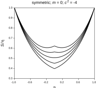
A trial-and-error process, using c2 = 1, as implied by eq 5, converges to Λ = 0.3486. Figure 2 shows the first stages of such an iteration, as reflected by the shape of f(η). We repeat the process for decreasing values of c2. The search can be automated, using a simple root-seeking algorithm such as the bisection method. Since we intend to use the functional relation between c2 and Λ to solve the radial equation, we need about a dozen pairs of values of these parameters. While it would be possible to find the Λ that corresponds to an arbitrary value of c2 by interpolation, we find it more conve- nient to fit a fourth-degree polynomial to these data by a linear least squares method. In the united atom limit, D = 0 so that c2 = 0 and Λ = 0, as befits an s state. Therefore, the fitting polynomial should appear as
Λ = a1(c2) + a2(c2)2 + a3(c2)3 + a4(c2)4 (13) The coefficients, determined over the range 1 ≥ c2 ≥ 35—
which allows 0 ≤ D ≤ 12, a convenient span of internuclear distances—are
a1 = 0.3127477; a2 = 0.0231669 a3 = 0.0005110; a4 = 0.0000045
The first excited state will again be axially symmetric, but will have an odd f. At large internuclear separation, its energy should be close to that of a 1s hydrogen atom (E ≅ 1) while tending to that of a 2p state (E ≅ 1) in the united atom limit (ᐉ = 1, one node). The electronic energy should thus be rather insensitive to D. Using c2 = 1, we discover a solu- tion for Λ = 1.393205 . A typical search for an eigenvalue is shown in Figure 3. We track this root for decreasing c2 and finally fit a polynomial to the results. The constant term must be a0 = 2, since Λ converges to the value ᐉ(ᐉ + 1) of a 2p state. Λ is observed to be an almost linear function of c2, so
Figure 2. Shooting toward an eigenvalue of the angular equation:
the symmetric case. Plots of S(η) are shown with, from top to bottom, Λ = 1.8, 1.7, 1.6, 1.5, 1.4. The best value is 1.59449.
S/η
η
1.0
0.9
0.8
0.7
0.6
0.5
0.4
0.3
-1.0 -0.6 -0.2 0.2 0.6 1.0
symmetric; m = 0; c2 = -4
that a cubic was chosen. The coefficients for the range 1 ≥ c2 ≥ 35 are
a0 = 2.000000; a1 = 0.6043499 a2 = 0.0061888; a3 = 0.0000589
The angular part of the wave function for any other state of the HMI can be found using this procedure. In order to gain time, values of c2 and Λ could be read from the tables of Abramovitz and Stegun, the computer being used only to obtain the wave function.
The Radial Equation
We seek solutions of eq 7, using a process similar to that of the last section. Here again, the equation seems to blow up at ξ = 1. The cure should by now be familiar. We shift the origin, putting ξ = 1 + u, and look for a solution of the form R(ξ) = ξp(a0 + a1ξ + a2ξ + …). The indicial equation is the same as previously and the index p is equal to |m|/2. Intro- ducing the new function g(ξ) by
R(ξ) = g(ξ)(ξ2 – 1)m/2 (14) we find that g(ξ) must be a solution of
(ξ2–1)g′′+ 2(m+1)ξg′+[2Dξ + c2ξ2 +m(m+1) – Λ]g = 0 (15) We again solve this differential eigenvalue problem by the shooting method. Boundary conditions at ξ = 1 are g(1)=1, which ensures a smooth joining of S and R along the ξ axis, and a value of g′(1) derived from the differential equation
g′ 1 =2D+c2+m m+ 1 –Λ
2m+ 1 (16)
We first choose a value of D. Then, we replace Λ by one of the polynomial expressions in c2 found in the previous subsection. Equations 15 and 16 now comprise a single un- known parameter, c2 or E. The domain of ξ being infinite, we choose a cutoff distance, ξmax ≅ 10, where we require that
|g(ξmax)| ≅ 0. The progress of a typical search is shown graphi- cally in Figure 4, as plots of the functions g(ξ).
The process is repeated for several D values in order to build an energy versus internuclear distance curve, and for the two lower states, symmetric and antisymmetric.
Accuracy
A general theory of the accuracy of shooting algorithms is available (19), but is beyond the scope of this paper. We will limit ourselves to some empirical remarks. The computations were run in double precision (roughly 13-digit accuracy). For the angular equation, we recover the results tabulated by Abramowitz and Stegun (15) (6-digit accuracy) provided the integration step is not larger than 104. The least-squares fit introduces some error (2 × 10⁴ energy units or 3 meV). If necessary, this error can be reduced by interpolating on a finer grid. The eigenvalues of the radial equation are not so well defined, mainly because we use a cutoff distance. Tests with increasing cutoffs show that the energy should be accurate to four digits if an exact value of Λ is used.
Some Results
The symmetric, lowest-energy state is usually designated as the molecular 1σg state. The correlated state in the united atom limit (1s) may also be mentioned. The antisymmetric wave function belongs to the 1σu state (sometimes called 2pσu).
The energies of these levels are shown as functions of D in Figure 5. We recall that the limiting values for D→0 are 4 and 1 Ry, respectively and 1 Ry for D→∞. The total molecular energy is obtained by adding the coulombic re- pulsion between the nuclei (2/D) to the previous quantities.
This is shown in Figure 6. The 1σg state has a minimum for D= De≅ 2, with a binding energy of 1.2 Ry. The very ac- curate calculations of Schaad and Hicks (9) give De = 1.9972, for a total energy of 1.205269238 Ry. In contrast, the energy of the 2pσu level is seen to be monotonically decreasing; this state is nonbonding or dissociative.
Figure 4. Searching for an eigenvalue of the radial equation. Func- tion R(ξ) with, from bottom to top, E = 2.1, 2.2, 2.202, 2.205, 2.21, 2.3 Ry. The best value is 2.20218 Ry.
R(ξ)
ξ
1 2 3 4 5 6 7 8 9 10
1.0
0.6
0.2
-0.2
-0.6
-1.0
symmetric; m = 0; D = 2
Figure 3. Search for an eigenvalue of the angular equation: the antisymmetric case. S as function of η with, from outside to inside, Λ = 1.3, 1.5, 1.7, 1.8. The most accurate value is 1.83105.
.
S(η)
η
1.0
0.6
0.2
-0.2
-0.6
-1.0
-1.0 -0.6 -0.2 0.2 0.6 1.0
antisymmetric; m = 0; c2 = -6
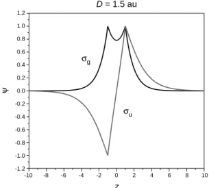
The complete wave functions are products of the relevant R(ξ) and S(η) factors. Along the molecular axis, as explained previously, ψ =R(ξ) on the right of B, ψ =S(η) between A and B, and ψ = ±R(ξ) to the left of A, the sign being chosen ac- cording to the state symmetry. Figure 7 shows ψ for D = 1.5.
Rather than displays of ψ(ξ,η), we find it more informative to plot the electron density, |ψ|2, as in Figures 8 and 9. These demonstrate rather strikingly the surplus of negative charge in the internuclear region, responsible for bonding, and the nodal plane of the antibonding orbital.
The HMI may also be studied within the LCAO–MO formalism. The simplest wave function, a linear combination of 1s atomic orbitals, leads to a binding energy of 1.13 Ry. It is only when about 100 basis functions are included that the energy accuracy becomes comparable to that of the present approach. Ready-made software for these computations may be found on the Internet (20, 21).
Conclusion
We have shown how a well-known but rather involved quantum mechanical problem can be completely solved numerically, using free software and a desktop computer. We found that the main difficulty in this undertaking was the comprehension of the equations and of the respective roles of
Figure 6. Total energy of the HMI; units and conventions are those of Figure 5.
Total Energy / (13.6 eV)
Internuclear Distance / (0.529Å)
0.0
-0.2
-0.4
-0.6
-0.8
-1.0
-1.2
-1.4
0 1 2 3 4 5 6 7 8 9 10
Figure 7. A cross section along the internuclear axis of the wave functions for D = 1.5. Black line: σg symmetric state. Gray line: σu
antisymmetric state.
Figure 5. Electronic energy of the HMI (in units of 13.6 eV) as a function of the internuclear distance (in units of 0.529 Å). Diamonds:
bonding σg state, stars: antibonding σu state.
Electronic Energy / (13.6 eV)
Internuclear Distance / (0.529Å )
-1.0 -1.2 -1.4 -1.6 -1.8 -2.0 -2.2 -2.4 -2.6 -2.8 -3.0 -3.2
0 1 2 3 4 5 6 7 8 9 10
Figure 8. Plot of the electron density |ψ|2 (normalized to ψ(1,1)=1) for the σg bonding state. Coordinates in units of 0.529 Å.
ψ2
-3
0 1.0
0.5
0.0
3 -3
0
3
z x
Figure 9. Plot of the electron density |ψ|2 (normalized to ψ(1,1)=1) for the σu antibonding state. Coordinates in units of 0.529 Å.
-3 -3
1.0
0 0 3
0.5
3 0.0
ψ2
z x
D = 1.5 au
ψ
σg
σu
z
-10 -8 -6 -4 -2 0 2 4 6 8 10
-1.2 -1.0 -0.8 -0.6 -0.4 -0.2 0.0 0.2 0.4 0.6 0.8 1.0 1.2
the various parameters. Running the programs for different values of D, Λ, and E provides valuable insight. Several extensions of these calculations are possible. Higher states of the HMI can be investigated. As shown by Wilson and Gallup (22), heteronuclear diatomic ions are amenable to this formalism. The HMI is currently the subject of active theoretical (23) and experimental investigations (24). Some conclusions of the simple treatment have been proven to be incorrect. Particu- larly, the 2pσu state is now known to possess a shallow long- range potential minimum (24).
Literature Cited
1. Pauling, L.; Wilson, E. B. Introduction to Quantum Mechanics;
McGraw-Hill: New York, 1935; pp 326–345.
2. Burrau,Ø.DanskeVidenskab.Selskab,Mat-Fys.Medd.1927,7(14).
3. Teller, E. Z. Phys. 1930, 61, 458–480.
4. Hylleraas, E. A. Z. Phys. 1931, 71, 739-763.
5. Jaffé, G. Z. Physica 1934, 87, 535–544.
6. Bates, D. R.; Ledsham, K.; Stewart, A. L. Philos. Trans. R. Soc.
London, Ser. A 1953, A246, 215–240.
7. Wind, H. J. Chem. Phys. 1965, 42, 2371–2373.
8. Peek, J. M. J. Chem. Phys. 1965, 43, 3004–3006.
9. Schaad, L. J.; Hicks, W. V. J. Chem. Phys. 1970, 53, 851–852.
10. Slater, J. C. Quantum Theory of Molecules and Solids, Vol. 1;
McGraw-Hill: New York, 1963; pp 1–11, 247–251.
11. Levine, I. N. Quantum Chemistry, 4th ed.; Prentice Hall:
Englewood Cliffs, NJ, 1991; Chapter 13.
12. Press, W. H.; Teukolsky, S. A.; Vetterling, W. T.; Flannery B. P.
Numerical Recipes in C. The Art of Scientific Computing;
Cambridge University Press: New York, 1992; Chapter 17.
13. Morse, P. M.; Feshbach, H. Methods of Theoretical Physics;
McGraw-Hill: New York, 1953; Vol. 2, Chapter 10.
14. Arfken, G. Mathematical Methods for Physicists; Academic:
New York, 1968; Chapter 2.
15. Abramowitz, M.; Stegun, I. A. Handbook of Mathematical Functions; Dover: New York, 1972; pp 752–769.
16. Flammer, C. Spheroidal Wave Functions; Stanford University Press: Stanford, CA 1957.
17. Thompson, W. J. Comp. Sci. Eng. 1999, 1, 84–87.
18. Boyce, W. E.; DiPrima, R. C. Elementary Differential Equations and Boundary Value Problems, 4th ed.; Wiley: New York, 1986;
Chapter 11.
19. Pryce, J. D. Numerical Solution of Sturm–Liouville Problems;
Clarendon: Oxford, 1993.
20. Gordon Quantum Theory Group. GAMESS; http://www.msg.
ameslab.gov/GAMESS/summary.html; University of Iowa: Ames;
accessed Oct 2001.
21. High-Performance Computational Chemistry Group, EMSL, PNNL. NWChem; http://www.emsl.pnl.gov:2080/docs/nwchem/
nwchem.html (accessed Nov 2001).
22. Wilson, L. Y. ; Gallup, G. A. J. Chem. Phys. 1966, 45, 586–590.
23. Taylor, J. M.; Yan, Z.-C.; Dalgarno, A.; Babb J. F. Mol. Phys.
1999, 97, 25–35.
24. Leach, C. A.; Moss, R. E. Annu. Rev. Phys. Chem. 1995, 46, 55–82.
25. Scilab Group. Scilab 2.5; 1999; http://www-rocq.inria.fr/scilab (accessed Oct 2001).
Appendix: Computational Details
All computations reported in this article were done using the free software Scilab (25), which incorporates routines to solve initial value problems and to plot graphs of functions of one or several variables.
Algorithms for solving differential equations operate on first- order equations or systems of equations. The first task in computing R(ξ) and S(η) consists in transforming the relevant second-order equations into systems of two first-order equations. This is easily done at the price of a change of function. Consider the case of R;
it is determined through the auxiliary function g(ξ). We introduce the vector of unknowns [z1(ξ), z2(ξ)] defined as z1(ξ) = g(ξ) and z2(ξ) = g′(ξ). Equation 15 takes the form
z1(ξ)′= z2(ξ)
z2 ξ ′= 2m+ 1ξz2ξ + 2Dξ+c2ξ2+m m+ 1 –Λz1ξ ξ2– 1
The program operates on discrete values. We choose a step size, h, and initial and final values of ξ and create a vector of abscissas {Xk}, numbered from 1 to n. The program will generate approximations to z1 and z2, in the form of two arrays Z1,k and Z2,k, k = 1, …, n. The program should start at X1 = 1, where the initial conditions (see eq 16) apply. This leads to a division by zero in eq 15, so that we start the actual computation at X2 = h, using the known slope at X1 to set the values of Z1,2 and Z2,2. At the end, we insert the correct values of Z1,1 and Z2,1.
The definition and solving of eq 15 are taken care of in a few lines of code by Scilab. A double slash (//) indicates a comment. If z is a vector, z′ is the transposed vector. Input and output state- ments have been deleted.
//radial equation in terms of vector z deff(“[zdot]=g(x,z)”,...
“zdot=[z(2); (-2*(m+1)*x*z(2)-(2*D*x+m*(m+1)- L+c2*x*x)*z(1))/(x*x-1)]”)
step = 0.001;
x0=1+step;
x=x0:step:10;//abscissas,starting atpointnextto 1.
c2=D*D*E/4;
//L(c) for an antisymmetric f L=(((-6.373E-7*c2-0.0001053)*c2-
0.0071351)*c2+0.5992722)*c2+1.9994397;
//initial conditions
slope = -(-L+m*(m+1)+2*D+c2)/(m+1)/2;
z0=[1+step*slope,slope]’;
//solve differential equation z=ode(z0,x0,x,g);
//compute R from z temp=x.*x-1;
temp=temp.^(m/2);
//extract values of g zz=temp.*z(1,:);
//insert missing values zz=[1,zz];xt=[1,x];
According to the shooting method, we run this program for various values of E while watching Z1,n. We stop when this quan- tity is smaller than a prescribed threshold.
The code needed to solve the angular eq 10 is quite similar, except that the two cases of even and odd f must be considered separately and we shoot from both ends of the interval, inward, and try to comply with eq 12.
The same software incorporates a least-squares fitting routine, allowing an easy computation of the polynomial regression of Λ versus c2.