DOI:10.1017/S0013091516000420
SPLITTING NUMBERS OF LINKS
JAE CHOON CHA1,2, STEFAN FRIEDL3∗ AND MARK POWELL4
1Department of Mathematics, POSTECH, Pohang 790–784, Republic of Korea (jccha@postech.ac.kr)
2School of Mathematics, Korea Institute for Advanced Study, Seoul 130–722, Republic of Korea
3Mathematisches Institut, Universit¨at zu K¨oln, 50931 K¨oln, Germany (sfriedl@gmail.com)
4D´epartement de Math´ematiques, Universit´e du Qu´ebec `a Montr´eal, Montr´eal, QC, Canada (mark@cirget.ca)
(Received 18 December 2013)
Abstract The splitting number of a link is the minimal number of crossing changes between different components required, on any diagram, to convert it to a split link. We introduce new techniques to compute the splitting number, involving covering links and Alexander invariants. As an application, we completely determine the splitting numbers of links with nine or fewer crossings. Also, with these techniques, we either reprove or improve upon the lower bounds for splitting numbers of links computed by Batson and Seed using Khovanov homology.
Keywords:splitting numbers of links; covering links; Alexander polynomial 2010Mathematics subject classification:Primary 57M25; 57M27; 57N70
1. Introduction
Any link inS3can be converted to the split union of its component knots by a sequence of crossing changes between different components. Following Batson and Seed [2], we define the splitting number of a link L, denoted by sp(L), as the minimal number of crossing changes in such a sequence.
We present two new techniques for obtaining lower bounds for the splitting number.
The first approach uses covering links, and the second method arises from the multivari- able Alexander polynomial of a link.
Our general covering link theorem is stated as Theorem 3.2. Theorem 1.1 gives a special case that applies to two-component linksLwith unknotted components and odd linking number. Note that the splitting number is equal to the linking number modulo 2. If we take the two-fold branched cover ofS3 with branching set a component ofL, then the preimage of the other component is a knot inS3, which we call atwo-fold covering knot
∗ Present address: Universit¨at Regensburg, Fakult¨at f¨ur Mathematik, 93053 Regensburg, Germany
c 2017 The Edinburgh Mathematical Society 587
ofL. Also recall that theslice genusof a knotKinS3is defined to be the minimal genus of a surfaceF smoothly embedded inD4such that ∂(D4, F) = (S3, K).
Theorem 1.1. Suppose thatLis a two-component link with unknotted components.
Ifsp(L) = 2k+ 1, then any two-fold covering knot ofLhas slice genus at mostk.
Theorem 3.2 also has other useful consequences, given in Corollaries 3.5 and 3.6, dealing with the case of even linking numbers, for example. Three covering link arguments that use these corollaries are given in§7.
Our Alexander polynomial method is efficacious for two-component links when the linking number is 1 and at least one component is knotted. By looking at the effect of a crossing change on the Alexander module, we obtain the following result.
Theorem 1.2. Suppose thatL is a two-component link with Alexander polynomial ΔL(s, t). Ifsp(L) = 1, thenΔL(s,1)·ΔL(1, t)dividesΔL(s, t).
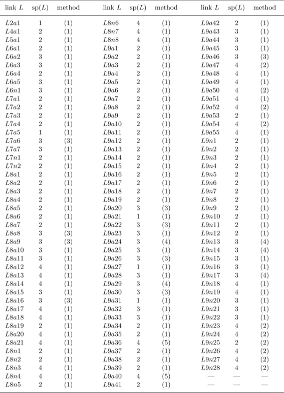
We will use elementary methods explained in Lemma 2.1 and our techniques from covering links and Alexander polynomials to obtain lower bounds on the splitting number for links with nine or fewer crossings. Together with enough patience with link diagrams, this is sufficient to determine the splitting number for all of these links. Our results for links with up to nine crossings are summarized by Table 3 in§6.
In [2], Batson and Seed defined a spectral sequence from the Khovanov homology of a link L that converges to the Khovanov homology of the split link with the same components asL. They showed that this spectral sequence gives rise to a lower bound on sp(L), and by computing it for links with up to 12 crossings, they gave many examples for which this lower bound is strictly stronger than the lower bound coming from linking numbers. They determined the splitting number of some of these examples, while some were left undetermined.
We revisit the examples of Batson and Seed and show that our methods are strong enough to recover their lower bounds. Furthermore, we show that for several cases our methods give more information. In particular, we completely determine the splitting numbers of all the examples of Batson and Seed. We refer the reader to §5 for more details.
Organization of the paper
We start out, in§2, with some basic observations on the splitting number of a link. In
§3.1 we prove Theorem 3.2, which is a general result on the effect of crossing changes on covering links, and then we provide an example in§3.2. We give a proof of Theorem 1.2 in
§§4.1 and 4.2 and we illustrate its use with an example in§4.3. The examples of Batson and Seed are discussed in§5, with§5.1 focusing on examples that use Theorem 1.2, and
§5.2 on examples that require Theorem 1.1. A three-component example of Batson and Seed is discussed in §5.3. Next, our results on the splitting numbers of links with nine crossings or fewer are given in§6, with some particular arguments used to obtain these results described in§7.
L2
L1 L3
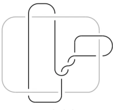
Figure 1. The linkL9a54.
2. Basic observations
A link is split if it is a split union of knots. We recall from the introduction that the splitting numbersp(L) of a linkLis defined to be the minimal number of crossing changes that one needs to make onL, each crossing change between different components, in order to obtain a split link.
We note that this differs from the definition of ‘splitting number’ that occurs in [1,17];
in these papers, crossing changes of a component with itself are permitted.
Given a linkL we say that a non-split sublink with all of the linking numbers zero is obstructive. (All obstructive sublinks that occur in the applications of this paper will be Whitehead links.) We then definec(L) to be the maximal size of a collection of distinct obstructive sublinks ofLsuch that any two sublinks in the collection have at most one component in common. Note thatcis zero for trivial links.
As another example consider the linkL9a54 shown in Figure 1. The sublinkL1L3is an unlink, while bothL1L2andL2L3are Whitehead links, and hence are obstructive.
Thus,c(L) = 2.
Finally, we discuss the linkJ in Figure 17. It has four componentsJ1,J2,J3,J4, and J1∪J3andJ2∪J4 each form a Whitehead link. It follows thatc(J) = 2.
In practice it is straightforward to obtain lower bounds forc(L). In most cases it is also not too hard to determinec(L) precisely.
Now we have the following elementary lemma.
Lemma 2.1. LetL=L1 · · · Lm be a link. Then sp(L)≡
i>j
lk(Li, Lj) mod 2 and
sp(L)
i>j
|lk(Li, Lj)|+ 2c(L).
Proof . Given a linkL we write
a(L) =
i>j
|lk(Li, Lj)|.
Note that a crossing change between two different components always changes the value ofaby precisely 1. Sinceaof the unlink is zero we immediately obtain the first statement.
If we do a crossing change between two components with non-zero linking number, thenagoes down by at most 1, whereascstays the same or increases by 1. On the other hand, if we do a crossing change between two components with zero linking number, thenagoes up by 1 andcdecreases by at most 1, since the two components belong to at most one obstructive sublink in any maximal collection whose cardinality realizesc(L).
It now follows thata(L) + 2c(L) decreases with each crossing change between different
components by at most 1.
The right-hand side of the second inequality is greater than or equal to the lower bound blk(L) of [2,§5]. In some cases the lower bound coming from Lemma 2.1 is stronger. For example, letLbe two split copies of the Borromean rings. For thisLwe have c(L) = 2, giving a sharp lower bound on the splitting number of 4, whereasblk(L) = 2.
3. Covering link calculus
In this section, first we prove our main covering link result, Theorem 3.2, showing that covering links can be used to give lower bounds on the splitting number. Then we show how to extract Theorem 1.1 and three other useful corollaries from Theorem 3.2. In§3.2 we present an example of this approach.
3.1. Crossing changes and covering links
The following definition is a special case of the notion of a covering link occurring, for example, in [14, Method 5] and [5].
Definition 3.1. LetL=L1· · ·Lmbe anm-component link withLiunknotted. We denote the double branched cover ofS3with branching set the unknotLibyp:S3→S3. We refer top−1(L\Li) as thetwo-fold covering link ofL with respect toLi.
We note that a choice of orientation of a link induces an orientation of its covering links.
In the theorem below we use the term internal band sum to refer to the operation on an oriented link L described as follows. The data for the move is an embedding f: D1×D1 ⊂ S3 such that f(D1 ×D1)∩L = f({−1,1} ×D1), the orientation of f({−1}×D1) agrees with that ofL, and the orientation off({1}×D1) is opposite to that ofL. The output is a new oriented link given by (L\f({−1,1} ×D1))∪f(D1× {−1,1}), after rounding corners. The new link has the orientation induced fromL.
Theorem 3.2. LetL=L1 · · · Lmbe anm-component link and suppose thatLiis unknotted for some fixedi. Fix an orientation ofL. Suppose thatLcan be transformed to a split link byα+β crossing changes involving distinct components, whereαof these involveLi andβ of these do not involveLi. Then the two-fold covering linkJ ofLwith respect toLican be altered by performingαinternal band sums and2βcrossing changes between different components to the split union of2(m−1)knots comprising two copies ofLj for eachj=i.
L2
L1 J L~1 J
Figure 2. The effect of a crossing change on a two-fold covering link where one component is the branching set.
Proof . We may assume that i = 1. We begin by investigating the effect of crossing changes on the two-fold covering link with respect to the first componentL1of a linkL.
Type A.First we consider crossing changes between the branching componentL1and another component, say L2. Such a crossing change lifts to a rotation of the preimage J of L2 around the lift L1 of L1, as shown in Figure 2. The top-left and middle-left diagrams show a link before and after a crossing change, in a cylindrical neighbourhood that contains an interval from each of L1 and L2. To branch over L1, which is the component running down the centre of the cylinders, cut along the surface that is shown in the diagrams. The results of taking the top-left and middle-left diagrams, cutting, and gluing two copies together, are shown in the top-right and middle-right diagrams, respectively.
After forgetting the branching set, the same effect on the lift of L2 can be achieved by adding a band to J (see the bottom diagram of Figure 2). By ignoring the band, we obtain the top-right diagram with the branching component removed. If we instead use the band to make an internal band sum, we obtain the middle-right diagram with the branching set removed. Note that this band is attached to J in such a way that orientations are preserved. This holds no matter what choice of orientations was made
forL. Thus, we see that a crossing change betweenL1andL2corresponds to an internal band sum on the covering link.
Type B.Consider a crossing change that does not involveL1, say betweenL2 andL3. Such a crossing change can be realized by ±1 Dehn surgery on a circle that has zero linking number withLand that bounds an embedded disc, sayD, inS3 that intersects L in two points of opposite signs, one point ofL2 and one point ofL3. By performing the Dehn surgeries, and then taking the branched cover overL1, we produce the covering link of the link obtained by the crossing change.
Note that the preimage of the disc D in the double branched cover consists of two disjoint discs, each of which intersects the covering link transversally at two points with opposite signs, one point of the preimage ofL2 and one point of the preimage ofL3. As an alternative construction, we can take the branched cover and then perform±1 Dehn surgeries along the boundary circles of the preimage discs. This gives the same covering link. From this it follows that a single crossing change betweenL2 and L3 corresponds to two crossing changes on the covering link.
Note that when there is more than one crossing change, of either type, the correspond- ing surgery discs and bands associated with the covering link are disjoint.
Recall that the linkLcan be altered to become the split union ofmknotsL1, . . . , Lm
by α crossing changes of Type A and β crossing changes of Type B. By the above arguments, the two-fold covering link ofL with respect to the first componentL1 can be altered to become the corresponding covering link of the split link, which is the split unionL2L2 · · · LmLm, byαinternal band sums and 2β crossing changes.
In the following result,g4(K) denotes the slice genus of a knotK in S3, namely, the minimal genus of a smoothly embedded connected oriented surface inD4whose boundary isK.
Corollary 3.3. Under the same hypotheses as Theorem 3.2, the two-fold covering link ofLwith respect toLi bounds a smoothly embedded oriented surfaceF inD4that has no closed components and has Euler characteristic
χ(F) = 2(m−1)−α−4β−4
k=i
g4(Lk).
In addition, if there is some j = i such that each Lk with k = j is involved in some crossing change withLj, thenF is connected.
Proof . Once again we may assume that i= 1. LetJ be the two-fold covering link of Lwith respect toL1.
An internal band sum can be inverted by performing another band sum, while the inverse of a crossing change is also a crossing change. Hence, by Theorem 3.2 we can also obtain the covering linkJ from the split unionL2L2 · · · LmLm by performing αinternal band sums and 2β crossing changes.
Choose surfaces Vj embedded in D4 with ∂Vj = Lj and genus g4(Lj). Take a split unionV2V2 · · · VmVm inD4. The boundary of these surfaces is the split union
L2L2 · · · LmLm. The covering linkJ can be realized as the boundary of a surface obtained from the split union of the surfaces by attachingαbands and 2β clasps inS3. As pointed out in the proof of Theorem 3.2, the surgery discs and bands associated with crossing changes are disjoint. Pushing slightly intoD4, we obtain an immersed surface inD4bounded byJ; each clasp gives a transverse intersection. As usual, we remove the intersections by cutting out a disc neighbourhood of the intersection point from each sheet and gluing a twisted annulus that is a Seifert surface for the Hopf link. This gives a smoothly embedded oriented surfaceF inD4 bounded by the covering linkJ. Note that each band attached changes the Euler characteristic of the surface by −1, while each twisted annulus used to remove an intersection point changes the Euler characteristic by−2. Therefore, the resulting surfaceF has Euler characteristic
χ(F) =
m
k=2
2·(1−2g4(Vk))−α−4β, which is equal to the claimed value.
The final conclusion of the corollary states (wheni= 1) that F is connected if there is somej= 1 such that eachLk withk=j is involved in some crossing change withLj. To see this, observe that a crossing change involvingLj and L1 joins the two copies of Vj; a crossing change involving Lj and Lk with j, k 2 joins one of the two copies of Vj to one of the two copies ofVk and joins the other copy ofVj to the other copy ofVk.
Under the hypothesis, it follows thatF is connected.
Corollary 3.3 has some useful consequences of its own. Considering the case in which m= 2,α= 2k+ 1,β = 0 andg4(Lk) = 0, we obtain Theorem 1.1.
Theorem 1.1. Suppose thatLis a two-component link with unknotted components.
Ifsp(L) = 2k+ 1, then any two-fold covering knot ofLhas slice genus at mostk.
Remark 3.4.
(1) In the proof of Corollary 3.3, when β = 0, we construct an embedded surface F without local maxima. Therefore, in order to show, using Theorem 1.1, that a link of linking number 1 with unknotted components has splitting number at least 3, it suffices to show that the covering link is not a ribbon knot.
(2) Different choices of orientation on a link J can change the minimal genus of a connected surface thatJbounds inD4. Since the splitting number is independent of orientations, in applications we will choose the orientation that gives the strongest lower bound. This remark will be relevant in§5.3.
(3) If L is a non-split two-component link, then the surface F of Corollary 3.3 is automatically connected, by the last sentence of that corollary.
The following is another useful consequence of Corollary 3.3.
Figure 3. The linkL9a30.
Corollary 3.5. Suppose thatLis a two-component link with unknotted components andsp(L) = 2. Then any two-fold covering link ofL is weakly slice; that is, bounds an annulus smoothly embedded inD4.
Proof . First note that a two-fold covering link has two components, since the linking number is even by Lemma 2.1. Applying Corollary 3.3 withm = 2,α= 2, β = 0 and
g4(Lk) = 0, the conclusion follows.
We state one more corollary to Theorem 3.2. Let spi(L) be the minimal number of crossing changes between distinct components not involving Li required to transform L to a split link. By convention, spi(L) is infinite if we must make a crossing change involvingLi in order to splitL.
Corollary 3.6 (see Kohn [14, Method 5]). For a linkL=L1 · · · Lmand its two-fold covering linkJ with respect toLi, we havespi(L) 12sp(J).
Proof . This follows from Theorem 3.2 withα= 0.
We remark that the above results generalize ton-fold covering links in a reasonably straightforward manner. One can also draw analogous conclusions when the branching component is knotted. We do not address these generalizations here, since the results stated above are sufficient for the applications considered in this paper.
3.2. An example of the covering link technique
To illustrate the use of the method developed in§3.1, we now apply it to prove that the splitting number of the two-component linkL9a30 is 3. More applications of Theorem 1.1 and Corollaries 3.5 and 3.6 will be discussed later (see, for example,§§5.2, 5.3, 6 and 7). In this paper, we use the link names employed in the LinkInfo database [7]. The linkL9a30 is shown in Figure 3. It is a two-component link of linking number 1 with unknotted components. Recall that the splitting number is determined modulo 2 by the linking number by Lemma 2.1. It is easy to see from Figure 3 that three crossing changes suffice, so the splitting number is either 1 or 3.
To see that sp(L9a30)= 1, we take a two-fold cover branched over one of the com- ponents, and check that the resulting knot is not slice. Figure 4 shows the result of an
Figure 4. Left: the linkL9a30 after an isotopy to prepare for taking the cover branching over the most obviously unknotted component. Right: the knot that arises as the covering link after taking a two-fold branched cover and deleting the branching set.
Figure 5. The covering knot on the right of Figure 4 after an isotopy.
isotopy that was made in preparation for taking a branched cover on the left, and the knot obtained as the preimage of L9a30 after deleting the preimage of the branching component on the right.
The knot on the right of Figure 4 after a simplifying isotopy is shown in Figure 5;
it is a twist knot with a negative clasp and seven positive half-twists. This knot is well known not to be a slice knot, a fact that was first proved by Casson and Gordon [3,4].
Therefore, by Theorem 1.1, the splitting number ofL9a30 is at least 3, as claimed.
4. Alexander invariants
In this section we will recall the definition of Alexander modules and polynomials of oriented links. We then show how Alexander modules are affected by a crossing change, which then allows us to prove Theorem 1.2.
4.1. Crossing changes and the Alexander module
Throughout this section, given an orientedm-component linkL, the oriented meridians are denoted byμ1, . . . , μm. Note thatμ1, . . . , μm give rise to a basis forH1(S3\νL;Z).
We will henceforth use this basis to identifyH1(S3\νL;Z) withZm. LetRbe a subring of Cand let ψ:Zm → F be a homomorphism to a free abelian group. We denote the induced map
π1(S3\νL)→H1(S3\νL;Z) =Zm ψ−→F
byψ as well. We can then consider the corresponding Alexander module H1ψ(S3\νL;R[F])
and the order of the Alexander module is denoted by
ΔψL∈R[F] = ordR[F](H1ψ(S3\νL;R[F])).
(We refer the reader to [9] for the definition of the order of an R[F]-module.) If ψ is the identity, then we drop ψ from the notation and we obtain the usual multivariable Alexander polynomialΔL.
Note that what we term the Alexander module has also been called the ‘link module’
in the literature (see, for example, [11]). The following proposition relates the Alexander modules of two oriented links that differ by a crossing change.
Proposition 4.1. LetLand L be two orientedm-component links that differ by a single crossing change. LetRbe a subring ofCand letψ:Zm→F be a homomorphism to a free abelian group. Then there exists a diagram
R[F]
))S
SS SS SS
SS R[F]
uukkkkkkkkk
M
vvlllllll
((R
RR RR RR R H1ψ(S3\νL;R[F])
vvmmmmmmm
H1(S3\νL;R[F])
((Q
QQ QQ QQ Q
0 0
whereM is someR[F]-module and where the diagonal sequences are exact.
The formulation of this proposition is somewhat more general than what is strictly needed in the proof of Theorem 1.2. We hope that this more general formulation will be applicable, in future work, to the computation of unlinking numbers; see the beginning of§6 for the definition of the unlinking number of a link.
Proof . We writeX =S3\νLandX =S3\νL. We pick two open disjoint discsD1 andD2 in the interior ofD2and we write
B= (D2\(D1∪D2))×[0,1],
S= (D2\(D1∪D2))× {0,1} ∪∂D2×{0,1}S1×[0,1].
Put differently,Sis the ‘top and bottom boundary’ ofBtogether with the outer cylinder S1×[0,1].
SinceL and L are related by a single crossing change, there exists a subset Y of X and continuous injective mapsf:B→X andf:B→Xwith the following properties:
(1) X =Y ∪f(B) andY ∩f(B) =f(S), (2) X=Y ∪f(B) andY ∩f(B) =f(S).
We can now state the following claim.
Claim 4.2. There exists a short exact sequence
R[F]→H1ψ(Y;R[F])→H1ψ(X;R[F])→0.
By a slight abuse of notation we now writeB=f(B) andS=f(S). We then consider the Mayer–Vietoris sequence
· · · →H1ψ(S;R[F])−−−−→i∗⊕j∗ H1ψ(B;R[F])⊕H1ψ(Y;R[F])→H1ψ(X;R[F])
→H0ψ(S;R[F])−−−−→i∗⊕j∗ H0ψ(B;R[F])⊕H0ψ(Y;R[F]), wherei:S →B and j: S→Y are the two inclusion maps. We need to study the rela- tionships between the homology groups ofSandB. We make the following observations.
By [10, §VI.3] we have the following commutative diagram:
H0ψ(S;R[F])
∼=
//Hψ0(B;R[F])
∼=
R[F]/{ψ(g)v−v}v∈R[F], g∈π1(S) //R[F]/{ψ(g)v−v}v∈R[F], g∈π1(B)
Here the horizontal maps are induced by the inclusion S → B and the vertical maps are isomorphisms. The mapi∗:π1(S)→π1(B) is surjective; it follows that the bottom horizontal map is an isomorphism. Hence, the top horizontal map is also an isomorphism.
The above Mayer–Vietoris sequence thus simplifies to the following sequence:
H1ψ(S;R[F])−−−−→i∗⊕j∗ H1ψ(B;R[F])⊕H1ψ(Y;R[F])→H1ψ(X;R[F])→0.
We note that the spaceB is homotopy equivalent to a wedge of two circlesmandn.
Furthermore,S is homotopy equivalent to the wedge ofm,nand another curvem that is homotopic tominB. By another slight abuse of notation we now replaceBandS by these wedges of circles and we viewB andS as CW-complexes with precisely one 0-cell in the obvious way. We denote byp: ˜S→S andp: ˜B →B the coverings corresponding to the homomorphismsπ1(S)→π1(B)→π1(X)−→ψ F. Note that we can and will view ˜B as a subset of ˜S. We now pick preimages ˜m, ˜nand ˜mofm,nandm under the covering mapp: ˜S →S. Note that{m,˜ n˜} is a basis for C1(B;R[F]) =C1( ˜B) and{m,˜ ˜n,m˜}is a basis for C1(S;R[F]) =C1( ˜S). The kernel of the map C1(S;R[F])→ C1(B;R[F]) is
given byR[F]·(m−m). We thus obtain the following commutative diagram of chain complexes with exact rows:
0 //R[F]·(m−m) //
C1(S;R[F])
i∗ //C1(B;R[F]) //
0
0 //C0(S;R[F]) i∗ //C0(B;R[F]) //0 It now follows easily from the diagram, or more formally from the snake lemma, that
ker(i∗:H1ψ(S;R[F])→H1ψ(B;R[F]))∼=R[F]·(m−m) (4.1) and that
coker(i∗:H1ψ(S;R[F])→H1ψ(B;R[F])) = 0. (4.2) Finally, we consider the following commutative diagram:
R[F]·(m−m) //
H1ψ(Y;R[F]) //
⎛
⎝0 Id
⎞
⎠
H1ψ(X;R[F])
=
//0
H1ψ(S;R[F]) //H1ψ(B;R[F])⊕H1ψ(Y;R[F]) //H1ψ(X;R[F]) //0 We have already seen above that the bottom horizontal sequence is exact. It now follows from (4.1), (4.2) and a straightforward diagram chase, that the top horizontal sequence is also exact. This concludes the proof of the claim.
Precisely the same proof shows that there exists a short exact sequence R[F]→H1ψ(Y;R[F])→H1ψ(X;R[F])→0.
(UseB=f(B),S=f(S) instead ofB =f(B),S=f(S).) Combining these two short exact sequences now gives the desired result, by takingM :=H1ψ(Y;R[F]).
4.2. The Alexander polynomial obstruction
Using Proposition 4.1 we can prove the following obstruction to the splitting number being equal to 1.
Theorem 4.3. Let L be a two-component oriented link. We denote the Alexander polynomial ofLbyΔL(s, t). If the splitting number ofLequals1, thenΔL(s,1)·ΔL(1, t) dividesΔL(s, t).
Let L = J ∪K be an oriented link with splitting number equal to 1. We denote the Alexander polynomials of J and K by ΔJ and ΔK, respectively. It follows from Lemma 2.1 that the linking number satisfies |lk(J, K)| = 1. Therefore, by the Torres condition,|ΔL(1,1)|= 1 and we have that
ΔL(s,1) =ΔJ(s) and ΔL(1, t) =ΔK(t).
We can thus reformulate the statement of the theorem as saying that ifL =J ∪K is an oriented link with splitting number equal to 1, then ΔJ(s) and ΔK(t) both divide ΔL(s, t).
Proof . LetL=J∪Kbe an oriented link with splitting number equal to 1. We denote byψ:H1(S3\L;Z)→ s, t|[s, t] = 1the map that is given by sending the meridian of J to sand by sending the meridian ofKto t. We writeΛ:=Z[s±1, t±1].
In the following we also denote byψ the map H1(S3\J;Z)→ s, t|[s, t] = 1, which is given by sending the meridian of J to s. Note that with this convention we have an isomorphism
H1ψ(S3\J;Λ) =H1(S3\J;Z[s±1])⊗Z[s±1]Λ and we obtain that
ordΛ(H1ψ(S3\J;Λ)) =ΔJ(s). (4.3) Similarly, we define a mapH1(S3\K;Z)→ s, t|[s, t] = 1by sending the meridian ofK tot. We see that
ordΛ(H1ψ(S3\K;Λ)) =ΔK(t). (4.4) We denote the split link with components J and K by J K. The Mayer–Vietoris sequence forS3\(J K), which comes from splitting along the separating 2-sphereS, gives rise to an exact sequence
0→H1ψ(S3\J;Λ)⊕H1ψ(S3\K;Λ)→H1ψ(S3\(JK);Λ)
−→h H0(S;Λ)→H0ψ(S3\J;Λ)⊕H0ψ(S3\K;Λ).
We recall that by [10, §VI], for any connected space X with a ring homomorphism ψ:π1(X)→Λ, we have
H0ψ(X;Λ) =Λ/{ψ(g)v−v|v∈Λ, g∈π1(X)}.
It follows easily that H0ψ(S;Λ) ∼= Λ and that H0ψ(S3\J;Λ) and H0ψ(S3\K;Λ) are Λ-torsion. In particular, we see that the last map in the above long exact sequence has a non-trivial kernel. By the exactness of the Mayer–Vietoris sequence above, it follows that the maphhas non-trivial image.
SinceL has splitting number 1, we can do one crossing change involving bothJ and K to turn L into J K. The conclusion of Proposition 4.1 together with the above Mayer–Vietoris sequence gives rise to a diagram of maps as follows:
Λ f //M p ////
g
H1ψ(S3\L;Λ)
H1ψ(S3\J;Λ)⊕H1ψ(S3\K;Λ) //H1ψ(S3\(JK);Λ) h //Λ
where the top and bottom horizontal sequences are exact, and where the maphis non- trivial. In particular, note thatpgives rise to an isomorphismM/f(Λ)∼=H1ψ(S3\L;Λ), and thatg gives rise to an epimorphism
H1ψ(S3\L;Λ)∼=M/f(Λ)→H1ψ(S3\(JK);Λ)/(g◦f)(Λ). (4.5) Next we will prove the following claim.
Claim 4.4. The map
H1ψ(S3\J;Λ)⊕H1ψ(S3\K;Λ)→H1ψ(S3\JK;Λ)/(g◦f)(Λ) is a monomorphism.
We consider the commutative diagram
Λ
g◦f
0 //H1ψ(S3\J;Λ)⊕H1ψ(S3\K;Λ) //H1ψ(S3\(J K);Λ) h //
Λ
Hψ1(S3\(J K);Λ)
(g◦f)(Λ)
h //Λ/(h◦g◦f)(Λ) where the bottom vertical maps are the obvious projection maps. Furthermore, as above, the maphin the middle sequence is non-trivial.
We first note that the bottom-left group isΛ-torsion. Indeed, in the discussion pre- ceding the proof we saw that ΔL(s, t) = 0. This implies that the homology group H1ψ(S3\L;Λ) is Λ-torsion. But by (4.5) this also implies that the bottom-left group of the diagram isΛ-torsion.
It follows that in the square the composition of maps given by going down and then right factors through aΛ-torsion group. On the other hand, we have seen that the map h:H1ψ(S3\(JK);Λ)→Λ is non-trivial. By the commutativity of the square and by the fact that the down-right composition of maps factors through aΛ-torsion group, it now follows that the projection mapΛ →Λ/(h◦g◦f)(Λ) cannot be an isomorphism.
But this just means that the composition
Λ−−→g◦f H1ψ(S3\(JK);Λ)−→h Λ is non-trivial and, in particular, injective. Put differently, we have
im(g◦f:Λ→H1ψ(S3\(J K);Λ))∩ker(h) = 0.
By the exactness of the middle horizontal sequence, we thus see that the intersection of the images of (g◦f)(Λ) and of H1ψ(S3\J;Λ)⊕H1ψ(S3\K;Λ) inH1ψ(S3\(J K);Λ) is trivial. It follows that the map
H1ψ(S3\J;Λ)⊕H1ψ(S3\K;Λ)→H1ψ(S3\JK;Λ)/(g◦f)(Λ) is indeed a monomorphism. This concludes the proof of the claim.
K
J
Figure 6. The linkL9a29, with splitting number 3.
Before we continue with the proof we recall that if 0→A→B →C→0
is a short exact sequence ofΛ-modules, then by [9, Part 1.3.3] the orders of the modules are related by the equality
ordΛ(B) = ordΛ(A)·ordΛ(C). (4.6) We thus see, from the claim and from (4.6), (4.3) and (4.4), that
ΔJ(s)·ΔK(t)|ordΛ(H1ψ(S3\JK;Λ)/(g◦f)(Λ)).
On the other hand, it follows from (4.5) and again from (4.6) that
ordΛ(H1ψ(S3\(JK);Λ)/(g◦f)(Λ))|ordΛ(H1ψ(S3\L;Λ)).
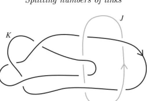
4.3. An example of the Alexander polynomial technique We consider the oriented linkL=KJ =L9a29 from Figure 6.
It has linking number 1 and it is not hard to see that one can turn it into a split link using three crossing changes between the two components. The multivariable Alexander polynomial ofLis
ΔL(s, t) =s−s2+t−st+s2t−t2+st2−s2t2+t3−st3+s2t3−t4+st4. It is straightforward to see that ΔJ(s)·ΔK(t) = 1−t+t2 does not divideΔL(s, t). It thus follows from Theorem 4.3 that the splitting number ofLis 3.
This is one of the instances of the use of the Alexander polynomial that is cited in
§6, in Table 3 (Method (4)). The other computations listed in that table as using this method are performed in a similar fashion; see the LinkInfo tables [7] for the multivariable Alexander polynomials of the other nine-crossing links, which areL9a24,L9n13,L9n14 and L9n17. Since these are two-component links of linking number 1, the Alexander polynomials of the components can be obtained by substituting either t = 1 or s = 1 into the multivariable Alexander polynomial inZ[s±1, t±1].
Figure 7. A two-component link of linking number 1 whose splitting number equals 3.
5. The examples of Batson and Seed
In [2], Batson and Seed constructed a spectral sequence from the Khovanov homology of a linkLto the Khovanov homology of the split link with the same components asL.
This spectral sequence gives rise to a lower bound on the splitting number, given by the lowest page on which their spectral sequence collapses.
Batson and Seed computed the lower bound for all links up to 12 crossings and they showed that it provides more information than basic linking number observations (see our Lemma 2.1) for 17 links. The lower bound they computed will be denoted byb(L).
One of the 17 links is a three-component link with 12 crossings, for whichb(L) = 3, while the sum of the absolute values of the linking numbers is 1. The remaining 16 links have two components and satisfy lk(L) = ±1 and b(L) = 3. One of these has 11 crossings, and 15 of these have 12 crossings. Batson and Seed determined the splitting numbers for seven links among these 17 links, while for the other 10 cases the splitting numbers are listed as being either 3 or 5. This information is given in [2, Table 3].
In this section we revisit these links to reprove or improve the results in [2]. In partic- ular, we completely determine the splitting numbers by using our methods.
5.1. Using the Alexander polynomial
We first apply our Alexander polynomial method to the examples of [2] with at least one knotted component. This will reprove their splitting number results for these links.
Before we turn to the links of [2, Table 3], we will discuss a link with 13 crossings in detail, which is also discussed in [2].
A13-crossing example
Consider the two-component linkLshown in Figure 7. It is the link denoted by2n138862 in [2].
Note that one component is an unknot and the other is a trefoil. We refer to the unknotted component asJ and to the knotted component as K. It is not hard to see thatL can be turned into a split link using three crossing changes. On the other hand, the linking number is 1, so it follows from Lemma 2.1 that the splitting number is either 1 or 3. The invariantb(L) shows that the splitting number ofLis in fact 3.
We will now use Theorem 4.3 to give another proof that the splitting number ofL equals 3. We used Kodama’s programknotGTKto show that
ΔL(s, t) =−s8t4+s7t5+ 4s8t3−5s6t5−6s8t2−9s7t3+ 13s6t4+ 11s5t5+ 4s8t + 17s7t2−6s6t3−37s5t4−14s4t5−s8−12s7t−10s6t2+ 45s5t3−4s6 + 52s4t4+ 11s3t5+ 3s7+ 12s6t−24s5t2−74s4t3−44s3t4−5s2t5 + 2s5t+ 51s4t2+ 67s3t3+ 23s2t4+st5+ 3s5−13s4t−46s3t2−39s2t3
−7st4−s4+ 11s3t+ 25s2t2+ 15st3+t4−3s2t−9st2−3t3+ 2t2. It is straightforward to see (we usedMaple) that
ΔL(s,1)·ΔL(1, t) =ΔJ(s)·ΔK(t) = 1−t+t2
does not divideΔL(s, t). Thus, it follows from Theorem 4.3 that the splitting number of Lis not 1. By the above observations we therefore see that the splitting number ofLis equal to 3.
Seven12-crossing examples
In [2, Table 3], Batson and Seed give seven examples of two-component 12-crossing links that have linking number equal to 1 and for whichb(L) detects that the splitting number is 3.
In Table 1 we list the links together with their Dowker–Thistlethwaite (DT) codes and multivariable Alexander polynomials. The translation between the names we use (following LinkInfo [7]) and the convention used in [2] is given byL12nX =2a12X+4196. All these Alexander polynomials are irreducible. For each link, both components are trefoils, soΔL(s,1) = 1−s+s2andΔL(1, t) = 1−t+t2 do not divide the multivariable Alexander polynomial. Thus, it follows from Theorem 4.3 that the splitting number of each of these links is at least 3, which recovers the results of Batson and Seed. Inspection of the diagrams shows that the splitting numbers are indeed equal to 3.
5.2. Using the covering link technique
Batson and Seed [2, Table 3] gave nine further examples of links that have two unknot- ted components and linking number±1. They list these links as having splitting number either 3 or 5. Translating notation again, we have:L11a372 =2a11739,L12aX =2a12X+1288 andL12nY =2n12Y+4196.
Table 2 lists the results of our computations, giving the slice genus of the knot obtained by taking a two-fold branched cover of S3, branched over one of the components, the method that we use to compute the slice genus, and the resulting splitting number obtained by the methods of§3.1.
The methods we use to compute the slice genus of the covering knot are as follows.
First, the slice genus of a knot is bounded below by half the absolute value of its signature σ(K) = sign(A+AT), where A is a Seifert matrix of K, by [15, Theorem 9.1]. We used aPythonsoftware package of the first author to computeσ(K). The Rasmussen
Table 1.Seven12-crossing links and their Alexander polynomials.
link DT code Alexander polynomial
L12n1342 (14,6,10,16,4,18), s2t4−st4−s2t2+s2t+st2+t3−t2−s+ 1 (20,22,8,24,2,12)
L12n1350 (14,6,10,16,4,20), −s4t3+s3t4+s4t2+s3t3−2s2t4−2s3t2+s2t3 (12,22,8,24,2,18) +st4+s2t2+s3+s2t−2st2−2s2+st+t2+s−t L12n1357 (14,6,10,16,4,22), −s4t4+s4t3+s3t4−s4t2+s4t−s2t3
(20,2,8,24,12,18) +s2t2−s2t+t3−t2+s+t−1 L12n1363 (14,6,10,18,4,22), 2s2t2−3s2t−3st2+ 2s2+ 5st+ 2t2−3s−3t+ 2
(2,20,8,24,12,16)
L12n1367 (14,6,10,18,4,24), s4t2+s3t3−s2t4−s4t−2s3t2+st4+s3t (2,12,22,8,16,20) +s2t2+st3+s3−2st2−t3−s2+st+t2 L12n1374 (14,6,10,20,4,16), s4t3+s3t4−s4t2−s3t3−s2t4+s4t+st4
(2,12,22,24,8,18) −s4+s2t2−t4+s3+t3−s2−st−t2+s+t L12n1404 (14,8,18,12,22,4), 2s2t3−st4−2s2t2−st3+t4
(20,2,24,6,16,10) +3st2+s2−st−2t2−s+ 2t
Table 2.Nine links and their covering knot slice genus.
covering knot method for splitting
link DT code slice genus slice genus number
L11a372 (12,14,16,20,18), 2 σ=−4 5
(10,2,4,22,8,6)
L12a1233 (12,14,16,18,20), 2 σ=−4 5
(2,24,4,6,22,8,10)
L12a1264 (12,14,16,20,18), 2 σ=−4 5
(2,24,4,22,8,6,10)
L12a1384 (14,8,16,24,18,20), 2 σ=−4 5
(2,22,4,10,12,6)
L12n1319 (12,14,16,24,18), 1 σ=−2 3
(2,10,22,20,8,4,6)
L12n1320 (12,14,16,24,18), 1 p= 3,q= 7, 3
(6,22,20,8,4,2,10) Δχ(s) = 7s2+ 15s+ 7
L12n1321 (12,14,16,24,18), 2 s= 4 5
(10,2,22,20,8,4,6)
L12n1323 (12,14,18,16,20), 2 σ=−4 5
(10,2,24,6,22,8,4)
L12n1326 (12,14,18,24,20), 1 p= 3,q= 7, 3
(8,2,4,22,10,6,16) Δχ(s) = 7s2−71s+ 7
s-invariant [16] also gives a lower bound by|s(K)|2g4(K). We usedJavaKhof Green and Morrison to computes(K).
We can also prove that a knot is not slice using the twisted Alexander polynomial [12], denoted byΔχK(s)∈Q(ζq)[s±1], whereζq is a primitiveqth root of unity, associated with thep-fold cyclic coverXp of the knot exteriorX and a characterχ: T H1(Xp;Z)→Zq. For slice knots, there exists a metaboliser of theQ/Z-valued linking form onH1(Xp;Z) such that, for charactersχ that vanish on the metaboliser, the twisted Alexander poly- nomial factorizes (up to a unit) asg(s)g(s) for some g ∈Q(ζq)[s±1]. By checking that this condition does not hold for all metabolisers, we can prove that a knot is not slice.
(For each covering knotK to which we apply this, all metabolisers give the same poly- nomialΔχK.) Our computations of twisted Alexander polynomials were performed using aMapleprogram written by Heraldet al. [8].
The invariants discussed above give us lower bounds on the slice genera of the covering knots. We do not need to know the precise slice genera in order to obtain lower bounds.
Nevertheless, we point out that we are able to determine them. In each case we found the requisite crossing changes to split the link, so an application of Theorem 1.1 gives us an upper bound on the slice genus of the covering knot, which implies that the above lower bounds are sharp.
For the linksL11a372,L12a1233,L12a1264,L12a1384,L12n1321 andL12n1323, we are able to show that the splitting numbers of these links are 5. Amusingly, we use Khovanov homology, in the guise of the s-invariant, to compute that the slice genus of the covering knot ofL12n1321 is 2. We remark that this knot hasσ=−2, which is only sufficient to show that the splitting number is at least 3.
For the other links, as in §5.1, our obstruction gives the same information as the Batson–Seed lower bound, namely, that the splitting number is at least 3. For the links L12n1319,L12n1320 andL12n1326 we looked at the diagrams and found the crossing changes to verify that the splitting number is indeed 3.
We present one example in detail, the linkL11a372, which is shown as given by LinkInfo on the left of Figure 8, while on the right the linkL11a372 is shown after an isotopy, to prepare for making a diagram of a covering link. It is easy to see from the diagram that the splitting number is at most 5. The linkL11a372 hasb(L11a372) = 3.
The two-fold covering link obtained by branching over the left-hand component is shown in Figure 9. This turns out to be the knot 75, which according to KnotInfo [6] has
|σ|= 4 and slice genus 2. Therefore, by Theorem 1.1, the splitting number is 5.
5.3. A three-component example
There is one final link listed in [2, Table 3] as having splitting number either 3 or 5, namely, the three-component linkL :=L12a1622, which is shown in Figure 10. In the notation of [2], Lis the link3a122910.
We show that the splitting number of L is in fact 5. Note that the components are unknotted, and the only non-zero linking number is between L2 and L3, which have
|lk(L2, L3)|= 1. Thus, the splitting number is odd by Lemma 2.1. It is easy to find five crossing changes that suffice.
Figure 8. Left: the linkL11a372. Right: after an isotopy.
Figure 9. The covering link obtained by taking a two-fold branched covering over the left-hand component of the link in Figure 8.
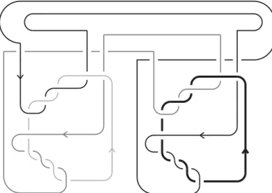
We begin by showing that three crossing changes involving justL2andL3do not suffice to split the link. We take the two-fold covering linkJ with respect toL1. The result of an isotopy to prepare for taking such a covering is shown on the right of Figure 10. The resulting covering linkJ is shown in Figure 11. The link J has splitting number 10 by Lemma 2.1, with a sharp lower bound given by the sum of the absolute values of the linking numbers between the components. By Corollary 3.6, we have that sp1(L)5.
Combining sp1(L) 5 with the linking number, it follows that if sp(L) 3, then exactly one crossing change involving (L2, L3) is required to split the link, and there can be either two additional (L1, L2) crossing changes, or two (L1, L3) crossing changes. We will give the argument to show that the first possibility cannot happen; the argument discounting the second possibility is analogous.
Suppose that two (L1, L2) crossing changes and one (L2, L3) crossing change yields the unlink. Applying Corollary 3.3 (with m= 3,α= 2, β = 1,g4(Lk) = 0), it follows that the covering link J ⊂ S3 bounds an oriented surface F of Euler characteristic 2(3−1)−2−4 =−2 that is smoothly embedded in D4 and has no closed component.
Also,F is connected by the last part of Corollary 3.3 since bothL1 andL3are involved
L2
L1
L3
Figure 10. Left: the linkL12a1622. Right: the same link, after an isotopy to prepare for taking a covering link by branching over the top component.
Figure 11. The two-fold covering link of the link in Figure 10, branched overL1.
in some crossing change withL2. SinceJ has four components,F is a three-punctured disc. That is,J is weakly slice.
To show that this cannot be the case forJ, we use the link signature invariant, which is defined similarly to the knot signature: for a linkJ, choose a surfaceV inS3bounded by J (V may be disconnected), define the Seifert pairing onH1(V) and an associated Seifert matrixAas usual. Then thelink signatureofJis defined byσ(J) = sign(A+AT). Due to Murasugi [15], if anm-component linkJ bounds a smoothly embedded oriented surface F in D4, we have |σ(J)| 2g(F) +m−b0(F), where g(F) is the genus and b0(F) is the zeroth Betti number ofF. For our covering linkJ, since it bounds a three-punctured disc in D4, we have |σ(J)| 3. Here we orient J as in Figure 11; this orientation is obtained using the orientations ofL2 and L3 shown on the right of Figure 10. On the other hand, a computation aided by aPythonsoftware package of the first author shows