Catching Growth Determinants with the Adaptive LASSO

IHS Economics Series Working Paper 232

November 2008

Catching Growth Determinants with the Adaptive LASSO

Ulrike Schneider

Martin Wagner

Impressum Author(s):

Ulrike Schneider, Martin Wagner Title:

Catching Growth Determinants with the Adaptive LASSO ISSN: Unspecified

2008 Institut für Höhere Studien - Institute for Advanced Studies (IHS) Josefstädter Straße 39, A-1080 Wien

E-Mail: o ce@ihs.ac.atffi Web: ww w .ihs.ac. a t

All IHS Working Papers are available online: http://irihs. ihs. ac.at/view/ihs_series/

This paper is available for download without charge at:

https://irihs.ihs.ac.at/id/eprint/1878/

Catching Growth Determinants with the Adaptive LASSO

Ulrike Schneider, Martin Wagner

232

Reihe Ökonomie

Economics Series

232 Reihe Ökonomie Economics Series

Catching Growth Determinants with the Adaptive LASSO

Ulrike Schneider, Martin Wagner November 2008

Institut für Höhere Studien (IHS), Wien

Institute for Advanced Studies, Vienna

Contact:

Ulrike Schneider Department of Statistics University of Vienna Universitätsstraße 5 1010 Vienna, Austria Fax: +43/1/4277-386 59 : +43/1/4277-386 45

email: ulrike.schneider@univie.ac.at

Martin Wagner

Department of Economics and Finance Institute for Advanced Studies Stumpergasse 56

1060 Vienna, Austria Fax: +43/1/599 91-163 : +43/1/599 91-150

email: Martin.Wagner@ihs.ac.at

Founded in 1963 by two prominent Austrians living in exile – the sociologist Paul F. Lazarsfeld and the economist Oskar Morgenstern – with the financial support from the Ford Foundation, the Austrian Federal Ministry of Education and the City of Vienna, the Institute for Advanced Studies (IHS) is the first institution for postgraduate education and research in economics and the social sciences in Austria.

The Economics Series presents research done at the Department of Economics and Finance and aims to share “work in progress” in a timely way before formal publication. As usual, authors bear full responsibility for the content of their contributions.

Das Institut für Höhere Studien (IHS) wurde im Jahr 1963 von zwei prominenten Exilösterreichern – dem Soziologen Paul F. Lazarsfeld und dem Ökonomen Oskar Morgenstern – mit Hilfe der Ford- Stiftung, des Österreichischen Bundesministeriums für Unterricht und der Stadt Wien gegründet und ist somit die erste nachuniversitäre Lehr- und Forschungsstätte für die Sozial- und Wirtschafts- wissenschaften in Österreich. Die Reihe Ökonomie bietet Einblick in die Forschungsarbeit der Abteilung für Ökonomie und Finanzwirtschaft und verfolgt das Ziel, abteilungsinterne Diskussionsbeiträge einer breiteren fachinternen Öffentlichkeit zugänglich zu machen. Die inhaltliche Verantwortung für die veröffentlichten Beiträge liegt bei den Autoren und Autorinnen.

Abstract

This paper uses the adaptive LASSO estimator to determine the variables important for economic growth. The adaptive LASSO estimator is a computationally very simple procedure that performs at the same time both consistent parameter estimation and model selection.

The methodology is applied to three data sets, the data used in Sala-i-Martin et al. (2004), in Fernandez et al. (2001) and a data set for the regions in the European Union. The results for the former two data sets are very similar in many respects to those found in the published papers, yet are obtained at a tiny fraction of computational cost. Furthermore, the results for the regional data highlight the importance of human capital for economic growth.

Keywords

Adaptive LASSO, economic convergence, growth regressions, model selection

JEL Classification

C31, C52, O11, O18, O47

Comments

Financial support from the Jubiläumsfonds of the Oesterreichische Nationalbank (Project number:

11688) and the European Commission's DG REGIO within the study "Analysis of the Main Factors of Regional Growth: An in-depth study of the best and worst performing European regions" is gratefully acknowledged. The regional data set has been compiled and made available to us by Robert Stehrer from the Vienna Institute for International Economic Studies (WIIW). The comments of participants of a workshop held at WIIW and of seminar participants at Universitat Pompeu Fabra, Barcelona, are gratefully acknowledged. The usual disclaimer applies.

Contents

1 Introduction 1

2 The LASSO and Adaptive LASSO Estimators 3

3 Empirical Analysis 7

3.1 Sala-i-Martin, Doppelhofer and Miller Data ... 7 3.2 Fernandez, Ley and Steel Data ... 11 3.3 European Regional Data ... 12

4 Summary and Conclusions 16

References 17 Appendix A: Description of Regional Data Set 20

Appendix B: Additional Empirical Results 23

1 Introduction

The econometric analysis of economic growth and potential economic convergence of per capita GDP has been a major research topic in the last decades. This highly active field has been revived amongst others by the influential contributions of Baumol (1986), Barro (1991) and Barro and Sala-i-Martin (1992). Numerous different econometric approaches and techniques have been employed as surveyed by Durlauf et al. (2005). Yet, few definite results have emerged, in the words of Durlauf et al. (2005, p. 558):

“The empirical study of economic growth occupies a position that is notably uneasy. Un- derstanding the wealth of nations is one of the oldest and most important research agendas in the entire discipline. At the same time, it is also one of the areas in which genuine progress seems hardest to achieve. The contributions of individual papers can often appear slender.

Even when the study of growth is viewed in terms of a collective endeavor, the various papers cannot easily be distilled into a consensus that would meet standards of evidence routinely applied in other fields of economics.”

The largest part of the empirical studies undertaken deals with so-called growth (or Barro) regressions, in which the average growth rate of per capita GDP is regressed on initial per capita GDP and a potentially large set of other explanatory variables. Such equations have their original motivation in first order approximations (around the steady state) of the Solow- Swan or Ramsey-Cass-Koopmans versions of the one-sector growth model, as illustrated in Barro (1991) or Mankiw et al. (1992). Based on these approximations numerous researchers have estimated vast amounts of equations including a large variety of additional explanatory variables. Due to the relatively weak link between the specified equations and growth theory such empirical studies have to be seen to a certain extent as data mining exercises.

Given the data mining character of growth regressions many empirical strategies have been followed to separate the wheat from the chaff. Sala-i-Martin (1997b) runs two million regressions and uses a modification of the extreme bounds test of Leamer (1985), used in the growth context earlier also by Levine and Renelt (1992), to single out what he calls

‘significant’ variables. Fernandez et al. (2001) and Sala-i-Martin et al. (2004) use Bayesian model averaging techniques to identify important growth determinants. Doing so necessitates the estimation of a large number of potentially ill-behaved regressions (e.g. in case of near multi-collinearity of the potentially many included regressors). Hendry and Krolzig (2004)

1

use, similar to Hoover and Perez (2004), a general-to-specific modelling strategy to cope with the large amount of regressors whilst avoiding the estimation of large numbers of equations.

Clearly, also in a general-to-specific analysis a certain number, typically greater than one, of regressions has to be estimated.

In this paper we determine the variables important for economic growth by resorting to recently developed statistical techniques designed to achieve at the same time consistent pa- rameter estimation and model selection. In particular we use the so-called adaptive LASSO (Least Absolute Shrinkage and Selection Operator) estimator, a variant of the LASSO esti- mator (Tibshirani, 1996), proposed by Zou (2006) and briefly described in Section 2. This approach has several advantages. First, it is computationally very cheap, e.g. when using the algorithm proposed by Efron et al. (2004) the whole sequence (see Section 2) of regressions estimated has roughly the same computational cost as one single OLS regression including all regressors. Second, the step-wise forward selection nature of the procedure with the optimal termination (see the discussion in Section 2) determined either by minimizing an information criterion or by cross-validation typically avoids using results based on ill-behaved regressions.

This is most likely an advantage compared to general-to-specific approaches in case that re- gressions including many variables are ill-behaved or cannot even be estimated by OLS (e.g.

in case there are more explanatory variables than observations). Third, the estimator can be tuned (see Section 2) to perform consistent model selection. Within the growth context this means a consistent decision concerning which variables are related to growth and which are not. Finally, for those who prefer to use classical statistical methods over Bayesian methods and estimates based on a single model over averages, the adaptive LASSO provides exactly that.

We apply the method to several data sets, with two of them taken from widely cited papers.

The first data set is the one used in Sala-i-Martin et al. (2004), containing 67 explanatory variables for 88 countries. The second one is the Fernandez et al. (2001) data set, based in turn on data used in Sala-i-Martin (1997b), which contains 41 explanatory variables for 72 countries. The third data set we use comprises the 255 European NUTS2 regions in the 27 member states of the European union and contains 48 explanatory variables. The results for the first two data sets are in several respects similar to the findings in the original papers.

For both data sets the adaptive LASSO estimator selects slightly less than 15 explanatory variables, with about 10 of them coinciding with the most important ones of the original

2

papers (as measured there by the posterior inclusion probabilities). All coefficient estimates have the expected signs and plausible values. The results for the regional data, for which fewer core economic data are available as explanatory variables, indicate the importance of human capital, proxied by medium and high education, for economic growth.

The paper is organized as follows. In Section 2 we describe the statistical methods applied.

Section 3 contains the empirical analysis and results and Section 4 briefly summarizes and concludes. Two appendices follow the main text. Appendix A briefly describes the regional data and Appendix B collects some additional empirical results.

2 The LASSO and Adaptive LASSO Estimators

The LASSO estimator and its variant, the adaptive LASSO estimator are special cases of the general class of penalized least squares (PLS) estimators . For a linear regression model y = Xβ + ε (y, ε ∈ R

, X ∈ R

), a PLS estimator ˆ β of β is in this paper defined as the solution of the minimization problem

β∈

min

ky − Xβk

+ λ

pen(β), (1)

where λ

is the so-called tuning parameter and pen(β) the penalty function. Clearly, dif- ferent penalty terms give rise to different estimators. The general class of Bridge estimators was introduced by Frank and Friedman (1993) and refers to estimators defined by (1) with pen(β) = P

j=1

|β

|

. Note that γ = 2 corresponds to the well-known Ridge estimator. For γ ≤ 1, due to the structure of the underlying optimization problem, coordinates of the es- timated coefficient vector ˆ β can (potentially) be exactly equal to zero and in that sense the resulting estimator can be viewed to perform also model selection. The case γ = 1 corre- sponds to the LASSO estimator, which was separately treated in Tibshirani (1996) who also introduced the name for this estimator. By definition in case γ = 1 the penalty function is given by the l

-norm of the coefficient vector.

Given standard assumptions on the regression model described below, the asymptotic properties of the LASSO estimator (and PLS estimators in general) largely depend on the asymptotic choice of the tuning parameter λ

, as studied in Knight and Fu (2000) for Bridge estimators. For the LASSO, estimation consistency always holds if λ

/ √

N tends to zero as N tends to infinity. Given this basic condition on the tuning parameter, two different asymptotic regimes are of interest. The LASSO estimator might either be tuned consistently

3

or conservatively, that is, the estimator either performs consistent model selection (finding the correct zero coefficients with asymptotic probability equal to one) if λ

tends to infinity or it carries out conservative model selection (recovering the correct zero coefficients with asymptotic probability less than one) if λ

converges to a finite number. If consistent model selection is the asymptotic regime of choice, it turns out that for the LASSO additional conditions on the regressors are necessary. Such conditions are treated, for instance, in Meinshausen and B¨ uhlmann (2006) and Zhao and Yu (2006).

For the adaptive LASSO estimator as introduced in Zou (2006), consistent tuning is always possible for linear regression models under standard assumptions. As mentioned before, the adaptive LASSO estimator, ˆ β

, is a variant of the LASSO estimator with a randomly weighted l

-penalty function. More concretely, it is defined as the solution of the minimization problem

min

β∈R^k

ky − Xβk

+ λ

X

j=1

|β

|/| β ˜

|, (2) where ˜ β is any √

N -consistent initial estimator of β, for instance the OLS estimator, if avail- able. The idea is to put a larger penalty on “seemingly small” coefficients to enhance robust- ness. The pointwise asymptotic properties of ˆ β

in the consistently tuned case have been derived in Theorem 2 in Zou (2006) and are summarized in the following proposition. Consider a linear regression setting with dependent variable y = (y

, . . . , y

)

, per capita GDP growth in our context, regressors x

= (x

, . . . , x

)

for j = 1, . . . , k, written as X = [x

, . . . , x

] in matrix format. Assume the relation y

= x

β

+ ε

holds for some β

∈ R

, the true param- eter, with ε

i.i.d. with mean 0 and variance σ

for i = 1, . . . , N. Moreover, we assume that X

X/N → C as N → ∞ for some positive definite matrix C. Denote by A = {j : β

6= 0}

the index set of the unknown true non-zero coefficients and by β

the vector of length |A|

restricted to that index set. Under these assumptions the following result holds.

Proposition 1 (Zou, 2006) Suppose that λ

/ √

N → 0 and λ

→ ∞. Then β ˆ

performs consistent model selection and

√

N ( ˆ β

− β

) −→

N (0, Σ

), (3)

where Σ

refers to the asymptotic covariance matrix of the (infeasible) OLS estimator under the unknown true zero restrictions.

4

Note that the asymptotic behavior of ˆ β

as described in Proposition 1 is sometimes referred to as the oracle property, a term introduced in Fan and Li (2001). The distributional result in (3) appears to suggest that the adaptive LASSO estimator performs as well as the OLS estimator for the unknown correct model, i.e. as if the true restrictions were known.

This explains the name oracle property. However, Leeb and P¨ otscher (2008) and P¨ otscher and Schneider (2008) show in detail that these pointwise asymptotic properties need to be interpreted with great care. Amongst other issues in relation to estimator risk it can in particular be shown that consistent model selection has detrimental impacts on the length of so-called “honest” confidence intervals, which become necessarily much larger than those for unpenalized least squares estimators or conservative model selection procedures (see P¨ otscher, 2007).

We now discuss computational issues of the adaptive LASSO estimator. Solutions to the minimization problem in (2) can be computed very efficiently exploiting the specific structure of the problem. It can be shown that the solutions to the corresponding optimization problems are piecewise linear in the tuning parameter λ

, see e.g. Rosset and Zhu (2007). Exploiting this property, the estimator can easily be computed for all tuning parameters λ

∈ [0, ∞), leading to so-called solution paths for each variable. These solution paths are initiated at λ

equal to infinity where all coefficients are equal to zero and ensued to λ

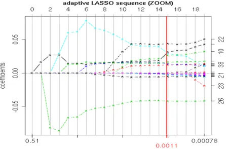
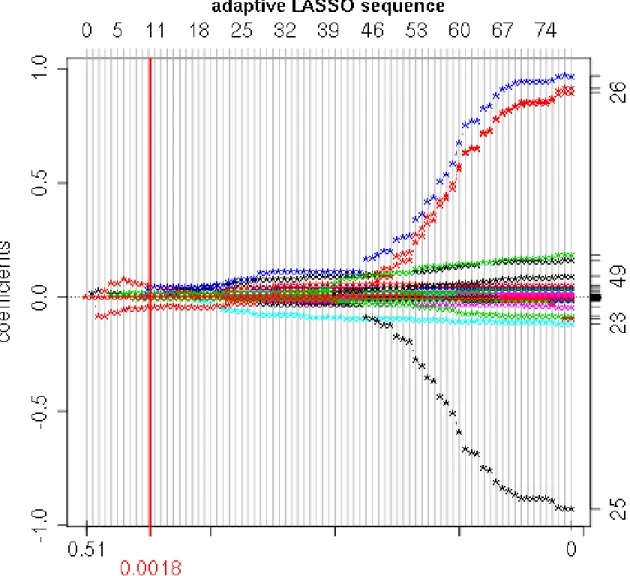
equal to zero corresponding to the OLS estimator (in case it is uniquely defined). In each step along this sequence, one variable is either included or removed from the current “active” subset, i.e. the set containing the coefficients that are not equal to zero in that step, as illustrated in Figure 1 and Figure 2 in Appendix B for the Sala-i-Martin et al. (2004) data set. These figures should be read as follows. On the horizontal axis the steps of the sequence are plotted equidistantly, e.g. in Figure 1 the first twenty steps are plotted and in between each of these steps the estimated coefficients are linear in λ

. This implies that the scaling of the horizontal axis is in general not linear with respect to the tuning parameter λ

. In the example the value of the tuning parameter at which the first estimated coefficient starts to become non-zero is λ

= 0.51. The numbers on the right hand side of the graph indicate the variable number, e.g. the index 26 refers to the share of expenditure of government consumption of GDP in 1961 (for the variable abbreviations and their numbers for the Sala-i-Martin et al. (2004) data see Table 1). The corresponding line plots the coefficient corresponding to this variable as a function of the tuning parameter. The vertical line at λ

= 0.0011 indicates the optimal

5

Figure 1: Zoom of Figure 2: Coefficient paths of adaptive LASSO estimation for the Sala-i- Martin et al. (2004) data set for the first 20 steps of the adaptive LASSO estimation sequence.

The vertical line at λ

= 0.00111 indicates the optimal tuning parameter λ

chosen by cross- validation.

choice of the tuning parameter according to cross-validation, see below.

To provide a “final” subset of variables together with a corresponding estimate of the parameter vector different approaches are used to choose the tuning parameter. One of them is given by minimizing a BIC-type information criterion, see e.g. Wang and Leng (2007). Doing so can be shown to result in consistent model selection. Another widely- used procedure is given by (k-fold) cross-validation, see e.g. Leng et al. (2006). This latter procedure may result in conservative model selection, i.e. it may lead to the inclusion of some variables whose true coefficients are equal to zero. The results reported in this paper are based on cross-validation, given the results obtained with this approach in a variety of experiments. Since cross-validation is potentially conservative the resultant estimates are not prone to amongst others the problems of confidence sets based on consistent tuning, as briefly mentioned above (compare again P¨ otscher, 2007). In our applications rather small models are chosen by cross-validation so that we do not see the potential conservativeness as a major concern with respect to the inclusion of irrelevant variables.

6

3 Empirical Analysis

As mentioned in the introduction, the empirical analysis is performed for three different data sets. These are the data sets used in Sala-i-Martin et al. (2004), in Fernandez et al. (2001) and a data set covering the 255 NUTS2 regions of the European Union. In the discussion below we retain the variable names from the data files we received from Gernot Doppelhofer for the Sala-i-Martin et al. (2004) data and also use the original names used in the file downloaded from the homepage of the Journal of Applied Econometrics for the Fernandez et al. (2001) data to facilitate the comparison with the results in these papers.

3.1 Sala-i-Martin, Doppelhofer and Miller Data

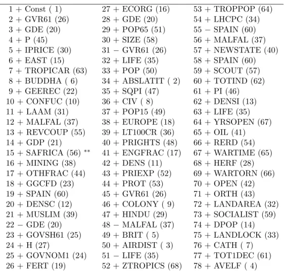
The data set considered in Sala-i-Martin et al. (2004) contains 67 explanatory variables for 88 countries. The variables and their sources are described in detail in Table 1 in Sala-i- Martin et al. (2004, p. 820–821). The dependent variable is the average annual growth rate of real per capita GDP over the period 1960–1996. In Table 1 we present the sequence of adaptive LASSO moves (i.e. the sequence of variables in- respectively excluded from the set of active variables as λ

→ 0) for this data set. As already discussed in the previous section, graphical information concerning the whole sequence of estimated coefficients as a function of the tuning parameter λ

is presented in Figure 2 in Appendix B.

The full regressor matrix comprising the constant and all 67 explanatory variables is almost multi-collinear, with a reciprocal condition number of 9.38 × 10

. The full OLS estimator is thus very imprecisely defined at best. To be precise, in order to invert the X

X matrix the numerical tolerance has to be set to an extremely small number. To avoid using the ill-defined OLS estimator we acknowledge the (numerical) multi-collinearity in the regressor matrix and use as initial estimator the (standard) LASSO estimator at the end of the solution path, i.e. for λ

= 0. This corresponds to the solution of the normal equations with the smallest l

-norm, due to continuity of the coefficient paths in the tuning parameter. One could also use different regularized initial estimators, e.g. the Ridge estimator, for which, however, a choice concerning the Ridge parameter has to be made. Note that for the two other data sets considered we use the OLS estimator as initial estimator since for those no multi-collinearity problems arise.

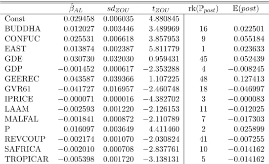
Choosing the tuning parameter by cross-validation leads to a model with 15 regressors including the constant. The estimation results are presented in Table 2. The following 14

7

1 + Const ( 1) 27 + ECORG (16) 53 + TROPPOP (64)

2 + GVR61 (26) 28 + GDE (20) 54 + LHCPC (34)

3 + GDE (20) 29 + POP65 (51) 55 − SPAIN (60)

4 + P (45) 30 + SIZE (58) 56 + MALFAL (37)

5 + IPRICE (30) 31 − GVR61 (26) 57 + NEWSTATE (40)

6 + EAST (15) 32 + LIFE (35) 58 + SPAIN (60)

7 + TROPICAR (63) 33 + POP (50) 59 + SCOUT (57) 8 + BUDDHA ( 6) 34 + ABSLATIT ( 2) 60 + TOTIND (62) 9 + GEEREC (22) 35 + SQPI (47) 61 + PI (46) 10 + CONFUC (10) 36 + CIV ( 8) 62 + DENSI (13) 11 + LAAM (31) 37 + POP15 (49) 63 + LIFE (35) 12 + MALFAL (37) 38 + EUROPE (18) 64 + YRSOPEN (67) 13 + REVCOUP (55) 39 + LT100CR (36) 65 + OIL (41)

14 + GDP (21) 40 + PRIGHTS (48) 66 + RERD (54) 15 + SAFRICA (56)

41 + ENGFRAC (17) 67 + WARTIME (65) 16 + MINING (38) 42 + DENS (11) 68 + HERF (28) 17 + OTHFRAC (44) 43 + PRIEXP (52) 69 + WARTORN (66) 18 + GGCFD (23) 44 + PROT (53) 70 + OPEN (42) 19 + SPAIN (60) 45 + GVR61 (26) 71 + ORTH (43) 20 + DENSC (12) 46 + COLONY ( 9) 72 + LANDAREA (32) 21 + MUSLIM (39) 47 + HINDU (29) 73 + SOCIALIST (59) 22 − GDE (20) 48 − MALFAL (37) 74 + DPOP (14) 23 + GOVSH61 (25) 49 + BRIT ( 5) 75 + LANDLOCK (33)

24 + H (27) 50 + AIRDIST ( 3) 76 + CATH ( 7)

25 + GOVNOM1 (24) 51 − LIFE (35) 77 + TOT1DEC (61) 26 + FERT (19) 52 + ZTROPICS (68) 78 + AVELF ( 4)

Table 1: Sequence of adaptive LASSO moves for the Sala-i-Martin et al. (2004) data. The entries in the table read as follows. The integers enumerate the step, + indicates inclusion of a variable in this step, whereas − indicates exclusion of a variable. The included/excluded variable is the third element of each entry and the numbers in brackets refer to the number of the variable in the data base. The superscript

indicates the set of active variables based on cross-validation, i.e. the variables included in the active set up to this step.

8

β ˆ

sd

t

rk( P

) E (post)

Const 0.029458 0.006035 4.880845

BUDDHA 0.012027 0.003446 3.489969 16 0.022501

CONFUC 0.025531 0.006618 3.857953 9 0.055184

EAST 0.013874 0.002387 5.811779 1 0.023633

GDE 0.030730 0.032030 0.959431 45 0.052439

GDP −0.001452 0.000617 −2.353288 4 −0.008245

GEEREC 0.043587 0.039366 1.107225 48 0.127413

GVR61 −0.041727 0.016957 −2.460748 18 −0.046997

IPRICE −0.000071 0.000016 −4.382702 3 −0.000083

LAAM −0.002593 0.001220 −2.126153 11 −0.012025

MALFAL −0.001841 0.000872 −2.110789 7 −0.017303

P 0.016097 0.003649 4.411460 2 0.025899

REVCOUP −0.002174 0.001070 −2.030824 41 −0.007255 SAFRICA −0.002010 0.000708 −2.837761 10 −0.014162 TROPICAR −0.005398 0.001720 −3.138131 5 −0.014162

Table 2: Estimation results for the Sala-i-Martin et al. (2004) data. The first three result columns correspond to the adaptive LASSO estimates, with the standard errors and t-values computed as described in Zou (2006). The column labelled rk(P

) reports the ranks accord- ing to posterior inclusion probabilities from Sala-i-Martin et al. (2004, Table 3, p. 828–829) and the column labelled E (post) reports the posterior means from Sala-i-Martin et al. (2004, Table 4, p. 830).

variables are important to explain cross-country growth, listed in alphabetical order of vari- able abbreviation, where we also show the sign of the corresponding coefficient in parenthesis:

BUDDHA (fraction of population Buddhist in 1960, positive), CONFUC (fraction of popula- tion Confucian in 1960, positive), EAST (East Asian dummy, positive), GDE (average share of public expenditure on defense, positive), GDP (log per capita GDP in 1960, negative), GEEREC (average share of public expenditure on education, positive), GVR61 (share of ex- penditure on government consumption of GDP in 1961, negative), IPRICE (investment price, negative), LAAM (Latin American dummy, negative), MALFAL (index of malaria prevalence in 1966, negative), P (primary school enrollment rate, positive), REVCOUP (number of revo- lutions and coups, negative), SAFRICA (sub-Saharan Africa dummy, negative), TROPICAR (fraction of country’s land in tropical area, negative). The coefficient signs are all as expected and also the magnitude of the coefficients is plausible and not out of line from other findings in the literature, see also below.

With two exceptions the coefficients are statistically different from zero, with the standard errors computed according to Zou (2006) based on Tibshirani (1996). The two variables

9

with insignificant coefficients are both related to government expenditures. These are the average share of public expenditure on defense and the average share of public expenditure on education. Out of the government expenditure related variables only the government consumption share of GDP appears to be significant with a negative impact on growth. The negative coefficient sign is in line with a stylized relationship in public finance referred to as Wagner’s law (formulated by the German economist Adolph Wagner in the nineteenth century), which states that richer countries have a higher public expenditure share. Thus, in case of convergence, in which richer countries grow slower, this is consistent with a negative coefficient of the government consumption share of GDP. However, like many empirical growth studies we do not find strong evidence for government expenditure related variables to be major determinants of economic growth. Here we find three government expenditure variables, but two of them with coefficients that are not significantly different from zero.

The fourth results column in Table 2 displays the ranks according to the posterior inclusion probabilities as given in Sala-i-Martin et al. (2004, Table 3, p. 828–829). There is a substantial degree of similarity of our results to theirs in that we find 8 of their top 10 variables (and 9 of their top 14 variables). Of the top 14 variables of Sala-i-Martin et al. (2004) we do not find the following. Population density in coastal areas in the 1960s (DENSC), life expectancy in 1960 (LIFEEXP), fraction of GDP in mining (MINING), the dummy for being a Spanish colony (SPAIN) and the number of years open (YRSOPEN). Our results suggest instead the importance of the following variables (where we only report the statistically significant variables, which excludes the two mentioned government expenditure variables). The fraction of Buddhists in the population, the number of revolutions and coups and the government consumption share of GDP in the 1960s.

In the last column of Table 2 we report the posterior means of the estimated coefficients as given in Sala-i-Martin et al. (2004, Table 4, p. 830). The signs of our coefficient estimates throughout coincide with the signs of the posterior means reported in the final column. Our point estimates are typically somewhat smaller (in absolute value) than the posterior means of Sala-i-Martin et al. (2004). Notwithstanding the fact that the estimates are based on very different approaches this might be a reflection of the fact that the adaptive LASSO estimates are to a certain extent biased towards zero in finite samples due to the PLS setup.

10

3.2 Fernandez, Ley and Steel Data

The data set used by Fernandez et al. (2001) is based on the data set used in Sala-i-Martin (1997b). In particular they select a subset of the Sala-i-Martin data that contains the 25 variables singled out as important by Sala-i-Martin (1997b). These variables are available for 72 countries. To these they add 16 further variables which are also available for these 72 countries, which makes a total of 41 explanatory variables. The dependent variable is the average annual growth rate of real per capita GDP over the period 1960–1992. A detailed description of the variables and their sources is contained in the working paper Sala-i-Martin (1997a, Appendix 1).

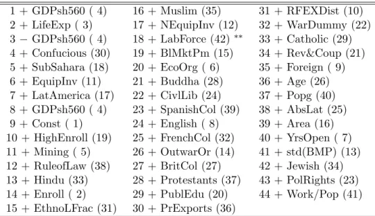
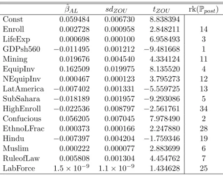
Cross-validation, see Table 3 for the sequence of variables included, leads to an equa- tion including 16 explanatory variables counting the intercept. The following variables are selected, using the ordering in the data file. Enroll (primary school enrollment in 1960, positive), LifeExp (life expectancy in 1960, positive), GDPsh560 (log of per capita GDP in 1960, negative), Mining (fraction of GDP in mining, positive), EquipInv (equipment invest- ment, positive), NEquipInv (non-equipment investment, positive), LatAmerica (dummy for Latin America, negative), SubSahara (dummy for sub-Saharan Africa, negative), HighEnroll (enrollment rates in higher education, negative), Confucius (share of population Confucian, positive), EthnoLFrac (ethnolinguistic fractionalization, positive), Hindu (share of population Hindu, negative), Muslim (share of population Muslim, positive), RuleofLaw (rule of law, pos- itive) and LabForce (size of labor force, positive). Again, negative and positive indicate the signs of the corresponding coefficients.

Our results concerning variable selection correspond to a large extent with those of Fer- nandez et al. (2001, Table I, p. 569) with respect to posterior inclusion probabilities. In particular 11 of the 15 variables included in our results are amongst the top 15 of the vari- ables of Fernandez et al. (2001). The 4 of their top 15 variables that are not included in our results are given by years of openness (YrsOpen), degree of capitalism (EcoOrg), and the fractions of Protestants (Protestants) and of Buddhists (Buddha) in the population. The 4 differing variables we obtain by applying the adaptive LASSO algorithm are the enrollment rate in higher education (HighEnroll, negative), the measure of ethnolinguistic fractionaliza- tion (EthnoLFrac, positive), the fraction of Hindus in the population (Hindu, negative) and the size of the labor force (LabForce, positive). The coefficient for the size of the labor force, meant to capture the size of the economy, is not significantly different from zero even at the

11

1 + GDPsh560 ( 4) 16 + Muslim (35) 31 + RFEXDist (10) 2 + LifeExp ( 3) 17 + NEquipInv (12) 32 + WarDummy (22) 3 − GDPsh560 ( 4) 18 + LabForce (42)

33 + Catholic (29) 4 + Confucious (30) 19 + BlMktPm (15) 34 + Rev&Coup (21) 5 + SubSahara (18) 20 + EcoOrg ( 6) 35 + Foreign ( 9) 6 + EquipInv (11) 21 + Buddha (28) 36 + Age (26) 7 + LatAmerica (17) 22 + CivlLib (24) 37 + Popg (40) 8 + GDPsh560 ( 4) 23 + SpanishCol (39) 38 + AbsLat (25) 9 + Const ( 1) 24 + English ( 8) 39 + Area (16) 10 + HighEnroll (19) 25 + FrenchCol (32) 40 + YrsOpen ( 7) 11 + Mining ( 5) 26 + OutwarOr (14) 41 + std(BMP) (13) 12 + RuleofLaw (38) 27 + BritCol (27) 42 + Jewish (34) 13 + Hindu (33) 28 + Protestants (37) 43 + PolRights (23) 14 + Enroll ( 2) 29 + PublEdu (20) 44 + Work/Pop (41) 15 + EthnoLFrac (31) 30 + PrExports (36)

Table 3: Sequence of adaptive LASSO moves for the Fernandez et al. (2001) data set. See caption to Table 1 for further explanations.

10% level. The small value for the coefficient corresponding to the size of the labor force stems from the fact that Fernandez et al. (2001) have employed persons in their data base, and not e.g. employed persons in thousands or millions. For reasons of comparability we have decided not to change the scaling of this variable. The coefficient corresponding to the fraction of Hindus is only significant at the 10% level but not at the 5% level. The negative sign of the coefficient corresponding to the high education enrollment rate may merely reflect the fact that countries with a well and broadly functioning higher education system in the 1960s have mainly been rather well developed rich countries which have subsequently grown below average.

3.3 European Regional Data

The third data set we analyze contains 48 explanatory variables for the 255 NUTS2 regions in the 27 member states of the European Union. The data and variables are described in Appendix A. The dependent variable is the average annual growth rate of per capita GDP over the period 1995–2005. On a regional level it is more difficult to obtain core economic data, hence many of the variables listed in Table 8 in Appendix A are related to infrastructure characteristics (meant in very broad sense also including dummy variables whether the regions are located on the seaside or at country borders) and labor market

12

β ˆ

sd

t

rk( P

)

Const 0.059484 0.006730 8.838394

Enroll 0.002728 0.000958 2.848211 14

LifeExp 0.000698 0.000100 6.958493 3

GDPsh560 −0.011495 0.001212 −9.481668 1

Mining 0.019676 0.004540 4.334124 11

EquipInv 0.162509 0.019975 8.135520 4

NEquipInv 0.000467 0.000123 3.795273 12 LatAmerica −0.007402 0.001331 −5.559725 13 SubSahara −0.018189 0.001957 −9.293086 5 HighEnroll −0.022536 0.008797 −2.561761 34 Confucious 0.056205 0.007045 7.978490 2 EthnoLFrac 0.000373 0.000166 2.247880 28

Hindu −0.007397 0.004204 −1.759346 19

Muslim 0.000222 0.000077 2.883699 6

RuleofLaw 0.005808 0.001304 4.454762 7 LabForce 1.5 × 10

1.1 × 10

1.434628 25

Table 4: Estimation results for the Fernandez et al. (2001) data. The final column reports the rank according to posterior inclusion probabilities from Fernandez et al. (2001, Table I, p. 569). See caption to Table 2 for further explanations.

variables (unemployment and activity rates, as well as some broad education characteristics in the working age population).

Given that there are both large intra- and inter-country differences in the economic perfor- mance of the European regions our preferred set of variables to perform the adaptive LASSO estimation sequence contains country dummies for the 19 out of the 27 countries that consist of more than just one region. Taking into account the divide in formerly centrally planned economies we also consider a specification with a dummy for all Central and Eastern Euro- pean (CEE) countries. For completeness we also consider a specification without any country dummy variables.

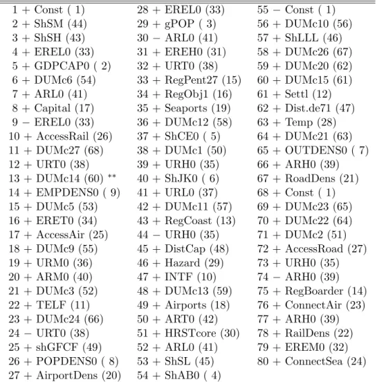
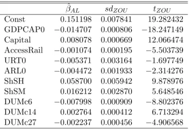
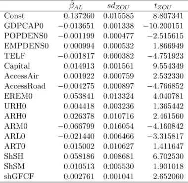
For the setup with 19 country dummies cross-validation leads to termination of the es- timation sequence at step 13, leading to an equation including 11 regressors including the intercept, see Tables 5 and 6. The included explanatory variables and the coefficient signs are: GDPCAP0 (log of per capita GDP in 1995, negative), Capital (dummy for capital city, positive), AccessRail (measure of accessibility by railroad, negative), URT0 (unemployment rate total in 1995, negative), ARL0 (activity rate of low educated in 1995, negative), ShSH (share of high educated in labor force, positive), ShSM (share of medium educated in labor

13

1 + Const ( 1) 28 + EREL0 (33) 55 − Const ( 1) 2 + ShSM (44) 29 + gPOP ( 3) 56 + DUMc10 (56) 3 + ShSH (43) 30 − ARL0 (41) 57 + ShLLL (46) 4 + EREL0 (33) 31 + EREH0 (31) 58 + DUMc26 (67) 5 + GDPCAP0 ( 2) 32 + URT0 (38) 59 + DUMc20 (62) 6 + DUMc6 (54) 33 + RegPent27 (15) 60 + DUMc15 (61) 7 + ARL0 (41) 34 + RegObj1 (16) 61 + Settl (12) 8 + Capital (17) 35 + Seaports (19) 62 + Dist.de71 (47) 9 − EREL0 (33) 36 + DUMc12 (58) 63 + Temp (28) 10 + AccessRail (26) 37 + ShCE0 ( 5) 64 + DUMc21 (63) 11 + DUMc27 (68) 38 + DUMc1 (50) 65 + OUTDENS0 ( 7) 12 + URT0 (38) 39 + URH0 (35) 66 + ARH0 (39) 13 + DUMc14 (60)

40 + ShJK0 ( 6) 67 + RoadDens (21) 14 + EMPDENS0 ( 9) 41 + URL0 (37) 68 + Const ( 1) 15 + DUMc5 (53) 42 + DUMc11 (57) 69 + DUMc23 (65) 16 + ERET0 (34) 43 + RegCoast (13) 70 + DUMc22 (64) 17 + AccessAir (25) 44 − URH0 (35) 71 + DUMc2 (51) 18 + DUMc9 (55) 45 + DistCap (48) 72 + AccessRoad (27) 19 + URM0 (36) 46 + Hazard (29) 73 + URH0 (35) 20 + ARM0 (40) 47 + INTF (10) 74 − ARH0 (39) 21 + DUMc3 (52) 48 + DUMc13 (59) 75 + RegBoarder (14) 22 + TELF (11) 49 + Airports (18) 76 + ConnectAir (23) 23 + DUMc24 (66) 50 + ART0 (42) 77 + ARH0 (39) 24 − URT0 (38) 51 + HRSTcore (30) 78 + RailDens (22) 25 + shGFCF (49) 52 + ARL0 (41) 79 + EREM0 (32) 26 + POPDENS0 ( 8) 53 + ShSL (45) 80 + ConnectSea (24) 27 + AirportDens (20) 54 + ShAB0 ( 4)

Table 5: Sequence of adaptive LASSO moves for the regional data set including country dummies for all countries consisting of more than one region. See caption to Table 2 for further explanations.

14

force, positive), DUMc6 (dummy for Germany, negative), DUMc14 (dummy for Ireland, pos- itive) and DUMc27 (dummy for UK, negative). The signs of the coefficients are with the exception of AccessRail in line with expectations. With respect to rail accessibility it has to be noted that European railroad infrastructure has been built to a very large degree before the sample period of 1995–2005. In particular a large number of the regions that are most well accessible by railroads have experienced fast growth and development in much earlier periods than over the last decade and are now slower growing regions with high development levels. Some well-connected regions hosting from today’s perspective “old industries”, as e.g.

the German Ruhr area, even experience difficulties in the industrial restructuring process.

These two observations explain the negative coefficient for AccessRail. Clearly, this example again highlights the need for careful interpretation of regression results.

The set of human capital and labor market variables included in the specified equation hints at the importance of a well-educated labor force for economic growth.

Of course, a large share of high educated people in the labor force requires as a complement the presence of a sufficient number of workplaces where these skills are required, i.e. sufficiently many compa- nies offering a sufficiently high number of jobs requiring medium or high skills and education.

Also the negative coefficient for the activity rate of low educated has to be interpreted in the same way, i.e. taking into account that complementarity with typically low value added creating activities. Due to the relatively short time span of only 10 years using initial values of the explanatory variables may not completely resolve these potential endogeneity issues.

It is worth noting that only three country dummies appear to have explanatory power:

these cover the poor growth performers Germany and the UK and the “Celtic tiger” Ireland.

The findings are quite robust when compared to findings obtained without country dummies or when including only the CEE dummy. For details see Tables 9 to 12 in Appendix B.

Excluding country dummies leads to the inclusion of some additional variables, in partic- ular initial population density (negative) and employment density (positive) as well as the initial share of gross fixed capital formation in gross value added (positive). AccessRail is substituted by AccessAir (positive) and AccessRoad (negative). Note also that, as expected, the number of variables included is larger when no country dummies are considered. Includ-

1It is important to note here again that the available data mainly allow to capture the influence of human capital. There are no variables that measure or at least proxy physical capital and also proxies for technology are essentially absent. The only exception is the share of gross fixed capital formation in gross value added in the initial period. Scarcity of data clearly limits any quantitative study of regional growth.

15

β ˆ

sd

t

Const 0.151198 0.007841 19.282432 GDPCAP0 −0.014707 0.000806 −18.247149 Capital 0.008078 0.000669 12.066474 AccessRail −0.001074 0.000195 −5.503739 URT0 −0.005371 0.003164 −1.697749 ARL0 −0.004472 0.001933 −2.314276

ShSH 0.058700 0.005942 9.878976

ShSM 0.016212 0.002870 5.648546

DUMc6 −0.007998 0.000909 −8.802376 DUMc14 0.002764 0.000412 6.713294 DUMc27 −0.002237 0.000456 −4.906568

Table 6: Estimation results for the regional data set including country dummies for all coun- tries consisting of more than one region. See caption to Table 2 for further explanations.

ing only the dummy for the CEE countries leads to quite similar results both in terms of variables included and coefficient signs. Finally, when including distance weighted variables, the distance weighted initial output and the employment density in the initial period enter negatively with again the rest of the variables being roughly the same. Details for the results with distance weighted variables are available upon request.

4 Summary and Conclusions

In this paper we propose to use the adaptive LASSO estimator to determine the variables relevant for explaining economic growth. The adaptive LASSO estimation sequence has es- sentially the same computational cost as a single OLS regression and simultaneously performs model selection and consistent parameter estimation. Given the large uncertainty concerning potential growth determinants, reflected in large sets of explanatory variables, a consistent or conservative forward selection procedure avoiding the estimation of potentially ill-behaved regressions including large numbers of variables appears to be particularly useful. The pro- posed classical methodology avoids both the estimation and averaging of large numbers of models using (either a classical or) a Bayesian framework and also avoids the pitfalls related to inference in general-to-specific model selection procedures.

The proposed methodology is implemented for three data sets, namely the data used in

2For classical model averaging and subsequent inference in the context of growth regressions see Wagner and Hlouskova (2008).

16

Sala-i-Martin et al. (2004), in Fernandez et al. (2001) and a data set covering the regions of the European Union member states. The results for the former two well-studied data sets are quite in line with the findings in the original papers, at a tiny fraction of computational costs.

For the Sala-i-Martin et al. (2004) data set we find 12 significant explanatory variables (in an equation comprising 14 explanatory variables) using the t-values according to Zou (2006).

9 of these 12 variables are among the top 14 variables with respect to posterior inclusion probability as given in Sala-i-Martin et al. (2004). The findings for the Fernandez et al. (2001) data set also exhibit a high degree of similarity with the findings in the original paper. Here we find 15 explanatory variables, with one of them (size of the labor force) not significant at the 5% level. The set of selected variables contains 11 of the top 14 variables, again according to posterior inclusion probability, of Fernandez et al. (2001). For both data sets the sets of variables excluded with our approach compared to the findings in the original papers as well as the sets of included significant explanatory variables not found to be important in the original papers are plausible. Furthermore, also the findings obtained for the regional data set (for which only a small number of core economic variables is available) are plausible. This data set comprises many infrastructure and labor market variables and the results indicate that a well educated labor force is beneficial for economic growth.

The findings in this paper strongly indicate that the adaptive LASSO estimator may indeed be an estimation and model selection procedure that can be fruitfully employed in the growth regressions context.

References

Barro, R.J. (1991). Economic growth in a cross-section of countries. Quarterly Journal of Economics 106, 407–445.

Barro, R.J. and Sala-i-Martin, X. (1992). Convergence. Journal of Political Economy 100, 223–251.

Baumol, W.J. (1986). Productivity growth, convergence and welfare: What the long run data show. American Economic Review 76, 1072–1085.

Durlauf, S.N., Johnson, P.A. and Temple, J.R.W. (2005). Growth econometrics. In Aghion, P. and Durlauf, S.N. (eds.) Handbook of Economic Growth, Vol. 1A, Ch.8. Elsevier.

17

Efron, B., Hastie, T., Johnstone, I. and Tibshirani, R. (2004). Least angle regression. Annals of Statistics 32, 407–499.

Fan, J. and Li, R. (2001). Variable selection via nonconcave penalized likelihood and its oracle properties. Journal of the American Statistical Association, 96, 1348–1360.

Fernandez, C., Ley, E. and Steel, M.F.J. (2001). Model uncertainty in cross-country growth regressions. Journal of Applied Econometrics 16, 563–576.

Frank, I. E. and Friedman, J. H. (1993). A statistical view of some chemometrics regression tools (with discussion). Technometrics 35, 109–148.

Hendry, D.F. and Krolzig, H.-M. (2004). We ran one regression. Oxford Bulletin of Economics and Statistics 66, 799–810.

Hoover, K.D. and Perez, S.J. (2004). Truth and robustness in cross-country growth regres- sions. Oxford Bulletin of Economics and Statistics 66, 765–798.

Knight, K. and Fu, W. (2000). Asymptotics of LASSO-type estimators, Annals of Statistics 28, 1356–1378.

Leamer, E. E. (1985). Sensitivity analyses would help. American Economic Review 57, 308–

313.

Leeb, H. and P¨ otscher, B. M. (2008). Sparse estimators and the oracle property, or the return of Hodges’ estimator. Journal of Econometrics 142, 201–211.

Leng, C., Lin, Y. and Wahba G. (2006). A note on the LASSO and related procedures in model selection. Statistica Sinica 16, 1273–1284.

Levine, R. and Renelt, D. (1992). Sensitivity analysis of cross-country growth regressions.

American Economic Review 82, 942–963.

Mankiw, N.G., Romer, D., and Weil, D.N. (1992). A contribution to the empirics of economic growth. Quarterly Journal of Economics 107, 407–437.

Meinshausen, N. and B¨ uhlmann, P. (2006). Consistent neighborhood selection for high- dimensional graphs with the LASSO. Annals of Statistics 34, 1436–1462.

18

P¨ otscher, B. M. (2007). Confidence sets based on sparse estimators are necessarily large.

Manuscript arXiv:0711.1036.

P¨ otscher, B. M. and Schneider, U. (2008). On the distribution of the adaptive LASSO esti- mator. Manuscript arXiv:0801.4627.

Rosset, S. and Zhu, J. (2007). Piecewise linear regularized solution paths, Annals of Statistics 35, 1012–1030.

Sala-i-Martin, X. (1997a). I just ran 4 million regressions. NBER Working Paper No. 6252.

Sala-i-Martin, X. (1997b). I just ran 2 million regressions. American Economic Review 87, 178–183.

Sala-i-Martin, X., Doppelhofer, G. and Miller, R.I. (2004). Determinants of long-term growth:

A Bayesian averaging of classical estimates (BACE) approach. American Economic Re- view 94, 813–835.

Tibshirani, R. (1996). Regression shrinkage and selection via the LASSO. Journal of the Royal Statistical Society B 58, 267–288.

Wagner, M. and Hlouskova, J. (2008). Growth regressions, principal components and model averaging. Mimeo.

Wang, H. and Leng, C. (2007). Unified LASSO estimation by least squares approximation.

Journal of the American Statistical Assocation 102, 1039–1048.

Zhao, P. and Yu, B. (2006). On model selection consistency of LASSO. Journal of Machine Learning Research 7, 2541–2563.

Zou, H. (2006). The adaptive LASSO and its oracle properties. Journal of the American Statistical Association 101, 1418–1429.

19

Appendix A: Description of Regional Data Set

In Table 7 we display the 27 EU member states, the abbreviation we use for the countries as well as the number of NUTS2 regions in each of the countries. The list of variables is described in Table 8. The base year for price indices is 2000. All variables described as “initial” and whose variable name ends with 0 display 1995 values. For most of the variables for which we report Eurostat as source the variables used here have been constructed by subsequent calculations based on raw data retrieved from Eurostat.

AT Austria (9) FI Finland (5) MT Malta (1)

BE Belgium (11) FR France (22) NL Netherlands (12) BG Bulgaria (6) GR Greece (13) PL Poland (16) CV Cyprus (1) HU Hungary (7) PT Portugal (5)

CZ Czech Rep. (8) IE Ireland (2) RO Romania (8) DE Germany (39) IT Italy (21) SE Sweden (8) DK Denmark (1) LT Lithuania (1) SI Slovenia (1)

EE Estonia (1) LU Luxembourg (1) SK Slovak Rep.

ES Spain (16) LT Latvia (1) UK United Kingdom (35) Table 7: Country abbreviations, names and number of NUTS2 regions in brackets.

In addition to the explanatory variables listed in Table 8 we also consider the following variables. A dummy variable for Central and Eastern Europe (Xceec), comprising the fol- lowing countries: Bulgaria, Czech Republic, Hungary, Lithuania, Latvia, Poland, Romania, Slovenia and the Slovak Republic.

Furthermore, additional estimations have been undertaken based on “neighborhood” vari- ables constructed by computing Euclidean distance weighted averages for the following four variables: initial GDP per capita, initial output density, employment density and population density. Details are available upon request.

20

Name Description Source MADCAP Ann ual gro wth rate of real GDP p er c ap ita o v er 1995–2005 (dep enden t v ar iable) Eurostat GDPCAP0 Initial real GDP p er capita (in logs) Eurostat gPOP Gro wth rate of p op ulation Eurostat ShAB0 Initial share of NA CE A and B (Agriculture) in GV A Eurostat ShCE0 Initial share of NA CE C to E (Mining, Man ufacturing and Energy) in GV A Eurostat ShJK0 Initial share of NA CE J to K (Business services) in GV A Eurostat OUTDENS0 Ini tial output densit y POPDENS0 Ini tial p op ulation densit y EMPDENS0 Initial emplo ymen t densit y INTF P rop ortion of firms with o wn w ebsite re gr e ssion ESPON TELF A typ ology of estimated lev els of business telecomm unications access and uptak e ESP ON Settl Settlemen t structure ESPON RegCoast Coast: dumm y ESPON RegBorder Border: dumm y ESPON RegP en t27 P en tagon EU 27 plus 2: dumm y if in p en tagon (London, P aris, Mun ic h, Milan, Ham burg) ESPON RegOb j1 ‘Ob jectiv e 1’ re gion s, i.e. regions situated within ob jectiv e 1 re gion s: dumm y ESPON Capital Capital cities: dumm y whether region host coun try capital cit y Airp orts Nu m b e r of airp orts ESPON Seap orts Regions with seap or ts : dumm y ESPON Airp ortDens Airp ort densit y: n um b er of airp orts p er km

ESPON RoadDens Road densit y: length of road net w ork in km p er km

ESPON RailDens Rail densit y: length of railroad net w ork in km p er km

ESPON ConnectAir Connectivit y to comm. airp orts b y car of th e capital or ce n troid of region ESP ON ConnectSea Conn e ctivi ty to comm. seap orts b y car of the c ap ital or cen troid of region ESPON AccessAir P oten ti al accessibilit y air, ESPON space = 100 ESPON AccessRail P oten tial accessibilit y rail, ESPON space = 100 ESPON AccessRoad P oten tial accessibilit y road, ESPON space = 100 ESPON T emp Extreme te mp eratures ESPON Hazard Sum of al l w eigh ted hazard v alues ESPON HRSTcore Human re sour c es in science and tec hnology (c or e ) Eurostat Con tin ued on next page

21

Name Description Source EREH0 Initial emplo ymen t rate - high educated Eurostat EREM0 Initial emplo ymen t rate - medium educated Eurostat EREL0 Initial emplo ymen t rate - lo w educated Eurostat ERET0 Initial emplo ymen t rate - total Eurostat URH0 Ini tial unemplo ymen t rate - high educated Eurostat URM0 Initial unemplo ymen t rate - m edi um educated Eurostat URL0 Ini tial unemplo ymen t rate - lo w educated Eurostat UR T0 Initial un e mpl o ymen t rate - total Eurostat ARH0 Ini tial activit y rate high educated Eurostat ARM0 Initial activit y rate medium educated Eurostat ARL0 Ini tial activit y rate lo w educated Eurostat AR T0 Initial activit y rate total Eurostat ShSH Share of high educated in w orking age p opulation Eurostat ShSM Share of medium educated in w orking age p opulation Eurostat ShSL Share of lo w educated in w orking age p opulation Eurostat ShLLL Life long learning Eurostat Dist de71 Distance to F rankfurt DistCap Distance to capital cit y of resp. coun try shGF CF Share of GF CF in GV A Cam bridge Econometrics T able 8: Explanatory v ar iables for the empirical analysis of the regional dat a set.

22

Appendix B: Additional Empirical Results

Figure 2: Coefficient paths of adaptive LASSO estimation for the Sala-i-Martin et al. (2004) data set.

23

1 + Const ( 1) 24 + RegCoast (13) 47 + gPOP ( 3) 2 + ShSM (44) 25 + EREL0 (33) 48 + Dist.de71 (47)

3 + EREM0 (32) 26 + ShCE0 ( 5) 49 − URH0 (35)

4 + ShSH (43) 27 + AirportDens (20) 50 + ARH0 (39) 5 + AccessRoad (27) 28 + Seaports (19) 51 + URH0 (35) 6 + Capital (17) 29 − ART0 (42) 52 + Settl (12) 7 + GDPCAP0 ( 2) 30 + RegObj1 (16) 53 + ShSL (45)

8 + ARL0 (41) 31 + ERET0 (34) 54 + HRSTcore (30)

9 + ARM0 (40) 32 − ARL0 (41) 55 − Const ( 1)

10 − EREM0 (32) 33 + ART0 (42) 56 + Temp (28)

11 + EREH0 (31) 34 + RegPent27 (15) 57 + INTF (10) 12 + ERET0 (34) 35 + ARL0 (41) 58 + Airports (18) 13 + EREM0 (32) 36 − EREL0 (33) 59 + ShJK0 ( 6)

14 + TELF (11) 37 + ShLLL (46) 60 + Const ( 1)

15 + ARH0 (39) 38 + Hazard (29) 61 + OUTDENS0 ( 7)

16 − EREH0 (31) 39 + URM0 (36) 62 + URT0 (38)

17 + POPDENS0 ( 8) 40 + ShAB0 ( 4) 63 + RegBoarder (14) 18 + ART0 (42) 41 + RoadDens (21) 64 + ConnectSea (24) 19 − ERET0 (34) 42 + EREH0 (31) 65 + DistCap (48) 20 + AccessAir (25) 43 + URL0 (37) 66 + RailDens (22) 21 + shGFCF (49) 44 − ARH0 (39) 67 + AccessRail (26) 22 + URH0 (35) 45 + ConnectAir (23)

23 + EMPDENS0 ( 9)

46 + EREL0 (33)

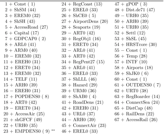
Table 9: Sequence of adaptive LASSO moves for the regional data set without country dum- mies. For further explanations see caption to Table 1.

24

β ˆ

sd

t

Const 0.137260 0.015585 8.807341

GDPCAP0 −0.013651 0.001338 −10.200151 POPDENS0 −0.001199 0.000477 −2.515615 EMPDENS0 0.000994 0.000532 1.866949 TELF −0.001817 0.000382 −4.751923 Capital 0.014913 0.001561 9.554349 AccessAir 0.001922 0.000759 2.532330 AccessRoad −0.004275 0.000897 −4.766852

EREM0 0.053841 0.013324 4.040781

URH0 0.004418 0.003236 1.365442

ARH0 0.026378 0.010716 2.461560

ARM0 −0.066799 0.016054 −4.160842 ARL0 −0.021440 0.006466 −3.315817

ART0 0.015002 0.010627 1.411647

ShSH 0.058186 0.008681 6.702530

ShSM 0.010513 0.005530 1.901018

shGFCF 0.002761 0.001041 2.652060

Table 10: Estimation results for regional data set without country dummies. For further explanations see caption to Table 2.

25

1 + Const ( 1) 25 + URH0 (35) 49 + Dist.de71 (47) 2 + ShSM (44) 26 + ShCE0 ( 5) 50 + gPOP ( 3) 3 + EREM0 (32) 27 + AirportDens (20) 51 + EREL0 (33) 4 + ShSH (43) 28 + Seaports (19) 52 + ShJK0 ( 6) 5 + AccessRoad (27) 29 + Xceec (50) 53 − URH0 (35) 6 + Capital (17) 30 − ART0 (42) 54 + Temp (28) 7 + GDPCAP0 ( 2) 31 − ARL0 (41) 55 + ARH0 (39) 8 + ARM0 (40) 32 + RegObj1 (16) 56 + HRSTcore (30) 9 + ARL0 (41) 33 + ERET0 (34) 57 + INTF (10) 10 − EREM0 (32) 34 + ART0 (42) 58 + ShSL (45) 11 + TELF (11) 35 + RegPent27 (15) 59 − Const ( 1) 12 + ERET0 (34) 36 + ARL0 (41) 60 + Settl (12) 13 + EREM0 (32) 37 + Hazard (29) 61 + URH0 (35) 14 + EREH0 (31) 38 − EREL0 (33) 62 + URT0 (38) 15 + ARH0 (39) 39 + ShLLL (46) 63 + OUTDENS0 ( 7) 16 − EREH0 (31) 40 + URM0 (36) 64 + Airports (18) 17 + POPDENS0 ( 8) 41 + RoadDens (21) 65 + Const ( 1) 18 + ART0 (42) 42 − ARL0 (41) 66 + RegBoarder (14) 19 − ERET0 (34)

43 + ShAB0 ( 4) 67 + DistCap (48) 20 + AccessAir (25) 44 + URL0 (37) 68 + AccessRail (26) 21 + shGFCF (49) 45 + ConnectAir (23) 69 + ConnectSea (24) 22 + EMPDENS0 ( 9) 46 + EREH0 (31) 70 + RailDens (22) 23 + EREL0 (33) 47 + ARL0 (41)

24 + RegCoast (13) 48 − ARH0 (39)

Table 11: Sequence of adaptive LASSO moves for the regional data set with CEEC dummy.

For further explanations see caption to Table 1.

β ˆ

sd

t

Const 0.137147 0.012897 10.633644

GDPCAP0 −0.013149 0.001166 −11.273019 POPDENS0 −0.000275 0.000283 −0.971740 TELF −0.001591 0.000312 −5.106573 Capital 0.014815 0.001457 10.166491 AccessRoad −0.003779 0.000795 −4.750508

EREM0 0.045753 0.012256 3.733273

ARH0 0.021610 0.007691 2.809590

ARM0 −0.058381 0.014855 −3.930148 ARL0 −0.018546 0.005225 −3.549755

ART0 0.012012 0.007729 1.554143

ShSH 0.056410 0.008068 6.992125

ShSM 0.011894 0.005090 2.336598

Table 12: Estimation results for regional data set with CEEC dummy. For further explana- tions see caption to Table 2.

26

Authors: Ulrike Schneider, Martin Wagner

Title: Catching Growth Determinants with the Adaptive LASSO

Reihe Ökonomie / Economics Series 232

Editor: Robert M. Kunst (Econometrics)

Associate Editors: Walter Fisher (Macroeconomics), Klaus Ritzberger (Microeconomics)

ISSN: 1605-7996

© 2008 by the Department of Economics and Finance, Institute for Advanced Studies (IHS),

Stumpergasse 56, A-1060 Vienna • +43 1 59991-0 • Fax +43 1 59991-555 • http://www.ihs.ac.at

ISSN: 1605-7996