Capital and Goods Market Integration and the Inequality of Nations

IHS Economics Series Working Paper 66

June 1999

Capital and Goods Market Integration and the Inequality of Nations

Martin Wagner

Impressum Author(s):

Martin Wagner Title:

Capital and Goods Market Integration and the Inequality of Nations ISSN: Unspecified

1999 Institut für Höhere Studien - Institute for Advanced Studies (IHS) Josefstädter Straße 39, A-1080 Wien

E-Mail: o ce@ihs.ac.atffi Web: ww w .ihs.ac. a t

All IHS Working Papers are available online: http://irihs. ihs. ac.at/view/ihs_series/

This paper is available for download without charge at:

https://irihs.ihs.ac.at/id/eprint/1172/

Institut für Höhere Studien (IHS), Wien Institute for Advanced Studies, Vienna

Reihe Ökonomie / Economics Series No. 66

Capital and Goods Market Integration and the Inequality of Nations

Martin Wagner

Capital and Goods Market Integration and the Inequality of Nations

Martin Wagner

Reihe Ökonomie / Economics Series No. 66

June 1999

Martin Wagner

Institut für Höhere Studien Stumpergasse 56, A -1060 Wien Fax: ++43/1/599 91-163 Phone: ++43/1/599 91-155 E-mail: mwagner@ihs.ac.at

Institut für Höhere Studien (IHS), Wien

Institute for Advanced Studies, Vienna

The Institute for Advanced Studies in Vienna is an independent center of postgraduate training and research in the social sciences. The Economics Series presents research done at the Economics Department of the Institute for Advanced Studies. Department members, guests, visitors, and other researchers are invited to contribute and to submit manuscripts to the editors. All papers are subjected to an internal refereeing process.

Editorial Main Editor:

Robert M. Kunst (Econometrics) Associate Editors:

Walter Fisher (Macroeconomics) Klaus Ritzberger (Microeconomics)

Abstract

A 2-country model with two groups of agents, workers and capitalists is presented in which economic integration results in an initial phase of catch-up, where the less industrialised country experiences the rise in both capital and labour income. Then, after a certain level of integration has been reached, the less industrialised country is completely de-industrialised.

This has detrimental effects on the income of this country's workers, but the capital owners of this country gain from specialisation, as do the workers in the industrialised country. Both the capital and the goods markets are subject to imperfections. The structure of the equilibrium sets during integration is characterised completely.

Keywords

Globalisation, trade, market imperfections, integration

JEL Classifications

F12, F15

Comments

I acknowledge comments by F. X. Hof, L. Kaas, K. Neusser, K. Ritzberger, A. V. Venables, and seminar participants at the University of Technology, Vienna, the University of Economics and Business Administration, Vienna, and at the Institute for Advanced Studies, Vienna. All the remaining errors and shortcomings are of course mine.

Contents

1 Introduction 1

2 Description of the Model 3

3 Equilibrium Structure: Wages, Interest Rates and Income 8

4 Market Integration 13

5 Final Remarks 17

A The perfectly asymmetric case 18

B Some Comparative Statics 18

References 22

1 Introduction

This paper extends the model described in Krugman and Venables (1995) and, in a slightly dierent way, in Fujita, Krugman and Venables (1998). It includes capital as an additional factor of production and it identies capital owners as a distinct group of agents. In addition to transportation costs, the paper introduces imperfect capital mobility as a further wedge between countries.

Krugman and Venables (1995) present a 2-country model that predicts a U-shaped pattern of real incomes during successive phases of economic integration of core and periphery regions. This pattern is meant to rationalise changing positions in the dis- cussion of the eects of (global) economic integration. In the 1960s and 1970s many people argued that integration would harm the developing countries, whereas in re- cent years many people have come to believe that the dicult economic situation in the OECD countries has been aected by market integration that has favoured newly industrialised countries, as for example the countries of South East Asia.

The modelling device that generates this outcome is a model with intermediate goods and transportation costs, which is based on Krugman (1980) and Ethier (1982).

The usage of intermediate goods in the manufacturing sector creates linkages. First, so called forward linkages: a greater variety of intermediate products available reduces the production costs. The costs are lowered the more, the more goods are produced in the same country, because they are not subject to transportation costs. Second, there are backward linkages in which an increase in the share of manufacturing in one country, i.e.

more rms, increases the demand for all the varieties produced in this country through higher demand for intermediate usage by all the other rms in the same country.

To this, we add imperfectly mobile capital owned by another group of agents named capitalists. This simplied set-up perfectly splits investment from consumption deci- sions. The capitalists are only interested in maximising their return on investment and do not take into account the eects of their decisions on the workers' income.

The restrictions to capital mobility in the model shall grosso modo reect all the restric- tions that are prevalent in the real world, like quantitative restrictions to capital import and export,

costs of monitoring foreign investment,

and maybe risk considerations

1

A variant of this model has been used to analyse issues of industrial clustering, see Krugman and Venables (1996).

2

It may be regarded as a nice interpretation to consider the capitalists as a nancial sector that is investing the savings of the consumers and does not take into account the repercussions of their decisions, which mostly arise from the eects of investment on labour income, on the owners of the capital. This interpretation comes rather close to the popular fear that a globalised nancial sector is controlling the real sides of the economies without any control. If it appears more convenient, one can think of two classes of individuals, proletarians and capitalists.

3

Up to some years ago many countries did have tight quantity constraints on the import and export of capital. And if one is thinking over longer horizons of course all the former communist countries have more or less been isolated from the western nancial markets.

4

Like having a lawyer or an investment bank that is taking charge of the foreign investment.

associated with foreign investment.

Parallelling the approach of Krugman and Venables, we will think of a sequence of equi- libria parameterised by declining market restrictions, to assess the eects of continuing integration. The sequences may be best thought of as sequences of steady states, which again shows that the model is intended to analyse long-term developments.

It turns out that the model has a continuum of equilibria. All the equilibrium sets are characterised and analytical expressions for all equilibria are given for all the variables except the price indices (and therefore the real wages). The numerical computation of the price indices is also described.

Following the popular idea that the (uncontrollable) nancial sector is controlling the worldwide evolution of economies, the sequence of equilibria that is analysed is the capitalists' income maximising sequence. This means that given the state of integration the capitalists (of country 1) have the power to choose the equilibrium that gives them the largest income.

This leads to the following pattern of industrial agglomeration: In a situation with large restrictions one country is specialised in manufacturing whereas the other country is active on both sectors. During the rst stage of integration, the manufacturing sector is shrinking in the industrialisedcountry and growing in the other one. This corresponds to the situation that is seen as a threat to high living standards in industrialised countries today. This phase is characterised by a rising income of workers and capitalists in the country that experiences industrialisation.Later, after the restriction to capital mobility has dropped below a critical value, all the worldwide manufacturing is concentrated in one country. This has severe adverse eects on real income of the workers in the de- industrialised country, while it has positive eects on the real income of the workers in the country that has captured the whole manufacturing sector. During the course of integration, the income of the capital owners of the two countries is equalised. In this model integration thus favours the owners of the mobile factor capital in contrast to the immobile factor labour. Thus workers living in the country which has managed to attract the manufacturing sector therefore happen to prot from the process of economic integration.

Section 2 describes the model. In Section 3 the equilibrium structure is described, in

5

Our model has no risk. One can, however, still regard risk as a factor that reduces the eective, or average, rate of return on investment.

6

Due to the fact that there is a continuum of equilibria an equilibrium has to be chosen at each point of the integration process. In our model the most intrinsically consistent choice is to choose the equilibrium that maximises the return on investment. The results do not change qualitatively if the worldwide income of capitalists is taken as the criterion for selecting equilibria. Besides the above,

"natural" candidates would be equilibria with a specied allocation of revenue between capitalists and workers, or equilibria maximising a social welfare function at each point of the sequence. It may also be an interesting task to compare these equilibrium sequences.

This equilibrium selection can be interpreted as the result of a limiting bargaining situation in which

the capitalists have all the bargaining power.

Section 4 the sequence of equilibria during ongoing integration is discussed and Section 5 presents some nal remarks. There are two appendices. In Appendix A a special case of an equilibrium that can be treated analytically is shortly discussed and Appendix B reports all the comparative statics results.

2 Description of the Model

In my presentation I closely follow the lines of Fujita, Krugman and Venables (1998).

The world is assumed to consist of two economies which will be labelled 1 and 2 through- out the paper. Subscripts are used to refer to the countries. The two countries are iden- tical with respect to their endowments of labour, capital and the available technology.

In each country there are two types of agents: consumers (workers) and capitalists. The countries are also identical with respect to the preferences of consumers and capitalists.

The following description omits country indices if the described relationship holds for both countries. Where necessary, countries will be distinguished.

The workers in the economies all share the same preferences

V = M A

(1)

where A is the consumption of the agricultural good and M is a quantity index of manufactured goods consumption. Both countries are endowed with a total of L = 1 units of labour. Labour is perfectly mobile between the two sectors and completely immobile across the two countries. The agricultural good is taken to be the numeraire, i.e. its price is set to one. is the constant expenditure share of manufactures. M is dened over a continuum of varieties of manufactured goods

M = (

^N

0

m ( i ) di )

⁼ ; 0 < < 1 (2) where m ( i ) denotes the consumption of the variety i and N is the range of varieties produced. is a parameter reecting the preference for variety. The smaller the larger the preference for variety. This formulation has been popularised by Dixit and Stiglitz (1977).

The representative consumer's problem, given income Y and all the prices p ( i ), can be solved in two steps, because the consumer preferences are separable between agriculture and manufacturing. First one has to minimise the expenditures necessary to obtain M , for any given value of M . This results in demands m ( j ) = ^p

^j

[ RN

0

p

i

di

M for all the dierent varieties m ( j ). Multiplying m ( j ) with its price p ( j ) and integrating over all the varieties yields

Z

N

0

p ( j ) m ( j ) dj = [

^N

0

p ( i )

di ]

M (3)

The term multiplying M on the right hand side of equation (3) can be interpreted as a

price index. This interpretation implies that the expenditure on manufacturing is equal

to the price index of the composite good times the quantity index of consumption of manufactured goods.

Dening =

, gives P = [

^N p ( i )

di ]

= [

^N p ( i )

di ]

. >From the Cobb- Douglas preferences, we immediately know the allocation of income between M and A : M = Y=P and A = (1

) Y . Substituting this expression shows that the consumer demand for each of the varieties of manufactures is given by m ( j ) = Y ^p _P

^j

;

j

[0 ;N ]. The consumers' sole source of income is labour, so Y = w , where w is the nominal, i.e. measured in units of the agricultural good, wage. Real wage ! , i.e. nominal wage divided by the consumer price index, is given by

! = wP

(4)

The agricultural good is tradable without transportation costs. This implies that there is one worldwide market for the agricultural good. The manufactured goods are subject to transportation costs. For simplicity these costs are modelled as iceberg transport costs:

only a fraction _T

, T

1, of a unit shipped, arrives in the other country. With a simple specication like this, we avoid the necessity to model an additional transportation industry. So, if a specic variety k is produced in country 1, its prices in 1 and 2 are given by p

( k ) = p

( k ) T .

In equilibrium all varieties produced in one country must sell at the same price, because they enter utility symmetrically and are produced with the same technology. Thus, the manufacturing price indices can be expressed as

P

= ( n

p

+ n

( p

T )

)

(5) P

= ( n

( p

T )

+ n

p

)

(6) where n i denotes the "number" of varieties produced in country i and P i stands for the price indices in the two countries.

The capitalists in the two economies are endowed with W

= W

=

units of capital. In this paper we will use K i for the amount of capital employed in country i .

The capitalists' sole objective is maximising the return on capital.

Capital is imper- fectly mobile. In this paper we model the restrictions on capital mobility in a fashion similar to the transportation costs prevalent on the manufactured goods markets. In each country there is only one capital market, i.e. there are no separate markets for capital owned by either domestic or foreign investors. This implies that there is only one interest rate per country. Now for each unit of capital invested abroad an investor

7

The parameters

and

will appear later in the production function for manufactures. This choice of endowment with capital turns out to be very convenient when solving for equilibrium.

8

This need not be equal to

, the amount of capital owned by the capitalists resident in the country

i

. Let

denote the amount of capital owned by capitalists resident in

that is invested in the country

j

. Then of course

+

= (

+

) + (

+

) =

+

has to hold (in equilibrium).

9

With this simple specication the capitalists are only interested in obtaining as much of the nu-

meraire, i.e. of the agricultural good, as possible. Therefore there are no demand eects on the manu-

factured goods market from this side.

does not earn r units of the agricultural good, but only r=U , with U being

1, units.

Solving the problem of the representative capitalist (resident in country 1) trivially leads to the following capital supply function:

W

^S =

8

>

>

<

>

>

:

W

if r

> r

=U

2

[0 ;W

] if r

= r

=U 0 if r

< r

=U

The incomes of capitalists resident in country 1 and 2 are given by C

= r

W

+ r

U W

⁽⁷⁾

C

= r

U W

⁺ r

W

(8)

Next we turn to the description of the behaviour of the producers in the economy. Agri- culture uses only labour as an input and is assumed to be a perfectly competitive CRS sector. For simplicity, the agricultural good is produced with a linear technology, where normalisation is such that one unit of labour is producing one unit of the agricultural good. The economy-wide production of agriculture is then given by A = (1

), where denotes the share of labour of the economy devoted to manufacturing.

Manufacturing is a monopolistically competitive IRS sector that uses labour, capital and intermediate goods as inputs to produce the varieties of manufactures. Technology is Cobb-Douglas and assumed to be identical for all the varieties and both countries.

The scale eects thus occur at the level of production of the dierent varieties. For this reason, and because we assume free entry and exit and an unlimited potential of vari- eties, two competitive rms won't choose to produce the same variety. The production function of an operating rm is given by

F + cq = Dl

k [

^N

0

g ( i ) di ] ⁼ (9) where q is the quantity produced, l the amount of labour used, k the amount of capital used; the integral term represents the quantity index of the manufactured goods used as intermediates. g ( i ) denotes the quantity used of variety i . With this specication of intermediate demand of the rm sector, we nd that the intermediate composite good used as an input in production has the same composition as the aggregate of manufactured varieties demanded by the consumers (in the same country). This set-up is convenient when deriving total demand for manufactures. F stands for the xed costs that an operating rm incurs, c is the marginal input requirement.

Firms are prot maximising, price takers on their input markets and price setters on their output market. Furthermore, when taking their decision, rms consider the price index P xed. The prot function of a rm is given by

( i ) = p ( i ) q ( i )

w

r P ( F + cq ( i )) (10)

10

The constant

is set to (

)

(

)

(

)

.

where p ( i ) denotes the price of the produced variety, q ( i ) the quantity produced and w and r are the wage and interest rates.

Taking into account the pricing behaviour of the monopolistic rm and noting that is the elasticity of demand perceived (keeping P xed) , p (1

) = w

r P c has to hold. Choosing units so that c = (1

) we obtain

p = w

r P (11)

Inserting the price in the prot function yields = w

r P [ ^q

F ]. Free entry drives prots down to zero in equilibrium, so that the equilibrium quantity produced by all the rms is q

= F .

The technology described above implies that every rm uses all the varieties of ma- nufactured products as intermediates. So the producers, as well as the consumers gain from having a larger worldwide variety of manufactured goods. This is a forward link- age. In addition, as already mentioned in the introduction, the larger the share of varieties produced in one country, the larger the reduction in the price index that the rms (and consumers) experience in this country, because less varieties are subject to transportation costs.

Now we collect all the equations and identities describing equilibrium. The income of the workers Y is the sum of workers' earnings in agriculture and in manufacturing

Y = (1

) + w (12)

Y can exceed one only if all labour is devoted to manufacturing and manufacturing pays a wage higher than one. Total expenditure E on manufactures in the two countries is composed of consumer demand - fraction of consumer income - and the rms' intermediate demand - fraction of total costs or, equivalent in equilibrium, of total revenue - and is given by

E i = Y i + n i p i q

The above equation can be modied by using the following equilibrium conditions on factor payments that directly follow from the assumption of the Cobb-Douglas tech- nology.

(1

) n i p i q ^eq = w i i

n i p i q ^eq = r i K i

n i p i q ^eq = P i M i

where K i is the capital employed in country i and M i is the economy wide intermediate

demand in i . Now choose units so that q

=

, i.e. set F to

. Then

P i M i =

w i i and n i = ^w _p

. The (gross) interest earned on capital in country i

is then r i K i =

w i i . Because of imperfect capital mobility, this only equals the

amount that the owners of the capital get paid, if there is no cross border investment or

the restrictions are degenerated, i.e. U = 1. Using the above expressions, the expenditure equation can be expressed as

E i = Y i +

1

w ⁱ i (13)

The above normalisations have been made because the focus is on the allocation of labour between the sectors and on the allocation of capital between the countries, not on the number of rms or the prices.

Inserting the above relations, we can express the price index for country 1 (analogous for country 2) as

P

= ( n

p

+ n

( p

T )

)

= ( w

p

+ w

p

T

)

= ( w

( w

r

P

)

+ w

( w

r

P

)

T

) (14) Use r i K i =

w i i , dene ~ K i = K i

to further modify the price index equa- tions to

P

= ( w

K ^~

P

+ w

K ^~

P

T

) (15) P

= ( w

K ^~

P

T

+ w

K ^~

P

) (16) Noting that ~ K

+ ~ K

=

( K

+ K

) =

( W

+ W

) = 1, we see that the quantities ~ K i are the shares of worldwide capital allocated to country i . The demand for a single variety v produced in country one is given by

q ( v ) ^D = E

p

P

+ E

( p

T )

P

T (17) The rst term is the demand for consumption and intermediate usage from country 1, the second term is the demand from the other country. Now we use the fact that rms sell q =

units in equilibrium and the price equation (11) to obtain

( w

r

P

) = (1

)( E

P

+ E

P

T

) (18) ( w

r

P

) = (1

)( E

P

T

+ E

P

) (19) We will refer to the above equations as the wage-interest equations, since they give com- binations of wages and interest rates consistent with zero prots.

For our purposes, it is convenient to rewrite these equations as follows

( w

K ^~

P

) = (1

)( E

P

+ E

P

T

) (20) ( w

K ^~

P

) = (1

)( E

P

T

+ E

P

) (21)

11

In this respect we follow the lines of Fujita, Krugman and Venables (1998). We do not refer to the approach in Krugman and Venables (1995).

12

Fujita, Krugman and Venables derive similar equations without an interest rate term and label

them wage equations .

For completeness' sake, it remains to characterise equilibrium on the agricultural (nu- meraire) market. The worldwide supply of agricultural goods is given by (1

)+(1

). Demand is the sum of two components: Consumption demand, which is given by (1

)( Y

+ Y

), and the (gross) interest payments r

K

+ r

K

. Equating supply and demand gives

(1

) + (1

) = (1

)( Y

+ Y

) + ( r

K

+ r

K

) (22) Finally, in equilibrium capital demand has to equal capital supply in both countries.

3 Equilibrium Structure: Wages, Interest Rates and In- come

When discussing asymmetric equilibria we will focus on the case where country 1 is the more industrialised country.

Dierences in equilibria may depend on whether both countries have both sectors active and on whether there are cross border capital ows.

Of course, in a situation in which all the manufacturing is concentrated in one country, all the capital must have been invested in this country.

Both workers and capitalists gain from a clustering of manufacturing in one country.

The reduction of the price index that is implied by this agglomeration increases the real income of workers ! and the protability of rms via reduced expenditures on intermediates and an increased demand for intermediate usage from other rms located in the same country. If the agglomeration eects are strong, this potentially allows rms in the country with the larger manufacturing share to pay higher interest rates than the rms in the other country, which in turn attracts foreign capital. Of course, it is advantageous for capitalists to be resident in the country that is relatively more specialised in manufacturing and has a higher interest rate. Because only in-owing capital is subject to restrictions on the capital market, the capitalists based in the industrialised country have higher (net) returns than foreign investors.

For all the values of T and U the symmetric situation, in which the two countries are identical with respect to the values of all variables, is an equilibrium. The values of all the variables can be easily determined for this equilibrium. First note that w

= w

= 1 and that therefore Y

= Y

= 1 have to hold because agriculture is active in both countries. Next, use (22) to determine the symmetric =

. Thus we derive

13

Using Walras' law we could skip one market in the description of equilibrium.

14

It is a fairly general feature of the so called New Trade Theory models that there is a substantial amount of indeterminacy due to the usually completely symmetric set-up of the (2-country) models.

The models therefore have the ability to generate asymmetries but they do not endogenously explain

the reason why one symmetric country attains the favourable position rather than the other. According

to our view this is a nice feature of these models because it leaves room for other aspects like culture

or history that cannot be modelled directly to serve as explanatory factors of asymmetric evolution.

E

= E

=

. Now insert the known quantities in (15) ; (16) or (18) ; (19) and use K ~

= ~ K

= 1 = 2 to obtain

P

= P

_{= (12)}

(1 + T

) (23) The interest rate is given by r = 2 =

. The capitalists' income C is equal to

1;

, real wages are given by ! = P

.

We can also prove the existence of a specialised equilibrium. The meaning of special- ized depends on the level of manufacturing necessary to satisfy worldwide demand with manufacturing being either solely concentrated in one country or, if there has to be a larger manufacturing sector, in both countries with one country having only manufac- turing.

As indicated, we will take country 1 to be specialised. To be able to proceed analytically, we will restrict ourselves (at the moment) to an analysis of the case in which all manufacturing goods can be produced by country 1.

Thus, we can still use w

= w

= 1 when solving for equilibrium.

To solve for the values of the variables in a specialised situation, we proceed as follows. From w

= w

= 1 we immediately derive Y

= Y

= 1. We also know by assumption that

= 0 has to hold. Use (22) to determine

=

. For this being smaller (or equal) than one, <

has to hold, i.e. we have to impose an upper bound on the share of manufactures in consumption to guarantee that worldwide demand for manufacturing can be satised by one country.

Next substitute the expression for

in (13) to obtain E

=

and E

= . Now solve for the price indices by inserting in (15) and (16) to get P

=

and P

= P

T . The equation P

= P

T is derived from the fact that in the situation described all the varieties of manufactures have to be shipped from 1 to 2. Real wages are given by !

= P

and !

= !

T

. The capitalists' income is given by C

= r

W

=

and C

= C

=U = _U

.

In this situation workers and capitalists resident in country 1 are better o because they have higher real wages and a higher rate of return.

Now it remains to clarify when this situation is an equilibrium. It can only be an equilibrium when it is not protable to invest in country 2 and start manufacturing production there. This protability question can be decided by looking at the wage-

15

The case where all manufacturing is concentrated in one country can be divided in two sub-cases,

1<

1 and

= 1. The second case will be referred to as the perfectly asymmetric case, where there is only manufacturing in country 1 and only agriculture in country 2.

16

The case with a large manufacturing sector is discussed later on.

17

In the perfectly asymmetric case we still can nd the value of

1 and can also proceed analytically.

18

Strictly speaking one has to choose the parameters

,

and

in a way that this inequality is fullled but the interpretation given in the text is very natural. In the context of the paper of Krugman and Venables, where

would be 0, this condition would be reduced to

.

19

The results for the perfectly asymmetric case are given in Appendix A.

interest equation of country 2 in the context of the specialised situation ( w

r

P

) = (1

)( E

P

T

+ E

P

)

= (1

)(

P

T

+ P

T

) (24) To attract labour, a manufacturing rm planning to start production in 2 has to pay a wage of w

= 1. Using this, P

=

and r

=

(24) further simplies to

r

= r

(1 +

2 T

+ 1

2 T

)

T

(25)

Here r

stands for the maximum interest rate a rm planning to start production in 2 would be able to pay its capital owners while achieving zero prots. This implies that the specialised situation is an equilibrium if

U

> (1 +

2 T

+ 1

2 T

) T

(26)

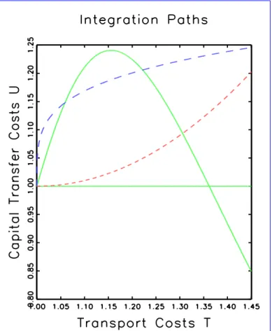
(26) describes the feasible region of T and U , given ;; and , that allow for a specialised equilibrium with w

= 1. See Figure 1 for an illustration.

Within the specialised region (the workers') real income, the capitalists' income and the price level in country 2 vary according to the values of T and U . The equilibrium quantities in country 1 do not vary throughout the whole region, because in the situation described the integration parameters T and U inuence the situation in this country neither on the goods nor on the capital market.

We next describe equilibria which involve manufacturing in both countries and capital ows between the countries.

Two cases have to be distinguished: The case where both sectors, manufacturing and agriculture, are active in both countries, and the case where only manufacturing is active in one country and agriculture and manufacturing are active in the other one. Again we will take country 1 to be the more industrialised country. The existence of equilibria of these types depends on the values of certain parameters. To have capital ows from 2 to 1, the interest rates have to be related by r

= r

U .

Let us rst look at the case where country 1 is specialised in manufacturing and country 2 has agriculture and manufacturing.

We solve for this equilibrium by using the following indirect approach. Regarding the case under investigation, we know that w

either has to equal 1 or has to be larger than one. Thus, we set w

= w with w

1. Using (22), we get

=

(1+ w )

w . For 0

1 w

w max =

has to hold. On the other hand for w max

1, we have to impose

which is the

20

At the end of this section we will also look at equilibria that have an uneven allocation of manu- facturing but no capital ows.

21

So this is the specialised case for a large manufacturing sector. If

, this kind of

equilibrium is possible for all values of

and

, not only for a bounded set like the one described by

equation (26).

Figure 1: The feasible region of T and U allowing for a small specialised equilibrium is bounded by the two solid lines. Parameter values: = 0 : 25, = 0 : 35, = 0 : 5, = 5.

The parabolic dotted lines are two integration paths, i.e. paths of T and U converging to (1 ; 1). The convex curve is given by T = U

2 U + 2, the concave curve is given by T = 0 : 3 U

+ 1.

already familiar restriction for a suciently large manufacturing sector. Use r i K ~ i = w i i

to get ~ K

= _w

^U

_U

. From r

= r

U we know that ~ K

has to be smaller than

or equal to

. This implies that U

U max ( w ) =

^w

_w

_w

. For U max ( w )

1 the condition w

has to be imposed. Combining all the formulas used above, we have equilibria with only manufacturing in 1 and with agriculture and manufacturing in 2 for

, w

[1 ;

] and U

[1 ;U max ( w

)].

Straightforward substitution then yields ~ K

= _w

^w

+

U

, r

= w

+ U

and r

= ^w

_U ^U

. The price indices in the two countries can be found by solving the price index equations which can be transformed to

P

= r

( U

w

P

+

P

T

) (27)

P

= r

( U

w

P

T

+

P

) (28)

using n i p i = w i i and (11).

There is a continuum of equilibria given the parameter values. We have parameterised this equilibrium set by choosing w

. This is equivalent to a specic allocation of the revenue of the manufacturing sector to workers and capital owners because r

is also depending on w

. Therefore the continuum of equilibria arises from dierent possibilities of distributing the manufacturing revenue.

Now equilibria in which both sectors are active in both countries and which involve capital ows between the countries can be found by performing similar manipulations.

Here

is set to an undetermined

. The results are in brief:

<

1

and U

U max (

) =

. We also get r

=

+ U

and ~ K

=

U

. The price indices can now be found by solving

P

= r

( U

P

+

P

T

) (29) P

= r

( U

P

T

+

P

) (30) for P

and P

.

It nally remains to characterise equilibria without capital ows but an uneven allo- cation of manufacturing to the two countries. First we note that there are no capital ows for r

=U < r

< r

U . We can therefore write r

= r

S for S

( _U

;U ). This implies

=

_S

and

=

_S

^S

.

Also 0 < i

1 has to hold which is guaranteed by

1 < S <

, i.e. we have bounds on the value of S that support equilibria of this type. The other variables are found by inserting i

and r i in the corresponding equations, the price indices are now found by solving P

= 2

(

P

+

P

T

) (31) P

= 2

(

P

T

+

P

) (32) In all the above cases the modied price index equations can be dierentiated with respect to P

, P

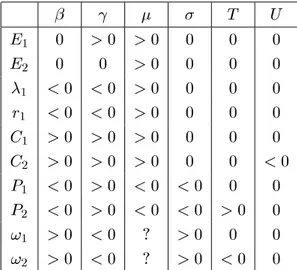
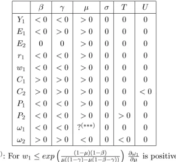
, T and U in order to get the comparative statics of the price indices (and therefore real income) with respect to all the parameters evaluated at these equilib- ria.

Comparative statics for all the other variables is straightforward since analytical expressions are available for them.

22

Technically the non-uniqueness of equilibrium stems from non{(strict){convexities like linear tech- nology in agriculture, the demand of capitalists and xed costs in manufacturing. As we have seen before, the linear specication of the capitalists leads to a capital supply function that is indeterminate for equal net interest rates between the two countries.

23

We assume again

. For

the same reasoning applies with

1

2^(1;;)

1;

. This type of equilibrium is of course possible for manufacturing sectors of any size.

24

For country 1 being the country with the higher interest rate, we have to restrict

to be in (

1).

25

As usual we assume

. The values of S that are feasible are

(

)

(

1

). The case

can be handled in a completely similar way.

26

Because the price indices are found numerically one has to insert the numerical values of

and the analytically given values of the other variables into two- dimensional systems of linear equations.

See Appendix B .

4 Market Integration

In this section we report the consequences of economic integration on the two countries by drawing on the results from Section 3.

We assume that the capitalists do have the power to choose the equilibrium that max- imises the return on investment, i.e. there are no legal or institutional restrictions on the actions of the capitalists.

Another interpretation is that this equlibrium selection is the result of a bargaining process where all the bargaining power is in the hands of the capitalists.

>From the preferences of the capitalists, it follows that only the imperfections on the capital market, given by U , exert inuence on their choices. The paths have a structure as described in the following table where we see the dependence of the chosen equilibrium on U .

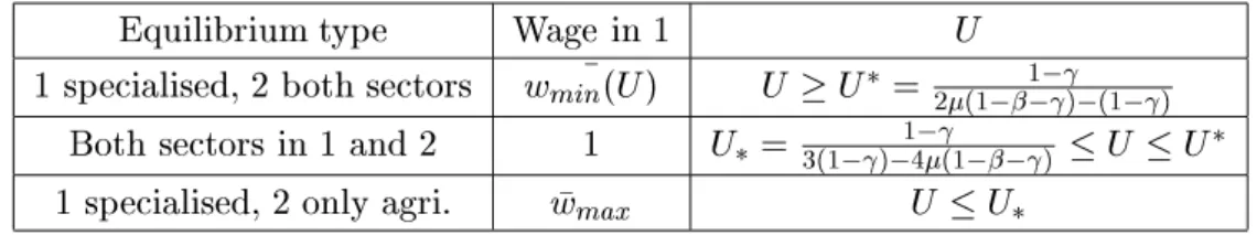
Table 1: The capitalists' income maximising equilibria during economic integration.

In this table the term specialised means that the country has devoted all labour to manufacturing.

Equilibrium type Wage in 1 U

1 specialised, 2 both sectors w min ( U ) U

U

=

Both sectors in 1 and 2 1 U

=

U

U

1 specialised, 2 only agri. w max U

U

It is interesting to note that for U

U

, the optimal (nominal) wage level set by the capitalists is the maximum possible wage which leads to the limiting case

( w

) = 0 in this situation.

So all the capital owned by capitalists resident in country 2 is invested in country 1. This means that for U

U

, the interest rate that can be generated by concentrating all the manufacturing is large enough to make foreign investment protable. The high wages are accompanied by high prices which are the basis for gen- erating higher interest rates than in a situation where manufacturing would be allocated to both countries.

This set-up implies that according to the investment decisions taken by capital owners who decide about industrial agglomerations workers are directly inuenced by integra- tion on the goods markets and indirectly by integration on the capital market. In the

27

One could e.g. think of unions that may inuence wage negotiations or the like.

28

See the discussion after Figure 3 for what is happening when bargaining power is attached to both groups.

29

wmin

(

) =

. The above table assumes

, for

larger than this value country 1 will be specialised throughout the whole sequence of integration, and country 2 will have both sectors for

and only agriculture for

smaller than this value.

30

In this section the sequence of equilibria is computed along the concave path shown in Figure 1 .

Of course any path (

)

(1

1) serves the same purpose, but this one is already drawn in Figure 1 .