Many-Body System

Classical and Quantum Signatures of Quantum Phase Transitions in a (Pseudo) Relativistic

Many-Body System

Maximilian Nitsch *, Benjamin Geiger *, Klaus Richter * and Juan-Diego Urbina * Institut für Theroretische Physik, Universität Regensburg, 93040 Regensburg, Germany

* Correspondence: maximilian.nitsch@physik.uni-regensburg.de (M.N.);

benjamin.geiger@physik.uni-regensburg.de (B.G.); klaus.richter@physik.uni-regensburg.de (K.R.);

juan-diego.urbina@physik.uni-regensburg.de (J.-D.U.)

Received: 6 March 2020; Accepted: 2 April 2020; Published: 4 April 2020

Abstract:We identify a (pseudo) relativistic spin-dependent analogue of the celebrated quantum phase transition driven by the formation of a bright soliton in attractive one-dimensional bosonic gases. In this new scenario, due to the simultaneous existence of the linear dispersion and the bosonic nature of the system, special care must be taken with the choice of energy region where the transition takes place. Still, due to a crucial adiabatic separation of scales, and identified through extensive numerical diagonalization, a suitable effective model describing the transition is found.

The corresponding mean-field analysis based on this effective model provides accurate predictions for the location of the quantum phase transition when compared against extensive numerical simulations.

Furthermore, we numerically investigate the dynamical exponents characterizing the approach from its finite-size precursors to the sharp quantum phase transition in the thermodynamic limit.

Keywords: phase transitions; semiclassical approximation; Dirac bosons; mean field analysis;

adiabatic separation

1. Introduction

The methods and ideas of quantum chaos [1,2] provided deep insights into the way classical information conspires with ¯hin a subtle manner. To a large extent, this can be understood within a semiclassical theory, explaining genuine quantum behaviour, such as entanglement and coherence.

In this field, Shmuel Fishman made paramount contributions ranging from the celebrated explanation of dynamical localization as a type of Anderson transition in kicked systems [3] to the resummation of periodic orbit expansions to construct semiclassical approximations for individual eigenstates in chaotic systems [4]. The present contribution aims to express our admiration for his scientific work.

During the last decade, the field of quantum chaos experienced an influx of new ideas coming from its application to the realm of interacting many-body systems. The newly emerging field of many-body quantum chaos is based on exciting developments in our understanding of fundamental problems, such as the equilibration of closed systems [5–9] and the scrambling of quantum information due to classical chaos [10–13].

It is, therefore, not a surprise that semiclassical methods, both at the heuristic level of quantum-classical correspondence [14–16] and the level of asymptotic analysis of path integrals describing coherent quantum effects [17–21], were lifted from their original particle-like form into the realm of quantum fields. Among the plethora of phenomena characteristic of the rich physics of interacting many-body systems, critical phenomena have always had a special place. In this new disguise, many-body semiclassical methods are a suitable tool to understand even the most delicate quantum effects related to the emergence of criticality.

Condens. Matter2020,5, 26; doi:10.3390/condmat5020026 www.mdpi.com/journal/condensedmatter

A natural arena for testing this idea is the attractive Lieb-Liniger model [22] describing one-dimensional bosons attractively interacting through short-range forces and, in particular, its low-energy effective description that was experimentally realized [23,24]. The reason for this is that this system displays a quantum phase transition [25–28] and admits a proper semiclassical derivation of a well-defined and controlled classical limit in the form of mean-field equations, thus allowing for direct application of semiclassical techniques [21]. The semiclassical study of this system in [21] revealed the key role played by locally unstable mean-field dynamics in the corresponding dynamical and spectral quantum mechanical features.

The extension of many-body semiclassics beyond the realm of bosonic systems is still in its infancy, but a step in this direction is to first consider how the well-established picture of [21] gets modified by two new ingredients: a relativistic dispersion and the presence of spin-like degrees of freedom.

Since the very possibility of having locally unstable dynamics (as opposed to global chaos) of the attractive Lieb-Liniger model is due to the integrability of the effective Hamiltonian describing its low energy regime, a natural question concerns possible non-integrable behaviour of such models and its consequences for the existence and characteristics of the quantum phase transition. In this paper, we answer some of these questions.

The paper is organized as follows. After we introduce the model and describe its general physical properties in Section2, we present the motivation for the transformation into a special Fock basis in Section3and how this optimal transformation adiabatically fragments the Hamiltonian in Section4.

After that, in Section5, the conversion of the channel containing the ground state into its classical form is examined. The most important results presented in the Section6are the exact calculation of the critical interaction strength and the analysis of discontinuities in the functional dependence of the energy on the interaction. Finally, the asymptotic convergence of the first excited energy level towards the ground state level leading to a degenerate ground state in the mean field is quantified in Section7.

2. The Hamiltonian and Its Symmetries

The Hamiltonian of the (modified) Lieb-Liniger model with linear dispersion and contact potential is defined as

Hˆ

=

−i¯h

∑

N β=1

∂ˆ_β⊗σˆ_z^(β)− ^Rα 4

∑

N β,γ=1

δ

(

xˆ_β−xˆγ

)(

σˆ_x^(β)

+

σˆ_x^(γ)

)

, (1) describing bosons on a ring with radiusRwith a contact interaction that can be interpreted as a mass term: The moment two bosons are at the same point they obtain a mass through the contact potential, whereas they are massless otherwise. In the following we assume attractive interactions, e.g.,α>0, and we will choose natural variables ¯h

=

1,L

=

2πR

=

2πsuch that the unit of energy is

[

E

] =

_R^¯h [28].

As appealing as it is, it is important to note that the system above appears ill-defined, as its Hamiltonian (1) is not bounded from below. Unlike in fermionic systems, in this bosonic system this issue cannot be resolved by the introduction of a Fermi sea. One way out of the problem is to interpret (1) as emerging from a local approximation of a one-dimensional condensed matter or cold atom system with two crossing bands that is perturbed by an interband interaction. This naturally introduces a regularization of the noninteracting model with a single-particle momentum cutoff defining the region where the linearization is justified. In this approach, the linear dispersion is a property of excited states and has an effect on dynamical properties of states with a certain momentum.

An example of such (local) Dirac bosons in two dimensions was found in the collective plasmon dispersion relation in honeycomb-lattices of metallic nanoparticles [29]. In such local approximation, one has to make sure that any prediction of the model has to be independent of the cutoff, which might be realized in a quench scenario, starting with a narrow momentum distribution.

However, we take a different perspective here that takes a truncated model as it is, i.e., we truncate to the three lowest single-particle momentum modes (for each quasi-spin, see below) and then assume that the ground state of this model represents a physical ground state. One possible realization of such a system is obtained by mapping the truncated model to a spin-one bose gas on two quantum

dots (or two sites with suppressed hopping), where the physical spin takes the role of the momentum k

=

−1, 0, 1 and the pseudo-spin 1/2 labels the two sites that have opposite external magnetic fields applied to them, introducing linear Zeeman splitting and thus the “three-mode linear dispersion”.

The interaction processes are then taking, e.g., two particles of opposite spin on the same site and distribute them into the spin-zero modes of the two sites. There are different processes, of course, but the overall interaction effect is a spin-mediated hopping of a single particle with the total spin (of the participating particles) being preserved. The noninteracting case would decouple the two sites.

To implement the truncation within a Fock space approach, we choose the eigenbasis of the non-interacting (α

=

0) Hamiltonian as the single-particle basis

|k,σi

=

|ki ⊗ |σi, (2) where as orthonormal eigenbasis for the momentum operator we use plane waves

hx|ki

=

√¹

2πe^ikx, withk∈Z (3)

as the most obvious choice. For the quasi-spin an orthonormal eigenbasis is used consisting only of

“up” and “down”

σ∈ {+1,−1}, |σi ∈ ( 1

0

! , 0

1

!)

(4) generated by the third Pauli-matrix

ˆ

σ_z|σi

=

σ|σi. (5)

From these definitions the Fock space is characterized through the occupation numbersn_k,σof the several states|k,σiwith creation and annihilation operators satisfying canonical commutation relations

[

aˆk,σ, ˆa^†_l,τ

] =

δ_k,lδσ,τ,

[

aˆk,σ, ˆal,τ

] =

0,

[

aˆ^†_k,σ, ˆa^†_l,τ

] =

0, (6) where each pair of creation/annihilation operators defines an occupation number operator

lnˆ_k,σ

=

aˆ^†_k,σaˆ_k,σ (7) for the corresponding mode. With the help of these bosonic operators this leads, after truncation of the momenta fromZ^to{−1, 0, 1}, to the more convenient form

Hˆ

= ∑

k∈{−1,0,1} σ∈{−,+}

σk·aˆ^†_k,σaˆ_k,σ−^α

2

∑

k,l,m,n∈{−1,0,1} σ,τ∈{−,+}

ˆ

a^†_k,σaˆ^†_l,τaˆm,−σaˆn,τ·δ_k+l,m+n, (8)

with the relevant Fock states labeled by six occupation numbers,

|n1,+,n0,+,n−1,+,n1,−,n0,−,n−1,−i. (9) This Hamiltonian has a set of symmetries that will be the key for the adiabatic separation later on.

We have the total number of particles

Nˆ

= ∑

k∈{−1,0,1} σ∈{−,+}

ˆ

n_k,σ, (10)

and the total angular momentum

Lˆ

= ∑

k∈{−1,0,1} σ∈{−,+}

k·nˆ_k,σ. (11)

Using (8), it is easy to show that

[

H, ˆ^ˆ N

] = [

H, ˆ^ˆ L

] =

0, (12) and the Hilbert space can be divided into sectors with the respective quantum numbers

(

N,L

)

. To simplify the task we will focus on the special case of fixedNandL

=

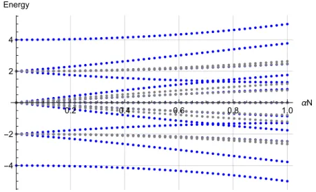
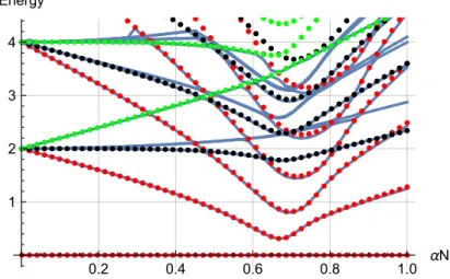
0. Except for the derivation of the effective Hamiltonian which is done for generalL. In this way, the effective number of degrees of freedom is reduced from six to four.

Besides these two symmetries, the energy spectrum splits up symmetrically in the positive and negative direction, as can be seen in Figure1. For an even particle numberNthis observation can be explained using the operator

ξˆ

=

⊗^N_α=1σˆ_x^(α)

(−

1

)

^S2ˆ (13) where ˆSis the total (pseudo) spin

Sˆ

=

∑

N α=1

ˆ

σ_z^(α) (14)

that satisfies

(−

1

)

^S2ˆ ·

(−

1

)

^−S2ˆ

=

1, (15) and therefore it is easy to show that

hψ|ξ^ˆ†Hˆξˆ|ψi

=

− hψ|H^ˆ |ψi. (16) As ˆξis a bijection on the set of eigenstates|ψiof ˆHwith energyE

=

hψ|H^ˆ|ψi, there always exists a state|φi

=

ξ^ˆ|ψithat is also an eigenstate of ˆH. The energy value corresponding to this state is then given by

E_φ

=

hφ|H^ˆ|φi

=

−E. (17) Finally, a parity operator ˆPcan be defined which simultaneously flips all spins and momenta, given by a complex conjugation to invert the momenta in the eigenbasis of plane waves followed by a spin flip,

Pˆ

=

⊗_α=1^N σˆ_x^(α)

(·)

^∗, (18) satisfying ˆP²

=

1. Also, since

[

P, ˆ^ˆ H

] =

0, ˆPrepresents a discrete symmetry that splits the Hilbert space into two separate subspaces leading to a separation of the energy spectrum into two independent subspectra (In general, one does have

[

P, ˆ^ˆ L

]

6=0; however, forL

=

0 the two operators commute.)

H

=

^{H+ 0} 0 H−

!

, (19)

see Figure1.

0.2 0.4 0.6 0.8 1.0 αN

-4 -2 2 4 Energy

Figure 1.Energy spectrum forN=4,L =0 splitted into positive (blue) and negative (gray) parity.

Scaled units[E] = _R^¯h used.

As a final remark, we note that the existence of further symmetries is ruled out by a numerical diagonalization and the analysis of avoided crossings, as indicated for N

=

_20,L

=

_0, P

=

_{1 in} Figure2. The absence of real crossing suggests that there are no additional symmetries to be found which could be used to further reduce the dimensions of the Hamiltonian (8) [30].

0.2 0.4 0.6 0.8 1.0

αN 1

2 3 4 5 Energy

point 1 point 2

0.3642 0.3644 0.3646 0.3648 0.3650 αN 2.697

2.698 2.699 2.700

Energy

0.825 0.830 0.835 0.840 αN 3.86

3.88 3.90 3.92

Energy

Figure 2.Excitation spectrum atN=120,L=0 (left) and zooms into two exemplarily points which display avoided crossings (right). Scaled units[E] = _R^¯h _used.

3. Adiabatic Separation of the Hamiltonian Using

n0≡n0,+

+

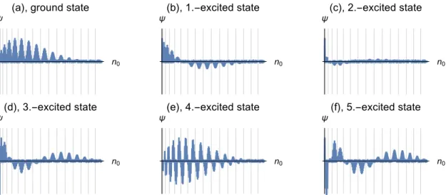
n0,−, (20)

which corresponds to the total number of particles in the zero modes, we can rearrange the Fock basis into several blocks. Figure3shows the wavefunction of the ground state and the first five excited states of the system forN

=

_120,L

=

_0,αN

=

0.7. The vertical grid lines indicate the borders between the different blocks of the Fock basis which are arranged in ascending values ofn0. Within one block the states are further sorted with respect ton_imb≡n0,+−n0,−which characterizes the imbalance between the occupation of the zero modes of a Fock state.

n0

ψ

(a), ground state

n0

ψ

(b), 1.-excited state

n0

ψ

(c), 2.-excited state

n0

ψ

(d), 3.-excited state

n0

ψ

(e), 4.-excited state

n0

ψ

(f), 5.-excited state

Figure 3.The wavefunctionsψof the six energetically lowest states forαN=0.7,L=0 andN=120.

Along the horizontal axis we order the Fock basis for fixedNandLinto sectors of constant zero mode occupationn0 = _n0,++_n0,−, and within these blocks, we further order the basis according to the imbalance between the zero modesn0 =n0,+−n0,−. The further subordering, using the last two remaining degrees of freedom, is not chosen in a specific way. This representation exhibits particle in a box-type excitations in the sectors of constantn₀.

Inspection of the wavefunctions in Figure 3 indicates a further substructure: Within each n₀-subspace the wavefunction has a form corresponding to the ground (see panels Figure 3a–d and Figure3f) or excited (see Figure3e) state of a particle in a box whereas over the whole Fock space these fine structures are enveloped by an overall oscillation. Going even further, this kind of behaviour can be compared to the excitation spectrum of a molecule in the Born-Oppenheimer approximation [31]. In this picture, the behaviour within a constantn₀-subspace corresponds to a fast degree of freedom which separates the energy spectrum into different channels [32]. Within each channel, there are smaller excitations which are determined by the slow degree of freedom corresponding to the behaviour of the oscillations in the envelope.

Based on this physical motivation we now take a look at the matrix representation of the Hamiltonian (8). If we chooseN>0 and order the Fock basis in blocks of constantn0including both paritiesP

=

±1, one obtains a tridiagonal block matrix

H

=





















H0 H0,2 0

H2,0 H2 . .. . ..

0 . .. ... . .. 0

. .. ... HN−2 HN−2,N

0 HN,N−2 H_N





















, (21)

where Hn₀ is the projection of the Hamiltonian (8) into the subspace with fixedn0, while Hn₀±2,n₀

couples then0-block to its next neighbours. Due to the form of the interaction all other blocks vanish. The next step is to define transformationsUn₀ which diagonalizeHn₀ and thereby the global transformation

U

=



















 U₀ 0

0 U2 . ..

. .. ... . ..

. .. UN−2 0

0 UN





















(22)

from the Fock space into a basis that diagonalizes each projection of the Hamiltonian (8) to an n₀-subspace. This allows us to systematically select vectors solely corresponding to the ground, first or second excited states of the channels and project out all the others. This projection then neglects all possible couplings between different channels. Please note that this procedure has to be repeated for everyαNas the magnitude of the interaction alters the corresponding eigenvectors of then0-blocks.

The resulting spectrum is shown in Figure4. Neglecting the coupling of different channels is fully justified as seen from the excellent agreement between the exact and approximated spectrum.

0.2 0.4 0.6 0.8 1.0

αN 1

2 3 4 Energy

Figure 4.Spectrum based on the adiabatic approximation (22) (dots) compared to the exact spectrum (lines) atN = 70,L = 0. The approximated dots are obtained by restriction to the ground state (red), first (black) and second (green) excited state within the fast degree of freedom. Scaled units [E] = _R^¯h used.

Here, the solid blue lines show the energy levels of the full Hamiltonian (8). In comparison, the dotted lines show the excitation spectrum if the Hamiltonian is restricted to different single channels. They correspond to restrictions to the ground state (red), first (black) and second (green) excited state within the fast degree of freedom. The excellent agreement shows that this approximation provides energy levels of the original system quantitatively to very good accuracy. Furthermore, it enables us to split the spectrum into several subspectra which can be investigated independently of each other.

4. Effective Hamiltonian

The subsequent derivation is carried out for chosen particle numberNand total momentumL, such that the respective operators are replaced by these quantum numbers. To properly derive the block structure of the Hamiltonian (8), an operator ˆPn₀ can be defined that projects the Hilbert space onto its subspace with constantn₀. By definition we have

∑

N n₀=0

Pˆn₀

=

ˆ1, (23)

which can be used to rewrite the Hamiltonian as Hˆ

= ∑

n₀,n⁰₀

Pˆ_n⁰

0

HˆPˆn₀

= ∑

n₀

Hˆeff

(

n0

) + ∑

n₀,n⁰₀

Hˆcoup

(

n⁰₀,n0

)

, (24)

where the second term is the coupling Hamiltonian. The part diagonal inn0is the effective Hamiltonian Hˆ_eff

(

n0

) =

H^ˆ0

(

n0

) +

H^ˆ1

(

n0

) +

H^ˆ2

(

n0

)

, (25)

that defines the adiabatically separated channels. In this divisionH0

(

n0

)

represents the kinetic part of the Hamiltonian (8).H₂

(

n₀

)

are the parts of the interaction which contain bosonic operatorsa_k,σ, ˆa_k,σ withk∈ {±1}and commute with ˆn0. Last of all inH1

(

_n0

)

we summed up all the remaining parts of the interaction, which commute with ˆn0. ThisH_effis the starting point of all further analysis.

4.1. Redefinition of Zero Modes

The effective Hamiltonian (25) has an additional constant of motion, Fˆ≡

∑

σ=±1

ˆ

a^†_0,σaˆ0,−σ (26)

that can be easily shown to commute also with ˆN and ˆL. The redefinition of the creation and annihilation operators of the zero modes

ˆ z±≡ √¹

2

(

aˆ0,+±aˆ0,−

)

(27)

gives

σ=±1

∑

ˆ

a^†_0,σaˆ0,σ →zˆ^†₊zˆ+−zˆ^†₋zˆ−, (28) while ˆn0

=

zˆ^†₊zˆ+

+

zˆ^†₋zˆ−keeps its structure. A further definition offers a new good quantum number necessary to describe the effective system:

ˆ

c₀

=

zˆ^†₊zˆ+,

[

H^ˆ_eff

(

n₀

)

_{, ˆ}c₀

] =

_0. (29) Therefore we are able to rewrite ˆH₁

(

n₀

)

in diagonal form as

Hˆ₁

(

n₀

) =

^α

2

(

2N−n₀−2

)(

2 ˆc₀−n₀

)

, (30) where the range of this new quantum quantum numberc0∈ {0, 1, . . . ,n0}depends onn0. Please note that the operator ˆc0is deliberately choosen in a way such that the resulting eigenenergy

E1

(

n0,c0

) =

^α

2

(

2N−n0−2

)(

2c0−n0

)

(31) of ˆH1

(

n0

)

is minimal forc0

=

0.

4.2. Redefinition of Kinetic Modes

Now we focus on the remaining parts of the effective Hamiltonian (25) to show how it can be rendered diagonal by a redefinition of the creation and annihilation operators. Up to now ˆH_eff

(

n0

)

(25) consists of two parts. While the first one (E₁

(

n₀,c₀

)

) was analyzed in Section4.1, the second part looks comparatively difficult:

Hˆ0

(

n0

) +

H^ˆ2

(

n0

) = ∑

k∈{−1,1} σ∈{−,+}

σk·aˆ^†_k,σaˆk,σ

+ ∑

k=±1

−^α

4

(

3N

+

n0

+

k·L−2

)

h^ˆk, (32)

where ˆhkis defined as

hˆ_k≡aˆ^†_k,+aˆk,−

+

aˆ^†_k,−aˆ_k,+,k∈ {±1}. (33) It is quadratic in the creation and annihilation operators

ˆ

a^†_k,+aˆk,−,k∈ {±1}, (34)

suggesting to define a vector

v≡_{aˆ1,+ aˆ1,− aˆ−1,+ aˆ−1,−}^T, (35) containing all annihilation operators of the (k

=

±1)-modes, that allows us to rewrite the Hamiltonian (32) as

Hˆ0

+

H^ˆ2

=

v^†Mv, M≡ ^{A+ 0} 0 A−

!

, (36)

where

A+ ≡ ¹ −^α₄

(

K−L

)

−^α₄

(

K−L

)

−1

!

, A−≡ −1 −^α₄

(

K

+

L

)

−^α₄

(

K

+

L

)

1

!

, (37)

andK>0 depends onNandn0via

K≡3N

+

n0−2. (38)

The quadratic form (36) allows us to diagonalize the Hamiltonian (32). From the blockstructure of the matrix one can already conclude that the diagonalization will only mix those operators within the same k-mode,

ˆ p+

ˆ p−

!

≡C+ aˆ1,+

ˆ a1,−

!

, nˆ+

ˆ n−

!

≡C− aˆ−1,+

ˆ a−1,−

!

, (39)

whereC±are matrices obtained from the eigenvectors ofA±. This notation is chosen in such a way that “p” corresponds to the new operators obtained from the operators acting on “positive”k-modes and “n” from the “negative” ones. Furthermore, the “

+

”, “−” indices (not to be confused with the eigenvalues of the parity operator) of the new operators refer to the associated eigenvalues of the diagonalized matrix

C±A±C_±^T

=



 q

1

+ (

^α₄

(

K∓L

))

² 0

0 −^q1

+ (

^α₄

(

K∓L

))

²



. (40) As this redefinition is a rotation of the old operators, the sum of their occupation numbers remains unaffected,

ˆ

n1≡nˆ1,+

+

nˆ1,−

=

aˆ^†_1,+aˆ1,+

+

aˆ^†_1,−aˆ1,−

=

pˆ^†₊pˆ+

+

pˆ^†−pˆ−, (41) and the same holds true for the negative k-modes

ˆ

n−1≡nˆ−1,+

+

nˆ−1,−

=

aˆ^†_−1,+aˆ−1,+

+

aˆ^†_−1,−aˆ−1,−

=

nˆ^†₊nˆ+

+

nˆ^†₋nˆ−. (42) Finally, in view of the transformation from Section4.1, we are able to fully diagonalize the effective Hamiltonian (25)

Hˆ_eff

(

n0

) =

^α

2

(

2N−n0−1

)(

2 ˆc0−n0

)+

r 1

+

^α

4

(

K−L

)

²·

(

pˆ^†₊pˆ+−pˆ^†₋pˆ−

) +

r 1

+

^α

4

(

K

+

L

)

²·

(

nˆ^†₊nˆ+−nˆ^†₋nˆ−

)

.

(43)

This can be made explicit using the eigenbasis of the operators ˆ

c+≡ pˆ^†₊pˆ+, cˆ− ≡nˆ^†₊nˆ+, (44) that commute with ˆH_eff

(

n₀

)

. Using

L

=

n₁−n−1, N−n₀

=

n₁

+

n−1, (45) one gets the explicit expression

E_eff

(

n₀,c₀,c+,c−

) =

^α

2

(

2N−n₀−1

)(

2c₀−n₀

) +

r

1

+

^α

4

(

K−L

)

²·

2c+− ^N−n0

+

L 2

+

r

1

+

^α

4

(

K

+

L

)

²·

2c−− ^N−n₀−L 2

(46)

for the eigenenergies. Please note that the range of the new quantum numbers c± ∈

0, 1, . . . ,N−n0±L 2

(47) is defined byN,Landn0, while in the case ofL

=

0, (46) simplifies to

E_eff

(

n₀,c₀,c+,c−

) =

^α

2

(

2N−n₀−1

)(

2c₀−n₀

) +

r

1

+

^α 4K2

·

(

2

(

c+

+

c−

)

−

(

N−n₀

))

. (48) Each combination of quantum numbers

(

c0,c+,c−

)

then defines a different channel within the effective Hamiltonian (43). In a last step, we assume that interactions between different channels can be neglected as motivated in Section 3. Within an

(

c0,c+,c−

)

-channel this leaves only one possible combination

ˆ

p^†−nˆ^†−zˆ−zˆ− (49) and its Hermitian conjugate, leading to an approximated single-channel Hamiltonian

Hˆapprox

(

c₀,c+,c−

) =

E_eff

(

nˆ₀,c₀,c+,c−

)

− ^α 2

1

+

√ ^aˆ 1

+

aˆ²

ˆ

p^†₋nˆ^†₋zˆ−zˆ−

+

h.c.

with ˆa≡ ^α

4

(

3N

+

nˆ0−2

)

(50)

for the channel labeled by

(

c0,c+,c−

)

.

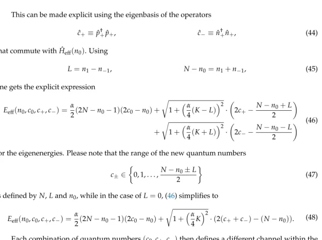
Figure 5 presents the decoupled energy spectrum of this system resulting from the Hamiltonian (50). The contribution ofc+andc−to the approximate energyE_eff

(

n0,c0,c+,c−

)

depends only on their sum c+

+

c− for the case L

=

0, and therefore c− was chosen to be always zero.

The resulting spectrum is plotted (marked by dots) against the one (solid lines) from the complete Hamiltonian (8). While the higher excitations show small deviations, the results are essentially the same as without the approximation. In particular, as the main interest is in the lowest channel which corresponds to the black dots, the new quantum numbers give rise to the ability to split the spectrum into several combinations of{c0,c+,c−}. Further investigations will be focused on the ground state and the lowest excitations which means that these quantum numbers are always chosen to be zero.

0.2 0.4 0.6 0.8 1.0 αN 1

2 3 4 Energy

c₀ c₊ c_- 0 0 0 1 0 0 0 1 0 1 1 0 2 0 0 0 2 0

Figure 5. The exact energy spectrum (solid) evaluated for N = 70, L = 0. Above it is plotted the decoupled energy spectrum (dots), obtained by numerical diagonalization of (50), with the corresponding effective quantum numbers. In choice of the parameters and approximations this is equivalent to Figure4, but after the previous derivation the division into several channels is now structured by the effective quantum numbers. Scaled units[E] =_R^¯h used.

5. Classical Analysis

In the following, we will analyse the critical properties of our effective model (50) by means of a semiclassical analysis. Starting with the diagonal part (43)

Hˆ_eff

(

n0

) =

^α

2

(

2N−n0−1

)(

zˆ^†₊zˆ+−zˆ^†₋zˆ−

) +

r 1

+

^α

4

(

3N

+

n₀−2

)

²·

(

pˆ^†₊pˆ+−pˆ^†₋pˆ−

+

nˆ^†₊nˆ+−nˆ^†₋nˆ−

)

_,

(51)

we substitute the creation/annhihlation operators by classical phase space variables

fˆ_σ →^pn_f,σ·e^iφf,σ, f ∈ {z,p,n}, σ∈ {+,−}, (52) and neglect all terms of orderO

(

N⁰

)

in the limit ofN→∞, to obtain

Eeff,cl

=

^α

2

(

2N−n0

)(

nz,+−nz,−

) +

cosh

(

γ

)(

np,+−np,−

+

nn,+−nn,−

)

, sinh

(

γ

(

_α,N,n₀

))

≡ ^α

4

(

3N

+

n₀

)

(53)

where “cl” refers to the classical (mean field) limit. Since the coupling between different channels can be neglected, as shown in Sections3and4, the classical form of the remaining interaction then gives

H_coup,cl

(

n0

) =

^α

2

(

1

+

tanh

(

γ

))

nz,−√

np,−nn,−·cos

(

2φz,−−φp,−−φn,−

)

. (54) To get an easily solvable form we reduce the Hamiltonian (51) to its channel of minimal energy by setting

nz,+

=

np,+

=

nn,+

=

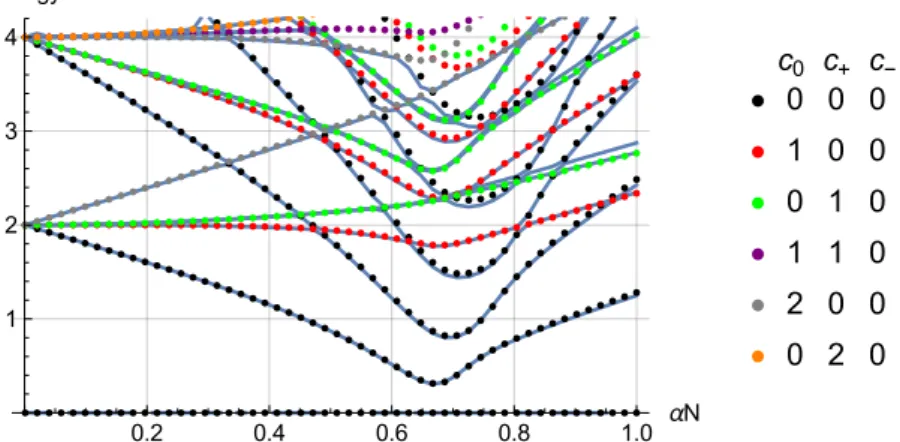
0, (55)

while we reexpress{nz,−,np,−,nn,−}in terms ofN,Landn0through the point transformation

n0

=

nz,−, np,−

=

nn,−

=

^N−n0

2 , θ

=

φz,−−¹

2

(

φp,−

+

φn,−

)

, θ_N

=

¹

2

(

φp,−

+

φn,−

)

, θ_L

=

¹

2

(

φp,−−φn,−

)

.

(56)

This finally leads to a one-dimensional description with only two (conjugate) phase-space coordinates n0andθ,

E_cl

(

α,φ,z

) =

−cosh

(

γ

)(

N−n0

)

−^α

2n0

((

2N−n0

) + (

N−n0

) (

1

+

tanh

(

γ

))

cos

(

2θ

))

. (57) To extract the physical properties of this mean field Hamiltonian (57), valid for limN→∞, we define scaled variables

e_cl

=

^Ecl

N, z

=

ⁿ⁰

N ∈

[

0, 1

]

, α¯

=

αN, sinh

(

γ

) =

sinh

(

γ

(

α,¯ z

)) =

^α¯

4

(

3

+

z

)

(58) to get the energy per particle as

e_cl

(

α,¯ θ,z

) =

−cosh

(

γ

(

α,¯ z

))(

1−z

)

−^α¯

2z

((

2−z

) + (

1−z

) (

1

+

tanh

(

γ

(

α,¯ z

)))

cos

(

2θ

))

. (59) We are now ready to proceed with the study of the classical phase space. Obviously, it isπ-periodic inθsuch that the analysis can be restricted toθ∈

[−

^π₂,^π₂

]

.

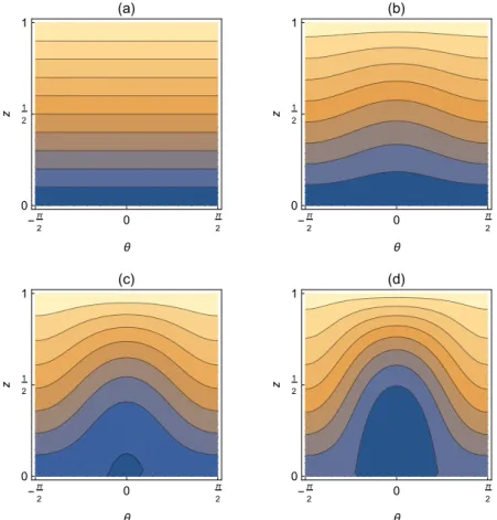
Figure6shows contour plots of the energye_clfor different values of the coupling ¯α. As clearly seen, there is a qualitative change within the phase space, when the scaled interaction is increased from ¯α

=

0 and ¯α

=

1. While in the non-interacting case, the phase space allows only rotations (Using the analogy to the mathematical pendulum), the phase space is divided into two qualitatively different regions at ¯α

=

1. The regime of the lowest energies consists of vibrations/librations, separated from the rotating orbits by a separatrix. This separatrix is created atz

=

φ

=

0 at a critical interaction αcrit. Furthermore, for weak interaction (0≤α¯ ≤α¯crit) the energy minimum is located atz

=

0 and degenerate inθ. In contrast, at a stronger interaction (¯α_crit<α), the energy minimum consists of only¯ one discrete pointz>0,θ

=

0.

According to its definition,zrepresents the ratio of particles within the zero modesn0,+andn0,−

with respect to the whole particle numberN. This yields the interpretation that, for an interaction greater than ¯α_crit, the occupation of the zero modes within the ground state changes from a microscopic occupation near zero to a macroscopic one at a finite value and therefore indicates thatzcan be taken as an order parameter characterizing a type of quantum phase transition. Since in this model there is no physical ground state, the abrupt changes that characterize quantum phase transition happen now around an effective, pseudo-ground state, and properly speaking we should refer to this as a pseudo-quantum phase transition. In the spirit of not overcharging with new terminology the manuscript, however, we used and continue using the term quantum phase transition along the text.

This is in complete analogy with the spin-one Bose gas without pseudospin and quadratic Zeeman shift [33] and the truncated versions of the attractive one-dimensional Bose gas [21].

-^π

2

0 ^π

2

0

1 2

1

θ

z

(a)

-^π

2

0 ^π

2

0

1 2

1

θ

z

(b)

-^π

2

0 ^π

2

0

1 2

1

θ

z

(c)

-^π

2

0 ^π

2

0

1 2

1

θ

z

(d)

Figure 6.Phase diagram ofe_clfor ¯α=0 (a), ¹₃(b), ²₃ (c), 1 (d). z= ⁿ_N⁰ is the normalized zero mode occupation andθ the conjugate phase.. The color scaling describes the value of the energy. Blue represents the minimum and light orange the maximum.

6. Analytic Analysis of the Quantum Phase Transition

Armed with a clear signature of a phase transition in the change of morphology of the classical (mean field) limit produced by the appearance of the separatrix, we will now study the different aspects of this critical behaviour. As discussed before in Section5, the energy minimum is always located at θ

=

0 for ¯α>α¯_critand is degenerate inθfor ¯α≤α¯_crit. Therefore, this variable can be eliminated in the following discussion by settingθ

=

0. The resulting energy dependencee_cl

(

α,¯ θ

=

0,z

)

onzfor several

¯

αis shown in Figure7.

-¹

2 0 ¹

2 1

-1.0 -0.8 -0.6 -0.4 -0.2

e_{0, cl}

(a)

-¹

2 0 ¹

2 1

-1.0 -0.8 -0.6 -0.4

e_{0, cl}

(b)

-¹

2 0 ¹

2 1

-1.2 -1.0 -0.8 -0.6 -0.4

e_{0, cl}

(c)

Figure 7.e_cl(α,¯ θ=0,z)forαN= 0.4 (a), 0.6 (b), 0.8 (c).

The range ofzwas deliberately chosen as{−¹₂, 1}, despite the fact that negativezare unphysical according to its definition, to illustrate the behaviour of the local minimum depending on the interaction strength ¯α. For ¯α≤α¯_critthis minimum would be atz^∗ <0. As this is not part of the allowed phase

space, the minimum will simply be located atz^∗

=

0. If the interaction strength is increased,z^∗ increases too until it reachesz^∗

=

0. This is exactly the point where the quantum phase transition can be expected. To find the critical value, one cane use that the derivative of the energyeclwith respect to zshould vanish when evaluated atz

=

0 and ¯α

=

α¯_crit

∂ecl

(

α¯_crit,θ

=

0,z

)

∂z

_z=0

=

−^3¯αcrit

2

+

_q ⁴

16

+

9¯α²_crit

=

0, (60)

which provides the critical parameter as

¯ α_crit

=

²

3 q

2

(

√

2−1

)

≈0.607. (61)

To further prove this critical behaviour, Figure8shows the functional dependence of the second derivative of energy minimum with respect to ¯α,

∂²e_cl

(

α,¯ θ

=

0,zmin

)

∂²α¯ , with e_cl

(

α,¯ θ

=

0,zmin

)

≡e_cl,min

(

α¯

)

. (62) The plot consists of four curves and a dashed line indicating the exactN → ∞values of the discontinuity. All the curves are based on values of the groundstate energy for discrete sets of points of ¯α, with the second derivative evaluated numerically. The blue dots were calculated using the energy dependence given by the classical Hamiltonian (59), whose minimal energy was numerically determined within the phase space for different values of ¯α. They are compared to the quantum mechanical results for the ground state at various particle numbersNgiven by the lowest eigenvalue of the matrix representation of (50) renormalized by _N¹.

The analytical resulte⁰⁰_0,<

(

α¯

)

, is obtained through a simple derivative of the classical energy with respect tozat the critical point

e⁰⁰_0,<

(

α¯_crit

) =

^∂

2e_cl

(

α¯_crit,θ

=

0,z

)

∂²z

_z=0

=

− ⁹

4√ 2

1

+

√

23/2 ≈ −0.424. (63) Extracting the second value right behind the critical threshold is a bit harder, as the change of the z-position depending on ¯αhas to be taken into account. To this end a leading-order expansion inz is necessary

z

(

α¯

) =

z

(

α¯crit

) +

^∂z

∂¯α _¯α=¯

αcrit

(

α¯−α¯crit

) +

O

((

α¯−α¯crit

)

²

)

≈z⁰

(

α¯crit

)(

α¯−α¯crit

)

, (64) where we usedz

(

α¯crit

) =

0.

Now problem is reduced to calculating the derivative ofzwith respect to ¯αat the critical point.

For this purpose we define the function

g

(

α,¯ z

) =

^∂e

(

α,¯ θ

=

0,z

)

∂z . (65)

The zero of this function for a chosen ¯αgives thez-position of the energy minimum and therefore its derivative is

∂z

∂α¯ _{α=¯ ¯}

αcrit

=

− ∂g

∂z −1

α¯crit,z(¯αcrit)=0

∂g

∂α¯

α¯crit,z(¯αcrit)=0

. (66)

The last step is to insert ¯αinto

e_cl

(

α,¯ θ

=

0,z

)

→e_cl

(

α,¯ θ

=

0,z

(

α¯

) =

z⁰

(

α¯crit

)(

α¯−α¯crit

))

(67) and to calculate the second derivative

∂²e_cl

(

α,¯ θ

=

0,z

(

α¯

))

∂²α¯

=

− ⁹ 1156

s373469

√2 −³²⁵⁵⁹¹

2 ≈ −2.478. (68)

Clearly, the dependence of the ground state energy is seen to be discontinuous at ¯α

=

α¯_critwith

¯

α_critdetermined in the previous section. With the last results we even obtained an analytic expression to quantify the magnitude of the discontinuity

e⁰⁰_0,<−e_0,>⁰⁰

=

⁸¹ 289

q 569√

2−751≈2.05, (69)

in excellent agreement with the numerical result shown in Figure8.

x x x x x x x x x x x x x x x x x x x x x x xx x xx xx xx

x x

x x

x x

x x xx

x

xxxx xx xx x x x x x x x x x x x x x x x x x x x x x x x x x x x

x x

x

x x

xx xx xx x xx x xx x xx x xx x x x x x x x x x x x x x x x x x x x x x x x x x x x x

x

xx xx x xx x xx x xx x xx x xx x x

0.56 0.58 0.60 0.62 0.64

α

-2.5 -2.0 -1.5 -1.0 -0.5 E₀''(αN) /N

x qm: N=500

x qm: N=5 000

x qm: N=50 000 classical

e^''_0,<

e^''_0,>

Figure 8.Second derivative of the ground state energy with respect to ¯α. Scaled units[E] = ^h_R^¯ used.

7. Further Characterization of the Critical Behaviour

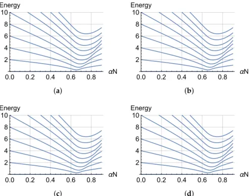
In this last section, we will further characterize the finite-size effects in the quantum phase transition by means of the way the critical parameters approach their sharp values in the mean field limitN→∞. Our choice of the appropriate observables comes from the behaviour of the spectrum when we approach the critical region. As seen in Figure9, and in accordance with what happens in the attractive Lieb-Liniger model [21], one observes a strong accumulation of excited states around criticality, a phenomenon that can be related to an excited-state quantum phase transition [34,35].

The structure of the spectrum in Figure9and the dependence shown in Figure10suggests that the approach to criticality is well captured by two parameters, namely the minimal gap and interaction value describing its position,

N→lim∞∆Egap

=

0, lim

N→∞

(

α¯gap−α¯_crit

) =

0, (70) in the form of a power laws

∆Egap∝N^−β, ∆α¯_gap≡α¯_gap−α¯_crit∝N^−γ, (71) whereβ,γ> 0, will be referred to as dynamical exponents [26].

0.0 0.2 0.4 0.6 0.8 αN 2

4 6 8 10 Energy

0.0 0.2 0.4 0.6 0.8 αN 2

4 6 8 10 Energy

0.0 0.2 0.4 0.6 0.8 αN 2

4 6 8 10 Energy

0.0 0.2 0.4 0.6 0.8 αN 2

4 6 8 10 Energy (a)

0.0 0.2 0.4 0.6 0.8 αN 2

4 6 8 10 Energy

0.0 0.2 0.4 0.6 0.8 αN 2

4 6 8 10 Energy

0.0 0.2 0.4 0.6 0.8 αN 2

4 6 8 10 Energy

0.0 0.2 0.4 0.6 0.8 αN 2

4 6 8 10 Energy (b)

0.0 0.2 0.4 0.6 0.8 αN 2

4 6 8 10 Energy

0.0 0.2 0.4 0.6 0.8 αN 2

4 6 8 10 Energy

0.0 0.2 0.4 0.6 0.8 αN 2

4 6 8 10 Energy

0.0 0.2 0.4 0.6 0.8 αN 2

4 6 8 10 Energy (c)

0.0 0.2 0.4 0.6 0.8 αN 2

4 6 8 10 Energy

0.0 0.2 0.4 0.6 0.8 αN 2

4 6 8 10 Energy

0.0 0.2 0.4 0.6 0.8 αN 2

4 6 8 10 Energy

0.0 0.2 0.4 0.6 0.8 αN 2

4 6 8 10 Energy (d)

Figure 9.Illustration of convergence of the ten lowest energylevels in the first channel towards the critical point forN=100 (a), 500 (b), 1000 (c), 5000 (d). Scaled units[E] = _R^¯h used.













ΔE

_gap

α

_gap

α

_crit

0.607 0.608 0.609 0.610

α 0.02

0.04 0.06 0.08 0.10

Energy

Figure 10. Energy gap∆Egap for N = 20 000 with ¯α_min = 0.606 and ¯αmax = 0.610. Scaled units [E] = _R^h¯ used.

To this end the gap is numerically calculated in a small region between specifically chosen

¯

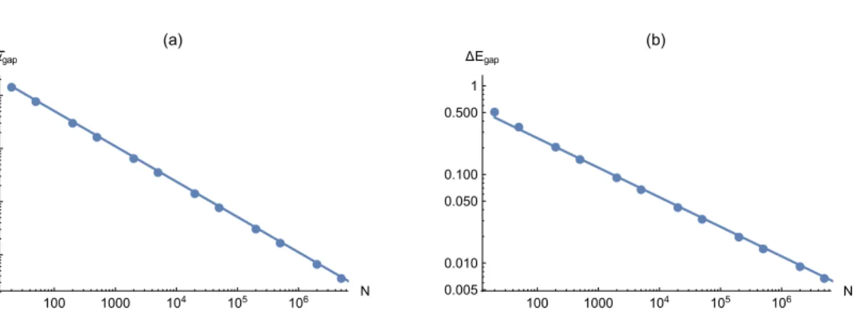
α_min, ¯αmaxfor a given particle numberN. Afterwards, an interpolation function is calculated within this region and the minimum of it is numerically determined. This procedure is repeated for several N. Because of its special behaviour at the phase transition, the necessary numerical effort can be reduced drastically [36]. By means of this numerical approach, we are able to present results with particle numbers between twenty and five million. The results are shown in Figure11using a double logarithmic scale.

 

 

 

 

 

 

100 1000 10⁴ 10⁵ 10⁶ N

10^-4 0.001 0.010 0.100

Δ α_gap

(a)

 

 

 

 

 

 

100 1000 10⁴ 10⁵ 10⁶ N

0.005 0.010 0.050 0.100 0.500 1 ΔEgap

(b)

Figure 11. Asymptotic behaviour of the gap in interaction ¯α(a) and energy (b) depending on the particle numberNin a double logarithmic plot with linear fits.

To extract the power law the particle numbers withN≥20,000 are fitted linearly. Smaller particle numbers are taken out of the fit because this power-law is found to be valid only for large particle numbers. The obtained relations are

∆α¯_gap∝N^−0.3336, ∆Egap∝N^−0.6651, (72) where the powers seem to coincide with the values−¹₃and−²₃within small tolerance.

These scalings rule how the mean-field limitN → _∞is approached by two purely quantum observables, as by their very definition the minimal gap and corresponding critical interaction require quantization. An analytical approach that allows for a physical picture and the prediction of such scaling exponents lies therefore beyond the realm of the mean-field approach. A proper semiclassical analysis, able to study such effects by quantizing the mean-field phase space, was successfully applied for the non-relativistic, spinless case in [21,28], where the dynamical exponents were found to be exactly given by ¹₃and²₃. We expect that an extension of the semiclassical quantization of [21,28] in the present relativistic case is feasible given the close similarities in the effective phase space, and the study of the corresponding scaling laws is work in progress.

8. Summary and Conclusions

In this article, we explored a (pseudo) relativistic extension of the attractive Lieb-Liniger model, by considering both particles with linear dispersion and spin degree of freedom. Our objective was to check the existence of a relativistic analogue of the well-known quantum phase transition [26]

displayed by the original non-relativistic model, where the attractive potential drives a transition of the ground state from a homogeneous state into an inhomogeneous one due to the critical appearance of a bright soliton, as thoroughly study by means of semiclassical methods in [21].

As a main result, we find numerically and explain analytically that the relativistic extension indeed shows clear signatures of critical behaviour and a quantum phase transition where the macroscopic occupation of the side modes (|k|

=

1), characterized by the vanishing order parameter given by the occupation of the homogeneous zero modes, is destroyed by quantum fluctuations giving rise to the macroscopic occupation of the zero modes, indicating a sudden broadening of the particle distribution and an increase in the interaction energy.

Given the fact that the existence of the phase transition in the non-relativistic case is essentially due to the quantum integrability of the model, the fact that the same effect can be seen in the present non-integrable system points towards universal aspects of this transition.

To get an analytical understanding of this transition and its connection to the integrability of the non-relativistic case, we followed a combined approach. First, extensive numerical simulations show an adiabatic separation that mimics integrability in the low-energy region. Second, a classical analysis based on this approximate separability of the model allows for understanding the critical behaviour

as a consequence of the appearance of separatrix motion in the mean field limit. This combination enabled us to provide analytical results for the location and characteristics of the quantum phase transition in excellent agreement with exact diagonalization results.

Our work follows the idea of a universal connection between the characteristics of separatrix dynamics in the mean field limit and the parameters describing ground and excited state quantum phase transitions of the quantum system, a subject of particular interest in the field of many-body semiclassics.

Author Contributions:B.G. and K.R. devised the project, M.N. and B.G. were the main contributor to the work and M.N. performed the numerical simulations. J.-D.U. devised the manuscript and all the figures were produced by M.N. All authors have read and agreed to the published version of the manuscript.

Funding:B.G acknowledges financial support from the Deutsche Forschungsgemeinschaft (DFG) throgh Project No. Ri681/14-1.

Acknowledgments:All authors acknowledge discussions with Quirin Hummel. We also acknowledge a very careful reading of the manuscript by an anonymous referee, whose suggestions helped with both content and form of the paper.

Conflicts of Interest:The authors declare no conflict of interest.

References

1. Gutzwiller, M. Chaos in Classical and Quantum Mechanics (Interdisciplinary Applied Mathematics); Springer:

New York, NY, USA, 1991.

2. Haake, F.Quantum Signatures of Chaos; Springer: Berlin/Heidelberger, Germany, 2010.

3. Grempel, D.R.; Prange, R.E.; Fishman, S. Quantum dynamics of a nonintegrable system.Phys. Rev. A1984, 29, 1639. [CrossRef]

4. Georgeot, B.; Prange, R. Exact and Quasiclassical Fredholm Solutions of Quantum Billiards. Phys. Rev. Lett.

1995,74, 2851–2854. [CrossRef] [PubMed]

5. Altman, E. Many-body localization and quantum thermalization. Nat. Phys.2018,14, 979–983. [CrossRef]

6. Swingle, B. Unscrambling the physics of out-of-time-order correlators. Nat. Phys. 2018,14, 988–990.

[CrossRef]

7. Srednicki, M. Chaos and quantum thermalization. Phys. Rev. E1994,50, 888–901. [CrossRef] [PubMed]

8. Rigol, M.; Dunjko, V.; Olshanii, M. Thermalization and its mechanism for generic isolated quantum systems.

Nature2008,452, 854–858. [CrossRef] [PubMed]

9. Eisert, J.; Friesdorf, M.; Gogolin, C. Quantum many-body systems out of equilibrium. Nat. Phys.2014, 11, 124–130. [CrossRef]

10. Larkin, A.I.; Ovchinnikov, Y.N. Quasiclassical Method in the Theory of Superconductivity. Sov. J. Exp.

Theor. Phys.1969,28, 1200.

11. Maldacena, J.M.; Shenker, S.H.; Stanford, D. A bound on chaos. J. High Energy Phys. 2016,2016, 1–17.

[CrossRef]

12. Maldacena, J.; Stanford, D. Remarks on the Sachdev-Ye-Kitaev model. Phys. Rev. D2016,94, 106002.

[CrossRef]

13. Rammensee, J.; Urbina, J.D.; Richter, K. Many-Body Quantum Interference and the Saturation of Out-of-Time-Order Correlators. Phys. Rev. Lett.2018,121, 124101. [CrossRef] [PubMed]

14. Emary, C.; Brandes, T. Chaos and the quantum phase transition in the Dicke model. Phys. Rev. E2003, 67, 066203. [CrossRef] [PubMed]

15. Bastidas, V.M.; Pérez-Fernández, P.; Vogl, M.; Brandes, T. Quantum Criticality and Dynamical Instability in the Kicked-Top Model. Phys. Rev. Lett.2014,112, 140408. [CrossRef]

16. Bastarrachea-Magnani, M.A.; López-del-Carpio, B.; Chávez-Carlos, J.; Lerma-Hernández, S.; Hirsch, J.G.

Regularity and chaos in cavity QED.Phys. Scr.2017,92, 054003. [CrossRef]

17. Engl, T.; Dujardin, J.; Argüelles, A.; Schlagheck, P.; Richter, K.; Urbina, J.D. Coherent Backscattering in Fock Space: A Signature of Quantum Many-Body Interference in Interacting Bosonic Systems. Phys. Rev. Lett.

2014,112, 140403. [CrossRef] [PubMed]

18. Engl, T.; Urbina, J.D.; Richter, K. Periodic mean-field solutions and the spectra of discrete bosonic fields:

Trace formula for Bose-Hubbard models.Phys. Rev. E2015,92, 062907. [CrossRef] [PubMed]